HAL Id: hal-00298375
https://hal.archives-ouvertes.fr/hal-00298375
Submitted on 17 May 2006HAL is a multi-disciplinary open access
archive for the deposit and dissemination of sci-entific research documents, whether they are pub-lished or not. The documents may come from teaching and research institutions in France or abroad, or from public or private research centers.
L’archive ouverte pluridisciplinaire HAL, est destinée au dépôt et à la diffusion de documents scientifiques de niveau recherche, publiés ou non, émanant des établissements d’enseignement et de recherche français ou étrangers, des laboratoires publics ou privés.
Interannual variations of water mass properties and
volumes in the Southern Ocean
M. Tomczak, S. Liefrink
To cite this version:
M. Tomczak, S. Liefrink. Interannual variations of water mass properties and volumes in the Southern Ocean. Ocean Science Discussions, European Geosciences Union, 2006, 3 (3), pp.199-219. �hal-00298375�
OSD
3, 199–219, 2006Variation of Southern Ocean water mass
volumes M. Tomczak and S. Liefrink Title Page Abstract Introduction Conclusions References Tables Figures J I J I Back Close Full Screen / Esc
Printer-friendly Version Interactive Discussion Ocean Sci. Discuss., 3, 199–219, 2006
www.ocean-sci-discuss.net/3/199/2006/ © Author(s) 2006. This work is licensed under a Creative Commons License.
Ocean Science Discussions
Papers published in Ocean Science Discussions are under open-access review for the journal Ocean Science
Interannual variations of water mass
properties and volumes in the Southern
Ocean
M. Tomczak and S. Liefrink
School of Chemistry, Physics and Earth Sciences, the Flinders University of South Australia, GPO Box 2100, Adelaide SA 5001, Australia
Received: 29 March 2006 – Accepted: 8 April 2006 – Published: 17 May 2006 Correspondence to: M. Tomczak ([email protected])
OSD
3, 199–219, 2006Variation of Southern Ocean water mass
volumes M. Tomczak and S. Liefrink Title Page Abstract Introduction Conclusions References Tables Figures J I J I Back Close Full Screen / Esc
Printer-friendly Version Interactive Discussion
Abstract
Time-resolving optimum multi-parameter (TROMP) analysis is used to study interan-nual variability of water mass properties in the Southern Ocean in a section between Antarctica and Tasmania for the period 1991–1996. Water mass properties were sta-ble during 1994–1996 but showed departures from their 1994–1996 values during 1991
5
and 1993. TROMP analysis is unable to quantify the interannual variation in detail, but it is shown that interannual variability does not invalidate the findings of a previous study that was based on the assumption of time-invariable water mass properties and suggested large interannual fluctuations in the water mass volumes south of Tasmania.
1 Introduction 10
One of the repeat sections of the World Ocean Circulation Experiment (WOCE) in the Southern Ocean was section SR03 from Tasmania to Antarctica (Rintoul and Bullister, 1999). The section was occupied five times between 1991 and 1996, offering the possibility to study variations in water mass volumes and properties on interannual scales.
15
In a previous study (Tomczak and Liefrink, 2005) evidence was presented for a de-crease in the volume of Antarctic Bottom Water (AABW), accompanied by an inde-crease in the volume of Lower Circumpolar Deep Water (LCDW), in the SR03 section. This result was derived through Optimum Multiparameter (OMP) analysis, which analyses water mass contributions on the assumption that the water properties in the
forma-20
tion regions of the water masses do not change over time (see for example Poole and Tomczak, 1999, for a description of the method). This paper addresses the question to what degree this assumption might have precluded a realistic analysis and led to erroneous results.
OSD
3, 199–219, 2006Variation of Southern Ocean water mass
volumes M. Tomczak and S. Liefrink Title Page Abstract Introduction Conclusions References Tables Figures J I J I Back Close Full Screen / Esc
Printer-friendly Version Interactive Discussion
2 Data and methods
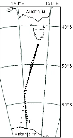
WOCE repeat section SR03 extended across one of the constriction points of the Antarctic Circumpolar Current (ACC) between 130◦E and 150◦E (Fig. 1). Following the WOCE protocol, CTD and Niskin bottle stations were taken approximately every 30 nautical miles, and more frequently over rapidly varying topography or in the vicinity
5
of the Subantarctic Front.
During 1991 weather conditions led to disruption of the section during the outbound voyage to Antarctica and completion of the section during the return voyage. The two partial data sets were combined into a single section for this study, which therefore contains five complete transects for the years 1991–1996. Table 1 gives the dates of
10
individual transects. The WOCE data provided potential temperature, salinity, oxygen, phosphate, nitrate and silicate as parameters for water mass analysis.
The previous analysis used data interpolated vertically onto a 50-m grid that covered the depth range 50–4250 m. The surveyed area was restricted to a common latitude range between 44◦42.20S and 64◦53.30S and a common bathymetry for all years. Water
15
mass volumes were determined by integration over the relative contributions of each water mass.
In contrast to the earlier study, which determined the relative contributions through OMP analysis, a further development of the method called Time-Resolving Optimum Multiparameter (TROMP) analysis is used here to determine interannual variations in
20
water mass volumes as well as source water properties.
TROMP analysis was introduced in a study of time variability in water masses found at the Bermuda Atlantic Time-series Study (BATS) in the Sargasso Sea, one of the longest oceanographic time series available today (Henry-Edwards and Tom-czak, 2005b). A detailed description of the method is given in Henry-Edwards and
OSD
3, 199–219, 2006Variation of Southern Ocean water mass
volumes M. Tomczak and S. Liefrink Title Page Abstract Introduction Conclusions References Tables Figures J I J I Back Close Full Screen / Esc
Printer-friendly Version Interactive Discussion Tomczak (2005a). Briefly, the linear system of water mass mixing equations
T1x1+ T2x2+ T3x3+ T4x4 = Tobs+ RT S1x1+ S2x2+ S3x3+ S4x4 = Sobs+ RS O1x1+ O2x2+ O3x3+ O4x4− αrO = Oobs+ RO N1x1+ N2x2+ N3x3+ N4x4+ αrN = Nobs+ RN P1x1+ P2x2+ P3x3+ P4x4+ αrP = Pobs+ RP Si1x1+ Si2x2+ Si3x3+ Si4x4+ αrSi = Siobs+ RSi x1+ x2+ x3+ x4 = 1 + RΣ
where the xi are the relative contributions from each source water type (SWT) in the observed property distribution, R are the residuals, and the last line is the mass con-straint function to ensure that the sum of water type contributions adds up to 100%,
5
is minimized by varying the xi and the SWTs (Ti, Si, Oi, Ni, Pi and Sii). This results in a highly underdetermined nonlinear problem and requires the careful evaluation of constraints to guide the method to a physically sensible and oceanographically realistic solution.
In the minimisation, a weighting function W is added and the equation is re-arranged
10
to take the form:
R= W × (Ax − b)
where R is the vector of residuals, A the matrix of SWTs, x the vector of relative contri-butions and b the vector of measured water properties. A non-negativity constraint is introduced to avoid negative water mass contributions.
15
TROMP analysis turns the overdetermined linear system of OMP equations into a highly underdetermined nonlinear problem with an infinite range of solutions. Finding the correct constraints to guide the analysis to the oceanographically most acceptable solution is the major task of TROMP analysis. Henry-Edwards and Tomczak (2005a) recommended a sequence of steps to define the most appropriate constraints and
20
arrive at an acceptable solution:
OSD
3, 199–219, 2006Variation of Southern Ocean water mass
volumes M. Tomczak and S. Liefrink Title Page Abstract Introduction Conclusions References Tables Figures J I J I Back Close Full Screen / Esc
Printer-friendly Version Interactive Discussion Step 1: A series of TROMP analyses is performed in which individual source water
properties are varied across all source water types simultaneously, whilst keeping all other source water properties constant.
Step 2: The resulting error fields and analysis output are evaluated, to identify source water properties that may be varying during the analysis period.
5
Step 3: A targeted TROMP analysis is performed in which only the source water prop-erties and source water types identified as changing are allowed to vary.
The minimization procedure employs an iterative process in two alternating modes; the first defines initial values, while the second performs the actual minimisation. Mode 1 uses SWT values from the previous iteration stage to determine the relative
con-10
tributions of each water mass at the current iteration stage through OMP analysis. Mode 2 takes the relative contributions determined from mode 1 and the SWT val-ues from the previous iteration stage as starting valval-ues for a constrained minimisation. While Henry-Edwards and Tomczak (2005a) used TROMP analysis to follow monthly changes of SWTs through a decade, in the present application the method is used for
15
each individual year of the observation period separately, with the aim to improve the initial SWT definitions by allowing them to differ from year to year.
3 Water masses
Eight water masses determine the hydrographic characteristics of the WOCE SR03 Repeat Section. Tomczak and Liefrink (2005) reviewed their origin and properties in
20
detail, so only a brief summary is given here. Summer Surface Water (SSW) is a highly variable layer found above a seasonal halocline characterised by low salinity. Antarctic Winter Water (AAWW) is a temperature minimum layer found below the SSW. Western South Pacific Central Water (WSPCW) forms through subduction at the Subtropical Convergence of the region. Subantarctic Mode Water (SAMW) is formed by deep
OSD
3, 199–219, 2006Variation of Southern Ocean water mass
volumes M. Tomczak and S. Liefrink Title Page Abstract Introduction Conclusions References Tables Figures J I J I Back Close Full Screen / Esc
Printer-friendly Version Interactive Discussion convection in late winter on the equatorward side of the Antarctic Circumpolar
Cur-rent (ACC) in the Southern Ocean and in the south eastern Indian Ocean. Antarctic Intermediate Water (AAIW) is identified by a prominent salinity minimum.
Circumpolar Deep Water (CDW) is the product of North Atlantic Deep Water being modified through mixing with deep waters from the Indian and Pacific Oceans during
5
its eastward passage with the ACC. The contributions from different sources can be traced to some extent, and several investigators distinguish Upper Circumpolar Deep Water (UCDW), which is characterized by an oxygen minimum and nutrient maxima, and Lower Circumpolar Deep Water (LCDW), characterized by its high NADW salinity. Antarctic Bottom Water (AABW) is formed by deep convection at the Antarctic
conti-10
nent, particularly in the Weddell Sea, the Ross Sea and Ad ´elie Land. The three regions produce AABW of slightly different characteristics. Two types of Antarctic Bottom Wa-ter, Ad ´elie Land Bottom Water (ADLBW) and Weddell Sea Bottom Water (WSBW), are found in the region under investigation and included in the present study.
The study concentrates on the depth range 1500–4500 m, where Tomczak and
15
Liefrink (2005) found the largest interannual changes of water mass volumes. Wa-ter mass properties are taken from the analysis of Tomczak and Liefrink (2005), who also provided the parameter weights for the current analysis. Four of the eight water masses (SSW, WW, WSPCW and AAIW) are not found at the depths of interest for this study and are therefore excluded from further consideration. Table 2 gives the water
20
type definitions for all water masses considered and the parameter weights used.
4 Results
Since the source water types used in the analysis were derived from the data collected during SR03, any departures of the actual SWTs from the values listed in Table 2 can be expected to be quite small. Following the procedure suggested by Henry-Edwards
25
and Tomczak (2005a) we performed a first TROMP analysis in which one SWT (tem-perature, salinity, oxygen, phosphate, nitrate or silicate) was allowed to vary in all water
OSD
3, 199–219, 2006Variation of Southern Ocean water mass
volumes M. Tomczak and S. Liefrink Title Page Abstract Introduction Conclusions References Tables Figures J I J I Back Close Full Screen / Esc
Printer-friendly Version Interactive Discussion masses (UCDW, LCDW, ADLBW and AABW), while all other SWTs were kept constant.
By comparing the resulting residuals this procedure enables us to identify which SWTs showed the largest variations during the observation period. We found that varying the potential temperature resulted in the largest reduction of the residuals, followed at some distance by variations of oxygen. Varying other SWTs had little or no effect on
5
the residuals.
Having identified potential temperature and oxygen as the SWTs with the strongest variability in time, we turned to the question which water mass might have undergone the largest SWT variation in time. To answer this question for potential temperature we performed a second TROMP analysis, in which potential temperature was the only
10
SWT allowed to vary, and this in only one water mass at a time.
The result was ambiguous and did not identify any particular water mass as being associated with the most significant time variability. The core result from this second run through the TROMP analysis was the finding that during three of the five years, allowing potential temperature to vary did not change the SWT definitions. In other
15
words, the SWT definitions given in Table 2 are the best available definitions for those three years and cannot be improved by the method. This result does not come entirely as a surprise, given the fact that the SWT definitions are based on the data set itself; but it shows that the water mass properties observed in 1994, 1995 and 1996 did not depart significantly from the mean for the period 1991–1996.
20
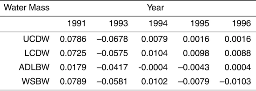
Of more interest is the fact that the two years 1991 and 1993 showed quite different behaviour. Table 3 gives the difference between potential temperature derived from this analysis run and its value given in Table 2. The differences are up to one order of magnitude larger for 1991 and 1993 than for 1994–1996. This suggest that during 1991 and 1993 water mass properties found at SR03 differed significantly from their
25
mean values for the period. It is also noteworthy that the departure from the mean values is positive during 1991 but negative during 1993.
The analysis to this point identified 1991 and 1993 as years when potential tempera-ture had undergone significant changes in one or more water mass formation regions,
OSD
3, 199–219, 2006Variation of Southern Ocean water mass
volumes M. Tomczak and S. Liefrink Title Page Abstract Introduction Conclusions References Tables Figures J I J I Back Close Full Screen / Esc
Printer-friendly Version Interactive Discussion but it did not allow identification of the water mass (or water masses) in which these
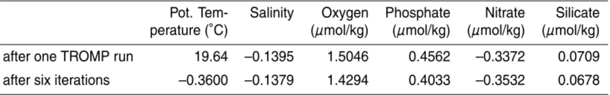
changes had occurred. Tables 4 and 5 show the situation for 1993. The very large potential temperature residual obtained from the first TROMP run is strongly reduced after six iterations (Table 4). The residuals of all other SWTs improve as well but to only minor extent. To achieve this result, TROMP analysis adjusts the potential temperature
5
of all water masses (Table 5).
The situation was quite different for 1991. Rather than reducing the SWT residuals, variation of potential temperature alone resulted in divergent behaviour. A significant reduction of the potential temperature residual could only be achieved if oxygen was allowed to vary as well. To keep the number of variables as low as possible potential
10
temperature and oxygen were not varied simultaneously but in alternate iterations. The results are displayed in Tables 6 and 7. The upper lines in the tables refer to a run in which potential temperature was set constant at every even iteration, while oxygen was set constant at every odd iteration. Likewise, the lower lines give the result when the order of iterations was reversed.
15
The results from this approach are similar to the result for 1993: a substantial re-duction in the residuals of the variable SWTs and few changes in the residuals of the other SWTs. The reduction of the potential temperature residual is not as outstanding for 1991 as for 1993, but the oxygen residual has also been decreased significantly. It can also be noted that the result shows little dependence on the order of the iteration;
20
after six iterations the residuals are very similar for both runs (Table 6), and the values obtained for the SWTs are nearly identical (Table 7).
5 Discussion
A TROMP analysis for the data obtained during WOCE repeat section SR03 con-firmed the SWT values for the Southern Ocean for the years 1994–1996 and suggested
25
changes in source water properties for the years 1991 and 1993. The analysis found an oceanographically feasible relative minimum of the residual fields for the two years.
OSD
3, 199–219, 2006Variation of Southern Ocean water mass
volumes M. Tomczak and S. Liefrink Title Page Abstract Introduction Conclusions References Tables Figures J I J I Back Close Full Screen / Esc
Printer-friendly Version Interactive Discussion The resulting variations of potential temperature amount to about 0.4◦C for UCDW and
ADLBW, 0.3◦C for LCDW, and 0.2◦C for WSBW. Whether they represent the actual oceanographic situation during 1991 and 1993 cannot be assessed without additional information and is not the aim of this paper; existing information on interannual property changes in the deep ocean is scarce and can only be used to support their plausibility.
5
Most studies of property changes in the deep ocean focus on long-term climate change and are based on comparisons of oceanographic transects performed decades apart. Bindoff and McDougall (2000) compared a section across the Indian Ocean from 1962 with a similar section from 1987 and derived basin-averaged cooling at 2000 m depth of about 0.05◦C over the 25 year period. Arbic and Owens (2001) compared
10
sections from 1925 and 1959 across the southwestern Atlantic Ocean and extrapo-lated warming of about 0.2◦C per century on isopycnals near the 2000 m depth level. Johnson and Orsi (1997) reported cooling of up to 0.07◦C on density surfaces between 1968/69 and 1990 for the South Pacific Ocean.
Santoso et al. (2006) analysed output from a coupled climate model without human
15
carbon dioxide imprint for variability of Circumpolar Water properties over ten centuries. They found that the potential temperature of UCDW and LCDW varied by about 0.2◦C over the entire period. They consider this small compared with the variations that were observed over periods of decades and explain this by pointing out the coarse grid resolution of the model, which acts like a damping mechanism, and the difference
20
between the model’s constant CO2scenario and the real world.
The apparent variations suggested by TROMP analysis (Tables 5 and 7) seem large against the reported observations and the model. It has to be kept in mind, however, that the climate model is highly damped at the interannual period range and that com-parison of oceanic sections occupied decades apart is based on the assumption that
25
interannual variability is small compared to decadal changes. Rintoul and England (2002) used the data from the SR3 repeat section for a study of SAMW variability and found a potential temperature variability of 1.3◦C. While the depth range of SAMW is above the depth range discussed in this study and property variability is likely to
in-OSD
3, 199–219, 2006Variation of Southern Ocean water mass
volumes M. Tomczak and S. Liefrink Title Page Abstract Introduction Conclusions References Tables Figures J I J I Back Close Full Screen / Esc
Printer-friendly Version Interactive Discussion crease as depth decreases, it is worth noticing that the study of Rintoul and England
covers the same time period as the present study, i.e. the derived variability is repre-sentative of the interannual period range.
If, as these data suggest, interannual variability is indeed larger than decadal vari-ability, the results from comparisons of individual sections taken decades apart have
5
to be treated with caution. The variability derived from TROMP analysis falls within the range of observed interannual variability and can thus be considered physically realistic.
We now return to the question posed in the introduction, whether the uncertainty of the SWT definitions for 1991 and 1993 can invalidate the result of the volumetric
10
analysis of Tomczak and Liefrink (2005). While the SWT values determined through TROMP analysis cannot be guaranteed to correspond precisely to the properties of the water masses in their formation region beyond any doubt, they represent a plausible solution with significantly reduced residuals and can be used to estimate the range of SWT variability in time.
15
We repeated the volumetric analysis of Tomczak and Liefrink (2005) for 1991 and 1993 with the SWTs determined through TROMP analysis. To obtain a complete com-parison and estimate the sensitivity to changes in SWT definitions for the entire water column, we included the major water masses of the upper ocean (AAWW, WSPCW, SAMW and AAIW) in the calculation. These four water masses contribute less than
20
15% of the total volume, but their relatively small contributions could make them sus-ceptible to changes in SWT definitions of the deeper ocean if this increases the volu-metric contributions of Bottom and Deep Water.
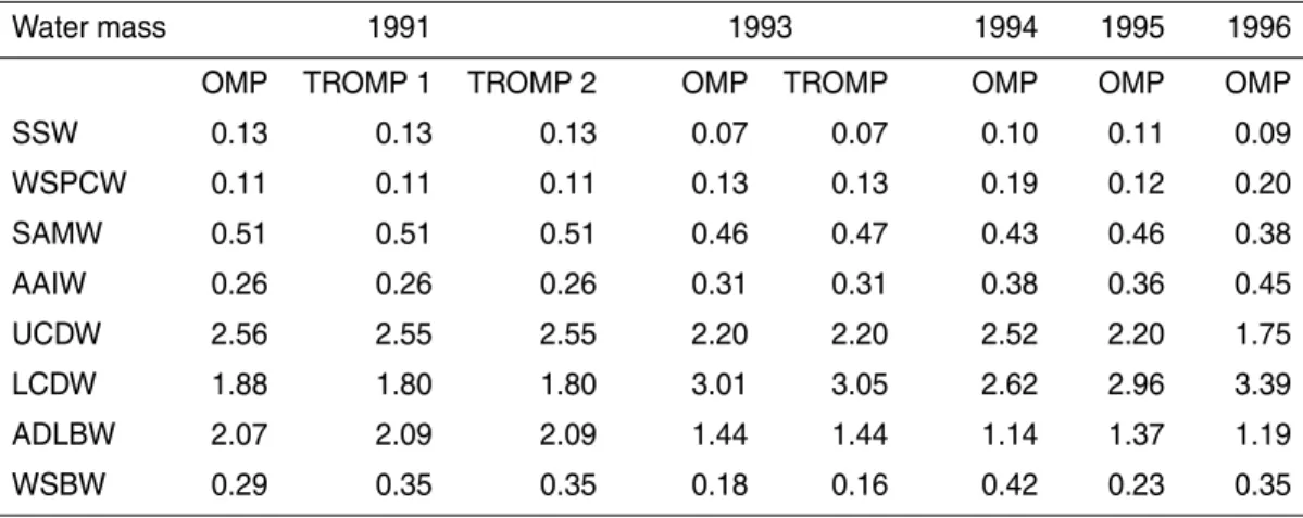
Table VIII shows the result of the comparison. Data for 1994–1996 remain un-changed and are given for reference purposes. It is seen that the calculated volumes
25
are quite insensitive to the changes in the SWT values. The variation in calculated vol-umes is less than 5% and in most cases closer to 1%. The general trend through the years – a reduction of ADBW and UCDW, and an increase of LCDW – is maintained, confirming the findings of Tomczak and Liefrink (2005).
OSD
3, 199–219, 2006Variation of Southern Ocean water mass
volumes M. Tomczak and S. Liefrink Title Page Abstract Introduction Conclusions References Tables Figures J I J I Back Close Full Screen / Esc
Printer-friendly Version Interactive Discussion The conclusion from this study is that the observed large volume variations – an
increase of LCDW of 80% from 1991 to 1996, accompanied by a decrease of UCDW of 46% and a decrease of ADBW of 74% – reflect real physical processes and are not an artefact produced by the basic assumptions of OMP analysis. Although TROMP analysis provides evidence for small changes of SWTs over time, the changes are not
5
large enough to invalidate the result. Tomczak and Liefrink (2005) suggested “heaving” (a change of volume due to variations of the wind stress curl; Bindoff and McDougall, 1994) as the process responsible for the changes in water mass volume. This study tends to confirm that conclusion, although some water mass warming in 1991 and cooling in 1993 cannot be excluded.
10
Could the SWT changes found in 1991 and 1993 be the result of seasonal vari-ability? Water mass formation is most active during winter, when taking oceanographic observations from a research vessel is next to impossible. Seasonal variability can only exceed interannual variability if the Southern Ocean water masses receive significant amounts of freshly formed water during non-winter seasons as well, which is unlikely.
15
If the repeat occupations of SR03 are arranged according to season the sequence is:
January: 1994
March: 1993
August: 1995
September: 1996
October: 1991
The sequence shows that observation sets with SWT values corresponding to the five-year mean (1994, 1995 and 1996) are distributed over all seasons, while the two “anomalous” sections fall into spring and autumn. Taken as an ensemble, the data do
20
not show a systematic seasonal trend. We conclude that the reason for the observed variability of water mass volumes in the Southern Ocean is interannual variability linked to variations in the wind field.
OSD
3, 199–219, 2006Variation of Southern Ocean water mass
volumes M. Tomczak and S. Liefrink Title Page Abstract Introduction Conclusions References Tables Figures J I J I Back Close Full Screen / Esc
Printer-friendly Version Interactive Discussion
Acknowledgements. We thank A. Henry-Edwards for assistance with the programming of the
TROMP routine for the present application. This research was supported in part by a grant from the Australian Antarctic Division.
References
Arbic, B. K. and Owens, W. B.: Climatic warming of Atlantic Intermediate Waters, J. Climate,
5
14, 4091–4108, 2001.
Bindoff, N. L. and McDougall, T. J: Diagnosing climate change and ocean ventilation using hydrographic data, J. Phys. Ocea., 24, 1137–1152, 1994.
Bindoff, N. L. and McDougall, T. J.: Decadal changes along an Indian Ocean section at 32◦S and their interpretation, J. Phys. Ocea. 20, 1207–1221, 2000.
10
Henry-Edwards, A. and Tomczak, M.: Remote detection of water property changes from a time series of oceanographic data, Ocean Science, 2, 11–18, 2005a.
Henry-Edwards, A. and Tomczak, M.: Detecting changes in Labrador Sea Water through a water mass analysis of BATS data, Ocean Science, 2, 19–25, 2005b.
Johnson, G. C. and Orsi, A. H.: Southwest Pacific Ocean water-mass changes between
15
1968/69 and 1990/91, J. Climate 10, 306–316, 1997.
Poole, R. and Tomczak, M.: Optimum Multiparameter analysis of the water mass structure in the Atlantic Ocean thermocline., Deep-Sea I, 46, 1895–1921, 1999.
Rintoul, S. R. and Bullister, J. L.: A late winter hydrographic section from Tasmania to Antarc-tica, Deep-Sea I, 46, 1417–1454, 1999.
20
Rintoul, S. R. and England, M. H.: Ekman transport dominates local air-sea fluxes in driving variability of Subantarctic Mode Water, J. Phys. Ocea. 32, 1308–1321, 2002.
Santoso, A., England, M. H., and Hirst, A. C.: Circumpolar deep water circulation and variability in a coupled climate model, J. Phys. Ocea., 2, 19–25, 2006.
Tomczak, M. and Liefrink, S.: Interannual variations of water mass volumes in the Southern
25
Ocean, J. Atmos. Sci. 10, 31–42, 2005.
OSD
3, 199–219, 2006Variation of Southern Ocean water mass
volumes M. Tomczak and S. Liefrink Title Page Abstract Introduction Conclusions References Tables Figures J I J I Back Close Full Screen / Esc
Printer-friendly Version Interactive Discussion
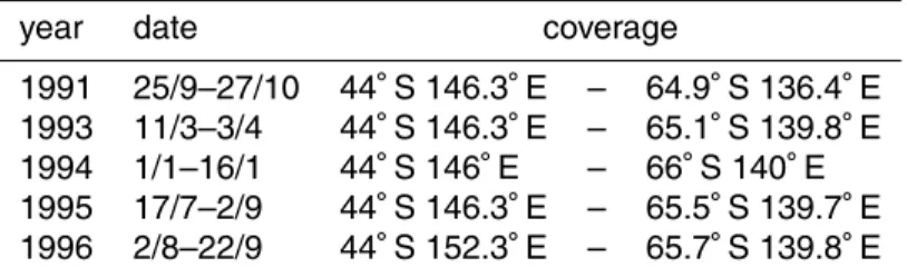
Table 1. SR03 repeat sections.
year date coverage
1991 25/9–27/10 44◦S 146.3◦E – 64.9◦S 136.4◦E 1993 11/3–3/4 44◦S 146.3◦E – 65.1◦S 139.8◦E 1994 1/1–16/1 44◦S 146◦E – 66◦S 140◦E 1995 17/7–2/9 44◦S 146.3◦E – 65.5◦S 139.7◦E 1996 2/8–22/9 44◦S 152.3◦E – 65.7◦S 139.8◦E
OSD
3, 199–219, 2006Variation of Southern Ocean water mass
volumes M. Tomczak and S. Liefrink Title Page Abstract Introduction Conclusions References Tables Figures J I J I Back Close Full Screen / Esc
Printer-friendly Version Interactive Discussion
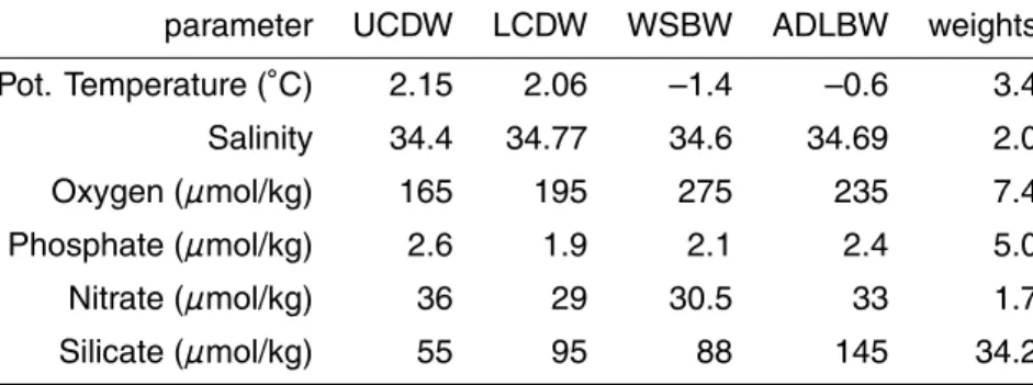
Table 2. Source water type definitions and parameter weights.
parameter UCDW LCDW WSBW ADLBW weights Pot. Temperature (◦C) 2.15 2.06 –1.4 –0.6 3.4 Salinity 34.4 34.77 34.6 34.69 2.0 Oxygen (µmol/kg) 165 195 275 235 7.4 Phosphate (µmol/kg) 2.6 1.9 2.1 2.4 5.0 Nitrate (µmol/kg) 36 29 30.5 33 1.7 Silicate (µmol/kg) 55 95 88 145 34.2 212
OSD
3, 199–219, 2006Variation of Southern Ocean water mass
volumes M. Tomczak and S. Liefrink Title Page Abstract Introduction Conclusions References Tables Figures J I J I Back Close Full Screen / Esc
Printer-friendly Version Interactive Discussion
Table 3. Difference between potential temperature Θ (◦C) determined through the second
TROMP analysis run and the values given in Table 2. Water Mass Year
1991 1993 1994 1995 1996 UCDW 0.0786 –0.0678 0.0079 0.0016 0.0016 LCDW 0.0725 –0.0575 0.0104 0.0098 0.0088 ADLBW 0.0179 –0.0417 -0.0004 –0.0043 0.0004 WSBW 0.0789 –0.0581 0.0102 –0.0079 –0.0103
OSD
3, 199–219, 2006Variation of Southern Ocean water mass
volumes M. Tomczak and S. Liefrink Title Page Abstract Introduction Conclusions References Tables Figures J I J I Back Close Full Screen / Esc
Printer-friendly Version Interactive Discussion
Table 4. Parameter residuals for 1993 when potential temperature is allowed to vary in all water
masses.
Pot. Tem- Salinity Oxygen Phosphate Nitrate Silicate perature (◦C) (µmol/kg) (µmol/kg) (µmol/kg) (µmol/kg) after one TROMP run 19.64 –0.1395 1.5046 0.4562 –0.3372 0.0709 after six iterations –0.3600 –0.1379 1.4294 0.4033 –0.3532 0.0678
OSD
3, 199–219, 2006Variation of Southern Ocean water mass
volumes M. Tomczak and S. Liefrink Title Page Abstract Introduction Conclusions References Tables Figures J I J I Back Close Full Screen / Esc
Printer-friendly Version Interactive Discussion
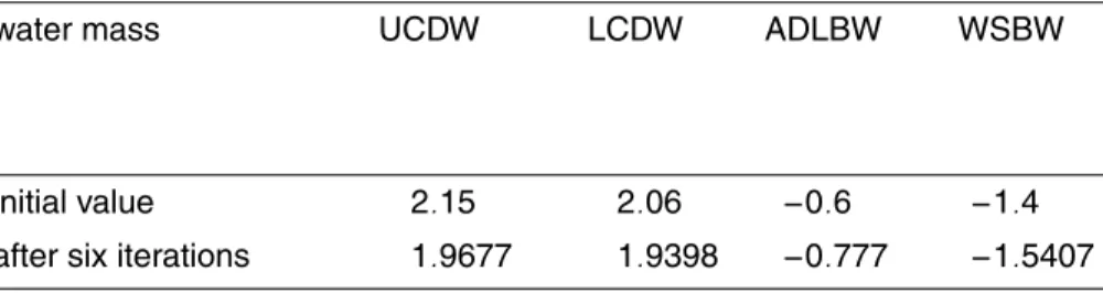
Table 5. Potential temperature (◦C) In the source regions of the four deep water masses corre-sponding to the sixth iteration of Table 4.
water mass UCDW LCDW ADLBW WSBW
initial value 2.15 2.06 −0.6 −1.4 after six iterations 1.9677 1.9398 −0.777 −1.5407
OSD
3, 199–219, 2006Variation of Southern Ocean water mass
volumes M. Tomczak and S. Liefrink Title Page Abstract Introduction Conclusions References Tables Figures J I J I Back Close Full Screen / Esc
Printer-friendly Version Interactive Discussion
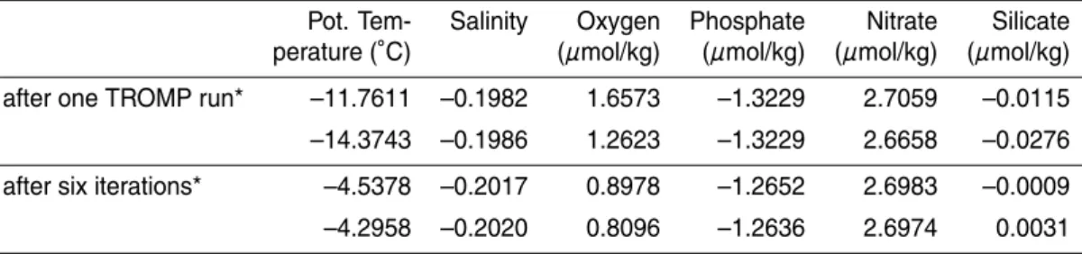
Table 6. Parameter residuals for 1991 when potential temperature and oxygen are allowed to
vary in all water masses.
Pot. Tem- Salinity Oxygen Phosphate Nitrate Silicate perature (◦C) (µmol/kg) (µmol/kg) (µmol/kg) (µmol/kg) after one TROMP run* –11.7611 –0.1982 1.6573 –1.3229 2.7059 –0.0115 –14.3743 –0.1986 1.2623 –1.3229 2.6658 –0.0276 after six iterations* –4.5378 –0.2017 0.8978 –1.2652 2.6983 –0.0009 –4.2958 –0.2020 0.8096 –1.2636 2.6974 0.0031 * The first value is obtained when potential temperature is varied first, the second value when oxygen is varied first.
OSD
3, 199–219, 2006Variation of Southern Ocean water mass
volumes M. Tomczak and S. Liefrink Title Page Abstract Introduction Conclusions References Tables Figures J I J I Back Close Full Screen / Esc
Printer-friendly Version Interactive Discussion
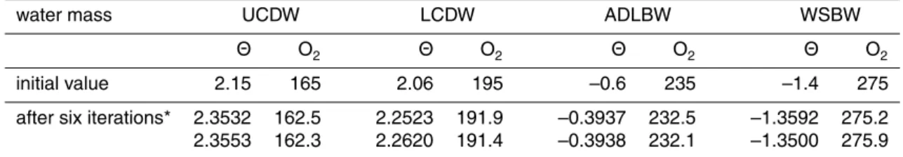
Table 7. Potential temperatureΘ (◦C) and oxygen O2 (µmol/kg) in the source regions of the
four deep water masses corresponding to the sixth iteration of Table 6.
water mass UCDW LCDW ADLBW WSBW
Θ O2 Θ O2 Θ O2 Θ O2
initial value 2.15 165 2.06 195 –0.6 235 –1.4 275 after six iterations* 2.3532 162.5 2.2523 191.9 –0.3937 232.5 –1.3592 275.2 2.3553 162.3 2.2620 191.4 –0.3938 232.1 –1.3500 275.9
* The first value is obtained when potential temperature is varied first, the second value when oxygen is varied first.
OSD
3, 199–219, 2006Variation of Southern Ocean water mass
volumes M. Tomczak and S. Liefrink Title Page Abstract Introduction Conclusions References Tables Figures J I J I Back Close Full Screen / Esc
Printer-friendly Version Interactive Discussion
Table 8. Water mass volumes for a 1-m wide strip along section SR03 (109m2).
OMP= volumes determined by Tomczak and Liefrink (2005); TROMP = volumes determined in this paper. TROMP 1 is the run in which potential temperature is varied first; in TROMP 2 oxygen is varied first.
Water mass 1991 1993 1994 1995 1996 OMP TROMP 1 TROMP 2 OMP TROMP OMP OMP OMP SSW 0.13 0.13 0.13 0.07 0.07 0.10 0.11 0.09 WSPCW 0.11 0.11 0.11 0.13 0.13 0.19 0.12 0.20 SAMW 0.51 0.51 0.51 0.46 0.47 0.43 0.46 0.38 AAIW 0.26 0.26 0.26 0.31 0.31 0.38 0.36 0.45 UCDW 2.56 2.55 2.55 2.20 2.20 2.52 2.20 1.75 LCDW 1.88 1.80 1.80 3.01 3.05 2.62 2.96 3.39 ADLBW 2.07 2.09 2.09 1.44 1.44 1.14 1.37 1.19 WSBW 0.29 0.35 0.35 0.18 0.16 0.42 0.23 0.35 218
OSD
3, 199–219, 2006Variation of Southern Ocean water mass
volumes M. Tomczak and S. Liefrink Title Page Abstract Introduction Conclusions References Tables Figures J I J I Back Close Full Screen / Esc
Printer-friendly Version Interactive Discussion
EGU
contains five complete transects for the years 1991 – 1996. Table I gives the dates of
individual transects. The WOCE data provided potential temperature, salinity,
oxygen, phosphate, nitrate and silicate as parameters for water mass analysis.
Figure 1: Location of WOCE repeat section SR03. Squares indicate station locations
occupied during 1991 – 1996. The four stations west of 140°E were occupied in 1991.
Table I: SR03 Repeat Sections
year date coverage
1991
25/9 – 27/10
44°S 146.3°E – 64.9°S 136.4°E
1993
11/3 – 3/4
44°S 146.3°E – 65.1°S 139.8°E
1994
1/1 – 16/1
44°S 146°E
– 66°S 140°E
1995
17/7 – 2/9
44°S 146.3°E – 65.5°S 139.7°E
1996
2/8 – 22/9
44°S 152.3°E – 65.7S 139.8°E
The previous analysis used data interpolated vertically onto a 50m grid that covered a
depth range 50 – 4250 m. The surveyed area was restricted to a common latitude
range between 44°42.2'S and 64°53.3'S and a common bathymetry for all years.
Water mass volumes were determined by integration over the relative contributions of
each water mass.
In contrast to the earlier study, which determined the relative contributions through
OMP analysis, a further development of the method called Time-Resolving Optimum
Multiparameter (TROMP) analysis is used here to determine interannual variations in
Fig. 1. Location of WOCE repeat section SR03. Squares indicate station locations occupied
during 1991–1996. The four stations west of 140◦E were occupied in 1991.