HAL Id: hal-00409302
https://hal.archives-ouvertes.fr/hal-00409302
Submitted on 18 Jun 2021
HAL is a multi-disciplinary open access
archive for the deposit and dissemination of
sci-entific research documents, whether they are
pub-lished or not. The documents may come from
teaching and research institutions in France or
abroad, or from public or private research centers.
L’archive ouverte pluridisciplinaire HAL, est
destinée au dépôt et à la diffusion de documents
scientifiques de niveau recherche, publiés ou non,
émanant des établissements d’enseignement et de
recherche français ou étrangers, des laboratoires
publics ou privés.
High-frequency non-tidal ocean loading effects on
surface gravity measurements
Jean-Paul Boy, Florent Lyard
To cite this version:
Jean-Paul Boy, Florent Lyard. High-frequency non-tidal ocean loading effects on surface gravity
measurements. Geophysical Journal International, Oxford University Press (OUP), 2008, 175 (1),
pp.35-45. �10.1111/j.1365-246X.2008.03895.x�. �hal-00409302�
GJI
Geo
desy
,
p
otential
field
and
a
pplied
g
eophysics
High-frequency non-tidal ocean loading effects on surface gravity
measurements
Jean Paul Boy
1and Florent Lyard
21EOST-IPGS (UMR 7516 CNRS-ULP), 5 rue Rene Descartes, 67084 Strasbourg, France. E-mail: [email protected] 2LEGOS (UMR 5566), 14 Avenue Edouard Belin, 31400 Toulouse, France
Accepted 2008 June 23. Received 2008 June 23; in original form 2008 March 12
S U M M A R Y
We model atmospheric and non-tidal oceanic loading effects on surface gravity variations, us-ing global surface pressure field provided by the European Centre for Medium-range Weather Forecasts (ECMWF), and sea surface height from the Toulouse Hydrodynamic Unstructured Grid Ocean model (HUGO-m) barotropic ocean model. We show the improvement in terms of reduction of variance of 15 different superconducting gravimeters of the worldwide Global Geodynamics Project (GGP) network, compared to the classical inverted barometer assump-tion.
We also study two storm surges over the Western European Shelf in 2000 and 2003. We compare the HUGO-m sea surface height variations to various tide gauges measurements as well as the induced loading effects to the computations of Fratepietro et al., using the Proudman Storm Surge model, for the Membach (Belgium) station. The agreement between modelled ocean loading and gravity observations is largely improved when using a global atmospheric loading correction, compared to the classical local approach. The remaining discrepancies are mainly due to hydrological loading contributions.
Key words: Sea level change; Time variable gravity.
1 I N T R O D U C T I O N
Atmospheric loading is, besides solid Earth tides and ocean tidal loading, one of the major sources of surface gravity perturbations over a wide frequency domain (see, for example, Boy et al. 2002). With the help of global atmospheric data sets provided by meteoro-logical centres and Green’s function formalism (Farrell 1972), the atmospheric loading can easily computed (Boy et al. 2002) and can reduce gravity residuals over a large frequency band (from typically a few days to 100 days). The main limitation of these computations is the assumption of a simple ocean response to pressure forcing: the ‘non-inverted barometer’ (NIB) or the ‘inverted barometer’ (IB) hypotheses (Wunsch & Stammer 1997). In a previous study (Boy
et al. 2002), we have shown that the NIB assumption cannot be a
valid model for estimating the ocean response to pressure forcing. We here show the improvement in reduction of gravity residuals, by adding to our global atmospheric loading computations, the effects due to the dynamic barotropic ocean response to air pressure and wind forcing.
Non-tidal oceanic loading effects on superconducting gravime-ters have already been studied by, for example, Virtanen (2004) and Zerbini et al. (2004). However, they were looking at lower frequencies (typically seasonal timescales). For these periods, the oceanic circulation is mostly forced by heat and fresh water fluxes and winds, and the oceans cannot be consider as barotropic. The high-frequency barotropic oceanic loading effects on surface
grav-ity have been modelled by Fratepietro et al. (2006) for the station of Membach (Belgium) and for a 2 week period, corresponding to a storm surge occuring over the North Sea. However, they suggested to use non-tidal ocean models, forced by air pressure and winds, such as MOG2D (Carr`ere & Lyard 2003), for better non-tidal ocean loading corrections on gravity measurements.
In this paper, we are adding to our atmospheric loading esti-mates, using surface pressure field provided by the European Centre for Medium-Range Weather Forecasts (ECMWF), non-tidal ocean loading computed using the Toulouse Hydrodynamic Unstructured Grid Ocean model (HUGO-m) (MOG2D follow-on) barotropic ocean model forced by ECMWF pressure and wind fields (Carr`ere & Lyard 2003). This model is also currently used for the Gravity Recovery And Climate Experiment (GRACE) (Lemoine et al. 2007) and radar altimetry processing.
Other ocean models forced by air pressure and winds are also currently available, thanks to the GRACE project (Flechtner 2005): the so-called PPHA (Hirose et al. 2001) barotropic, and the Ocean Model for Circulation and Tides (OMCT) (Dobslaw & Thomas 2005) baroclinic ocean models. However their spatial resolution (1.125◦for PPHA and 1.875◦for OMCT) do not allow a precise es-timation of oceanic mass variations over continental shelves, which have been shown to have a significant contribution to surface grav-ity changes (Fratepietro et al. 2006). On the other hand, the lack of the Arctic ocean in the PPHA model do not allow to model high frequency non-tidal ocean loading in Ny-Alesund (Svalbard), one
of the stations of the Global Geodynamic Project (GGP) network (Crossley et al. 1999).
As we are studying the high frequency surface gravity variations (periods smaller than typically a few months), we choose to model the atmospheric loading effects using only surface pressure data fol-lowing Merriam (1992) and Boy et al. (2002), and not the complete 3-D structure of the atmosphere, as Neumeyer et al. (2004) showed that the differences between the 2-D and 3-D approaches are larger at seasonal timescales (differences of about 1μGal).
In Section 2, we present the computations of atmospheric and oceanic loading effects, from surface pressure field provided by ECMWF, and sea surface height variations from the HUGO-m barotropic ocean model. In Section 3, we show the reduction of gravity residuals using HUGO-m, compared to the classical NIB and IB approaches. Section 4 is devoted to the study of some storm surges occurring in the North Sea, with a comparison with Fratepi-etro et al. (2006). Discussion and concluding remarks are given in Section 5.
2 AT M O S P H E R I C A N D O C E A N I C L O A D I N G C O M P U T AT I O N S
2.1 Comparison between the IB assumption and the barotropic model
We are using 6-hourly sea surface height outputs of the HUGO-m barotropic ocean HUGO-model, forced by 6-hourly ECMWF surface pressure and winds, given on a regular 0.5◦global grid, obtained by an interpolation of the native finite element grid (Carr`ere & Lyard 2003).
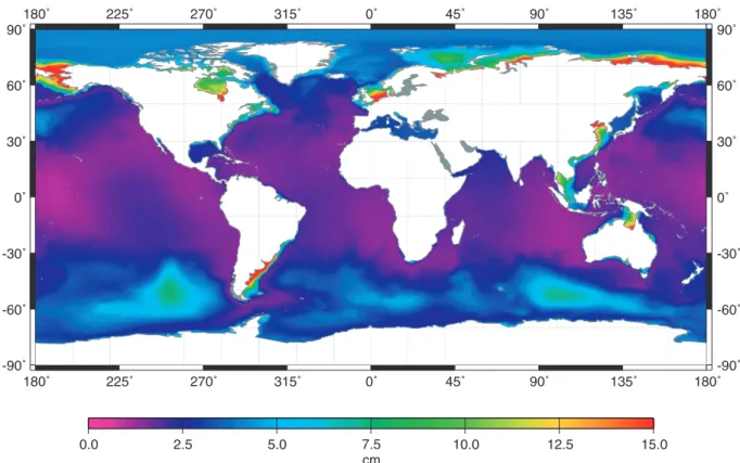
Fig. 1 shows the root mean square (rms) differences between the IB assumption and HUGO-m sea surface height, computed for the
Figure 1. The rms differences (in cm) between the inverted barometer assumption and HUGO-m, computed for the 1997–2006 period.
2000–2006 period. The larger differences occur over shallow water regions, such as the European, the Patagonia shelves, and along the Arctic Sea coast; they can reach up to 25 cm. Due to the large pressure and wind forcing, the differences can be as large as 10 cm around Antarctica.
Fig. 1 also exhibits the lack of some small enclosed or semi-enclosed basins (shown in grey) in HUGO-m. As Virtanen (2004) showed, there is a strong correlation between Mets¨ahovi (Finland) gravity residuals and tide gauge measurements in the Baltic Sea. The lack of the Baltic Sea in HUGO-m may lead us to a lower reduction of residuals variance for this station, compared to other European instruments.
2.2 Green’s function formalism
Surface gravity variations are computed through a convolution of Green’s functions (Farrell 1972) and surface pressure field provided by the ECMWF or barotropic sea surface height from the HUGO-m model. The computation of the atmospheric loading effects follows Boy et al. (2002), that is, the atmospheric thickness is not neglected, but the air density variations with height are supposed to be only function of the surface pressure (Merriam 1992). The ocean loading effects are modelled as a thin-layer process.
The global pressure field are replaced by the local pressure mea-surements colocated with the gravimeter for a local cell with a radius 0.1◦around the gravimeters. The ECMWF Reanalyis ERA-40 project (Uppala et al. 2005) ended in 2002 August, unlike the NCEP Reanalysis (Kalnay et al. 1996) with data available up to now almost in real time, therefore we had to combine data sets from different operational models. We also take the advantage of the 4-D variational assimilation operational implementation at the ECMWF (Rabier et al. 2000), starting in 1997 December to use surface pressure field data with a temporal resolution of 3 hr.
For the ocean loading effects, sea height variations are depending on the choice of the ocean response to pressure forcing:
(i) h(θ, λ, t) = 0, for a non-inverted ocean response to pressure forcing.
(ii) h(θ, λ, t) = −p(θ,λ,t)− ˜p(t)ρ
wg0 (where ˜p(t) is the mean air
pres-sure over the oceans), for an IB hypothesis.
(iii) h(θ, λ, t) is the output of the barotropic models forced by pressure and winds, if the dynamic ocean response to pressure is taken into account.
3 R E D U C T I O N O F S U R FA C E G R AV I T Y R E S I D UA L S
3.1 Processing of gravity data
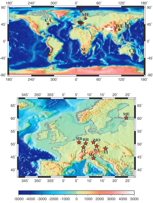
We extract from the GGP global network (Crossley et al. 1999), 15 superconducting gravimeters (see Fig. 2 for their location). Raw
Figure 2. Location of the different superconducting gravimeters of the Global Geodynamics Project (GGP) network.
1-min gravity and pressure are classically pre-processed following Crossley et al. (1993), and then decimated to hourly samples.
Gravity are then corrected from polar motion and length-of-day induced effects (Wahr 1985), using EOPC04 series from the Inter-national Earth Rotation Service (IERS), assuming an elastic Earth and an equilibrium pole tide, including self-attraction and loading terms (Agnew & Farrell 1978). Long period tides (solid Earth and ocean tidal loading) are removed using Dehant et al. (1999) theoret-ical gravimetric factors and NAO99b ocean tide model (Matsumoto
et al. 2000). The different atmospheric and oceanic loading
cor-rections, that is, local pressure correction (barometric admittance), ECMWF–NIB, ECMWF–IB and ECMWF and HUGO-m, are then applied, before performing a tidal analysis using the ETERNA pack-age (Wenzel 1997) in order to remove daily and subdaily solid Earth tide and ocean tidal loading contributions.
We choose not to correct for continental hydrology loading ef-fects, as we have only access to global soil moisture and snow
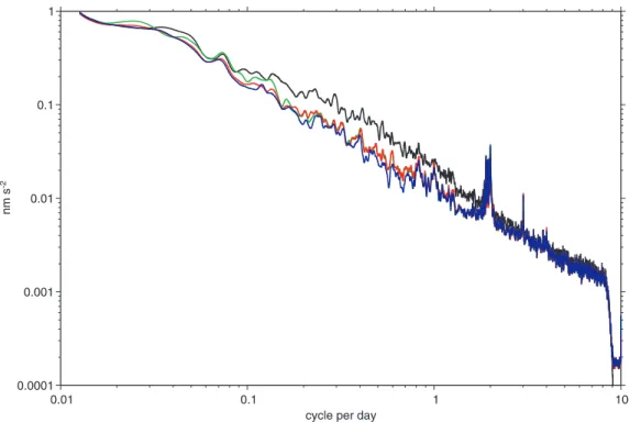
Figure 3. Spectrum of gravity residuals for the SG CO26 installed in Strasbourg, with the different atmospheric and oceanic loading correction, that is, local pressure correction (black), ECMWF–NIB (green), ECMWF–IB (red) and ECMWF+HUGO-m (blue).
models, such as Global Land Data Assimilation System (GLDAS) (Rodell et al. 2004). Due to their spatial sampling, they are not always able to recover all the short wavelength features near the gravimeters (Boy & Hinderer 2006). In order to improve hydrolog-ical loading computations, local measurements would be required (Van Camp et al. 2006), but they are not currently available for all instruments.
3.2 Results from tidal analyses
We compare the gravity residuals with the different atmospheric and oceanic corrections, and for the 15 superconducting gravime-ters. Fig. 3 shows the spectrum of gravity residuals for the CO26 gravimeter, installed in Strasbourg (France), computed for the 1997– 2007 period. We retrieve a similar result as Boy et al. (2002) using ECMWF rather than NCEP Reanalysis (Kalnay et al. 1996) sur-face pressure field, that is, that the IB hypothesis allows a reduction of gravity residuals compared to the local pressure correction and the NIB assumption, for periods up to a few months. However the differences between the global pressure correction using the ECMWF fields and the local pressure corrections are larger than using the NCEP Reanalysis fields, because of their higher spatial (up to approximatively 0.25◦in 2006) and temporal (3 hr after 1997 December) sampling (2.5◦ and 6 hr for NCEP Reanalysis). Some tidal signals in the diurnal and semi-diurnal bands are still left in the residuals, as well as a peak at S3 (8 hr) period.
The use of the barotropic HUGO-m ocean model, forced by ECMWF pressure and winds, allows a reduction of the gravity resid-uals for the Strasbourg instrument, for periods between typically one day and a few months. The improvement in term of reduction of residuals comes mainly from the modelling of the ocean variability over the North Sea and the Northwestern European shelf, as the
departure from the IB assumption are larger over shallow water regions (see Fig. 1).
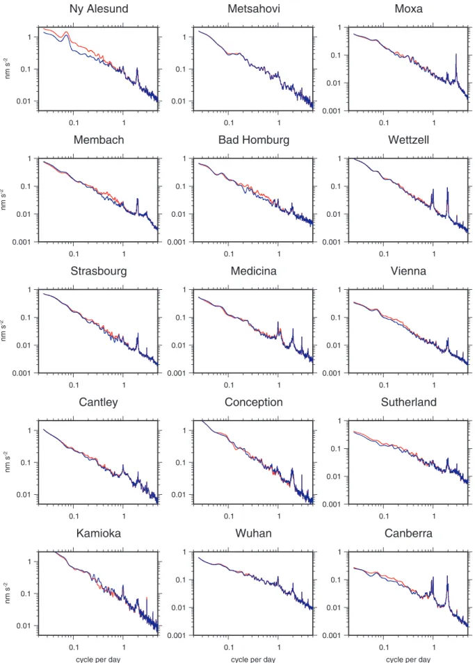
As Boy et al. (2002) results are confirmed, we choose to plot on Fig. 4, gravity residuals with the ECMWF− IB and ECMWF + HUGO-m loading corrections for all superconducting gravimeters. Except for Kamioka (Japan) and Mets¨ahovi (Finland) instruments, the residuals are lower with HUGO-m, compared to the IB assump-tion, for period between typically 1 d and 20–50 d. This is partic-ularly true for Ny-Alesund (Svalbard), Sutherland (South Africa) and Canberra (Australia) which are close to coasts, and at high lat-itudes, that is, where the differences between the IB and HUGO-m are larger (see Fig. 1). Kamioka is the newest station (installed in 2004), but is an old version of superconducting gravimeter, such as the instrument installed in Mets¨ahovi. For this gravimeter, the lack of the Baltic Sea in HUGO-m might be the reason of similar residuals with the two atmospheric and oceanic loading corrections.
Table 1 shows the mean amplitude of gravity residuals with the ECMWF-IB and ECMWF+HUGO-m loading corrections, for six different frequency bands: periods, respectively, larger than 1000 days, between 1000 and 250 days, between 50 and 250 days, between 10 and 50 days, 2 and 10 days and finally between 6 hr and 2 days. As shown on Fig. 4, non-tidal ocean loading correc-tions using HUGO-m, allow a systematic and significant reduction (10 per cent and more) of gravity residuals for period between a few days and about 50 days, compared to the IB assumption. For long (larger than 250 days) and short (smaller than 2 d) periods, there is no improvement in terms of reduction of the variance of gravity residuals.
4 E X A M P L E S O F S T O R M S U R G E S I N E U R O P E
Over continental shelves, air pressure and winds can cause large sea surface height variations, known as storm surges. Their amplitude
Figure 4. Spectrum of gravity residuals for all superconducting gravimeters, with the ECMWF-IB (red) and ECMWF+HUGO-m (blue) loading corrections.
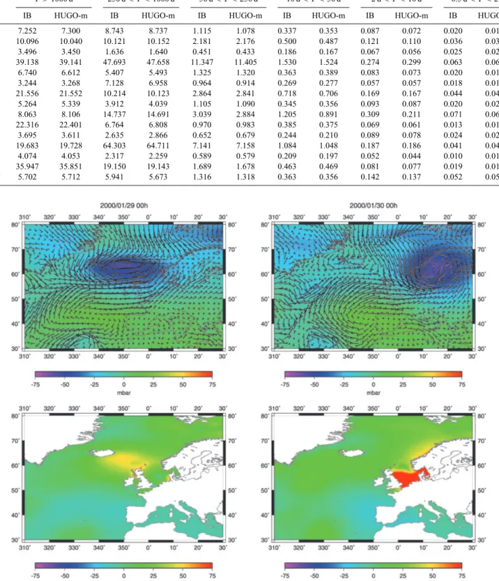
Table 1. Amplitude of gravity residuals using ECMWF–IB and ECMWF+HUGO-m loading corrections, as a function of the period band.
T> 1000 d 250 d< T < 1000 d 50 d< T < 250 d 10 d< T < 50 d 2 d< T < 10 d 0.5 d< T < 2 d
IB HUGO-m IB HUGO-m IB HUGO-m IB HUGO-m IB HUGO-m IB HUGO-m
BH 7.252 7.300 8.743 8.737 1.115 1.078 0.337 0.353 0.087 0.072 0.020 0.018 CA 10.096 10.040 10.121 10.152 2.181 2.176 0.500 0.487 0.121 0.110 0.036 0.036 CB 3.496 3.450 1.636 1.640 0.451 0.433 0.186 0.167 0.067 0.056 0.025 0.026 KA 39.138 39.141 47.693 47.658 11.347 11.405 1.530 1.524 0.274 0.299 0.063 0.067 MB 6.740 6.612 5.407 5.493 1.325 1.320 0.363 0.389 0.083 0.073 0.020 0.017 MC 3.244 3.268 7.128 6.958 0.964 0.914 0.269 0.277 0.057 0.057 0.018 0.017 ME 21.556 21.552 10.214 10.123 2.864 2.841 0.718 0.706 0.169 0.167 0.044 0.044 MO 5.264 5.339 3.912 4.039 1.105 1.090 0.345 0.356 0.093 0.087 0.020 0.020 NY 8.063 8.106 14.737 14.691 3.039 2.884 1.205 0.891 0.309 0.211 0.071 0.068 ST 22.316 22.401 6.764 6.808 0.970 0.983 0.385 0.375 0.069 0.061 0.013 0.012 SU 3.695 3.611 2.635 2.866 0.652 0.679 0.244 0.210 0.089 0.078 0.024 0.024 TC 19.683 19.728 64.303 64.711 7.141 7.158 1.084 1.048 0.187 0.186 0.041 0.044 VI 4.074 4.053 2.317 2.259 0.589 0.579 0.209 0.197 0.052 0.044 0.010 0.010 WE 35.947 35.851 19.150 19.143 1.689 1.678 0.463 0.469 0.081 0.077 0.019 0.018 WU 5.702 5.712 5.941 5.673 1.316 1.318 0.363 0.356 0.142 0.137 0.052 0.052
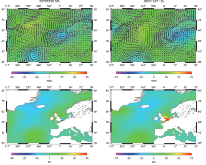
Figure 5. Surface pressure, winds (ECMWF) and sea surface height (HUGO-m) for the 2000 January 29 and 30, corresponding to the storm surge studied by Fratepietro et al. (2006).
can reach several metres in the North Sea. Fratepietro et al. (2006) compared gravity residuals at the Membach station to the load-ing computed with the Proudman Oceanographic Laboratory storm surge model, for an event in 2000 January–February (see Fig. 5).
We are extending this previous study to another storm surge which occurred in 2003 December, and to all available supercon-ducting gravimeters installed in western Europe, and not only to the Membach instrument as it was done by Fratepietro et al. (2006).
Figure 6. Same as Fig. 5, but for the 2003 December 20 and 21.
Despite its different temporal (6-hourly instead of hourly samples) and spatial resolution (0.5◦instead of 12 km), we are still using the HUGO-m ocean model, instead of the POL barotropic model. How-ever, the spatial resolution of the finite element grid of HUGO-m is about 20 km along the European coasts. Before comparing loading estimates to gravity residuals, we are first showing the agreement between HUGO-m sea surface height variations with several tide gauges along the North Sea coasts.
4.1 Comparison of HUGO-m sea height variations with tide gauges
Fig. 5 shows the surface pressure and wind variations from ECMWF, and the sea surface height variations from HUGO-m, for the 2000 January 29 and 30, showing the storm surge in the North Sea studied by Fratepietro et al. (2006). Due to the wind forcing, the amplitude of the sea surface height variations reached about 1 m, on the Belgian coasts the 30th of January.
The 2003 December storm surge is also shown in Fig. 6. Although the maximum amplitude is also larger than 1 m along the North Sea coasts, the spatial extend is much smaller compared to the 2000 event.
We extracted from various networks eight different tide gauge records, along the North Sea coasts. Figs 7 and 8 the good
agree-ment between HUGO-m sea surface height and detided tide gauge measurements for the 2000 and, respectively, 2003 storm surges. Despite the spatial (0.5◦) and temporal (6 hr) sampling, HUGO-m barotropic ocean model is able to simulate the small wavelength features of the two surges. It allows us therefore to use HUGO-m model to estimate gravity loading effects, and not only dedicated storm surge models, such as the POL model used by Fratepietro
et al. (2006).
4.2 Gravity variations
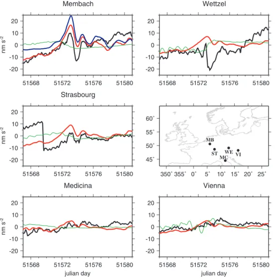
Fig. 9 shows the gravity residuals (corrected for tides, atmo-spheric loading and polar motion) for five different superconducting gravimeters in Europe, as well as the non-tidal ocean loading mod-elled with HUGO-m. For the Membach stations, we also plot the loading effects using the POL model (Fratepietro et al. 2006). In green is also shown the global hydrology loading effects (Boy & Hinderer 2006), estimated from soil-moisture and snow from the ECMWF Reanalysis (ERA40) project (Uppala et al. 2005). For Membach station, the agreement between gravity observations and loading estimates is better than Fratepietro et al. (2006), because of the different estimation of atmospheric loading effects. We com-pute the atmospheric loading using 3-hourly global surface pressure field provided by the ECMWF, whereas Fratepietro et al. (2006)
Figure 7. Comparison of HUGO-m sea surface height variations (red) with several tide gauges (black) along the North Sea coasts, for 2000 January and February.
Figure 8. Same as Fig. 7, but for 2003 December.
Figure 9. Gravity residuals (black) for various superconducting gravimeters in Europe and non-tidal ocean loading from HUGO-m model (red), the POL storm surge model (blue) and global hydrology (ECMWF Reanalysis) loading (green) for 2000 January and February.
removed atmospheric effects using only local air pressure and a linear admittance factor (Warburton & Goodkind 1977).
The non-tidal ocean loading amplitude decreases with the dis-tance to the North Sea coasts, but still reaches about 10 nm s−2 (1μgal) in Vienna. The large offset for Strasbourg the 2000 Jan-uary 26 (Julian day equal to 51569) may be due by instrument noise, but not by a geophysical induced signal. Storms are often linked with heavy rainfall, but the ERA-40 soil-moisture model does not shown large hydrological induced loading. However, the coarse resolution of the model (1.125◦) may not be adequate to represent small wavelength and rapid rainfall events, and therefore, soil moisture changes. This is one of the reason to extend this study to the 2003 December storm surge, in addition to the larger number of gravimeters at this time.
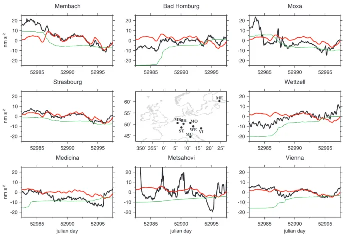
Fig. 10 shows the gravity residuals for eight instruments, the non-tidal ocean loading and the global hydrology loading using the state-of-the-art GLDAS (Rodell et al. 2004) hydrology model. Its spatial (0.25◦) and temporal (3 hr) resolutions should be more adequate to estimate the soil-moisture changes associated with the storm. For Membach, Bad-Homburg, Strasbourg and Wettzell, it is clear that HUGO-m and GLDAS can explain the gravity variations for these two weeks. For the Mets¨ahovi station, the large gravity variations cannot be explained, but HUGO-m does not include the Baltic Sea.
As shown by Virtanen & M¨akinen (2003) and Virtanen (2004), there is indeed a strong correlation between Mets¨ahovi gravity residuals and tide gauge measurements in the Baltic sea. New versions of HUGO-m model now include the semi-enclosed basins, such as the Baltic and the Black Seas.
Table 2 gives the correlation coefficients between gravity resid-uals, non-tidal ocean loading, and hydrology loading for the two storm surges. For the 2000 January–February event, the correlation between gravity residuals and the ocean loading is higher than 0.5. The negative correlation for Strasbourg is due to the negative jump at the beginning of the time-series. Hydrological contribution esti-mated with ECMWF Reanalysis soil-moisture and snow models is correlated with gravity residuals only for Wettzell station.
As the 2003 December storm surge is smaller in amplitude than the 2000 January–February surge, the correlation between gravity residuals and HUGO-m estimated loading is also smaller. The cor-relation is larger than 0.5 only for Membach, Strasbourg and Vienna instruments. Another interesting result is the higher correlation be-tween gravity and hydrology loading, estimated with GLDAS.
An improvement of the hydrology loading estimates would re-quire, in addition to the global fields, local measurements of soil water content, as shown by Van Camp et al. (2006), but this is not the aim of the paper. However the differences between the two
Figure 10. Same as Fig. 9, but for 2003 December, and GLDAS hydrology model (green).
Table 2. Correlation coefficients between gravity residuals, non-tidal ocean loading and hydrology loading, for the 2000 January–February and 2003 December storm surges.
2000 January–February 2003 December
Residual and HUGO-m Residual and ERA40 HUGO-m and ERA40 Residual and HUGO-m Residual and GLDAS HUGO-m and GLDAS
BH 0.36 0.70 −0.23 MB 0.83 −0.42 −0.52 0.55 0.77 0.20 MC 0.52 −0.34 −0.22 0.48 0.49 −0.02 ME 0.71 0.73 0.86 0.25 −0.53 −0.39 MO 0.34 0.46 0.21 ST −0.33 −0.16 −0.04 0.82 0.19 0.13 VI 0.81 −0.19 −0.19 0.69 −0.52 −0.32 WE 0.59 0.61 0.65 0.13 0.67 −0.31
approaches would not change the agreement between gravity resid-uals and the non-tidal ocean loading effects, estimated with HUGO-m, for the 2003 December storm surge. However, ERA-40 resolution may not be sufficient to model the rapid and small wavelength soil moisture variations for 2000 January–February.
5 D I S C U S S I O N A N D C O N C L U S I O N
We have shown that HUGO-m (Carr`ere & Lyard 2003) barotropic ocean model allows a systematic reduction of gravity residuals for all superconducting gravimeters, compared to the IB assumption, as previous used by Boy et al. (2002) in their atmospheric loading estimates. As the dynamic ocean response to pressure forcing does not differ from the static IB model at low frequencies, there is no decrease of gravity residuals for periods exceeding typically 50–100 d. On the other hand, although the departure from the IB
increases with the frequency, there is no evidence of reduction of gravity residuals for periods lower than a few days. Periods below typically 1 d should be improved using 3-hourly ECMWF pressure and winds, instead of 6-hourly samples, when forcing HUGO-m barotropic ocean model.
At seasonal timescales, the atmospheric and non-tidal oceanic loading effects are not anymore the main source of gravity vari-ations. They are mainly due to continental hydrology (Boy & Hinderer 2006), which can be modelled using global hydrology models (soil moisture and snow) such as GLDAS (Rodell et al. 2004), and also local measurements (Van Camp et al. 2006).
Because of their sensitivity, and their vicinity to the coasts (usu-ally distances less than 1000 km), superconducting gravimeter pro-cessing requires a model with a high spatial sampling rate, such as HUGO-m. Models like PPHA (Flechtner 2005) with resolution larger than 100 km cannot be used to correct gravity observations
from non-tidal oceanic loading, as they are not able to represent correctly sea height variations over shallow water regions, although the differences between these models are quite small on open oceans.
However, HUGO-m ocean model allows a precise estimation of short period non-tidal ocean loading over the North Sea, in the case of large storm surges. The comparison with the previous study by Fratepietro et al. (2006) shows the importance of a precise atmo-spheric correction, using global pressure field instead of the local pressure alone, for an accurate estimation of gravity residuals, even at high frequencies. As storms are associated with rapid variations of the vertical profile of temperature, an improvement of the at-mospheric loading estimates will require to compute the complete 3-D atmospheric correction (Neumeyer et al. 2004), as it is done operationally for space gravity mission processing (Boy & Chao 2005).
A C K N O W L E D G M E N T S
We thank all the GGP members for providing high quality minute gravity and pressure data. We also thank European Sea Level Service (ESEAS) (http://www.eseas.org/), British Oceanographic Data Cen-ter (BODC) (http://www.bodc.ac.uk/) and Syst`eme d’Observation du Niveau des Eaux Littorales (SONEL) (http://www.sonel.org/) for providing the tide gauge measurements.
R E F E R E N C E S
Agnew, D.C. & Farrell, W.E., 1978. Self-consistent equilibrium ocean tides,
Geophys. J. R. astr. Soc., 55, 171–181.
Boy, J.-P. & Chao, B.F., 2005. Precise evaluation of atmospheric loading ef-fects on Earth’s time-variable gravity field, J. geophys. Res., 110, B08412, doi:10.1029/2002JB002333.
Boy, J.-P. & Hinderer, J., 2006. Study of the seasonal gravity signal in superconducting gravimeter data, J. Geodyn., 41, 227–233.
Boy, J.-P., Gegout, P. & Hinderer, J., 2002. Reduction of surface gravity data from global atmospheric pressure loading, Geophys. J. Int., 149, 534–545. Carr`ere, C. & Lyard, F., 2003. Modeling the barotropic response of the global ocean to atmospheric wind and pressure forcing— comparisons with observations, Geophys. Res. Lett., 30(6), 1275, doi:10.1029/2002GL016473.
Crossley, D.J., Hinderer, J., Jensen, O. & Xu, H., 1993. A slewrate detection criterion applied to SG data processing, Bull. d’ Inf. Mar´ees Terr., 117, 8675–8704.
Crossley, D.J. et al., 1999. Network of superconducting gravimeters benefits several disciplines, EOS, Trans. Am. geophys. Un., 80, 121–126. Dehant, V., Defraigne, P. & Wahr, J., 1999. Tides for a convective Earth, J.
geophys. Res., 104(B1), 1035–1058.
Dobslaw, H. & Thomas, M., 2005. Atmospheric induced oceanic tides from ECMWF forecasts, Geophys. Res. Lett., 32, L10615, doi:10.1029/2005GL022990.
Farrell, W.E., 1972. Deformation of the Earth by surface loads, Rev. Geophys.
Space Phys., 10, 761–797.
Flechtner, F., 2005. GRACE AOD1B Product Description Document,
JPL-327-750 (GR-GFZ-AOD-0001), Rev. 2.1.
Fratepietro, F., Baker, T.F., Williams, S.D.P. & Van Camp, M., 2006. Ocean loading deformations caused by storm surges on the northwest European shelf, Geophys. Res. Lett., 33, L06317, doi:10.1029/2005GL025475. Hirose, N., Fukumori, I., Zlotnicki, V. & Ponte, R.M., 2001. Modeling the
high-frequency barotropic response of the ocean to atmospheric distur-bances: sensitivity to forcing, topography and friction, J. geophys. Res., 106(C12), 30 987–30 995.
Kalnay, E. et al., 1996. The NCEP/NCAR 40-year reanalysis project, Bull.
Amer. Meteor. Soc., 77, 437–470.
Lemoine, J.-M., Bruinsma, S., Loyer, S., Biancale, S., Marty, J.-C., Perosanz, F. & Balmino, G., 2007. Temporal gravity field models inferred from GRACE data, Adv. Space Res., 39, 1620–1629.
Matsumoto, K., Takanezawa, T. & Ooe, M., 2000. Ocean Tide Models De-veloped by Assimilating TOPEX/POSEIDON Altimeter Data into Hydro-dynamical Model: a Global Model and a Regional Model Around Japan,
J. Oceanogr., 56, 567–581.
Merriam, J.B., 1992. Atmospheric pressure and gravity, Geophys. J. Int., 109, 488–500.
Neumeyer, J., Hagedoorn, J., Leitloff, J. & Schmidt, T., 2004. Gravity reduc-tion with three-dimensional atmospheric pressure data for precise ground gravity measurements, J. Geodyn., 38(3–5), 437–450.
Rabier, F., J¨arvinen, H., Klinker, E., Mahfouf, J.-F. & Simmons, A., 2000. The ECMWF operational implementation of four-dimensional variational assimilation. I: experimental results with simplified physics, Q. J. R. Met.
Soc., 126, 1143–1170.
Rodell, M. et al., 2004. The Global Land data assimilation system, Bull.
Amer. Meteor. Soc., 85(3), 381–394.
Uppala, S.M. et al., 2005. The ERA-40 re-analysis, Q. J. R. Meteorol. Soc., 131, 2961–3012.
Van Camp, M., Vanclooster, M., Crommen, O., Petermans, T., Verbeeck, K., Meurers, B., van Dam, T. & Dassargues, A., 2006. Hydrogeologi-cal investigations at the Membach station, Belgium, and application to correct long periodic gravity variations, J. geophys. Res., 111, B10403, doi:10.1029/2006JB004405.
Virtanen, H., 2004. Loading effects in Mets¨ahovi from the atmosphere and the Baltic Sea, J. Geodyn., 38, 407–422.
Virtanen, H. & M¨akinen, J., 2003. The effect of the Baltic Sea level on gravity at the Mets¨ahovi station, J. Geodyn., 35, 553–565.
Wahr, J.M., 1985. Deformation induced by polar motion, J. geophys. Res., 90(B11), 9363–9368.
Warburton, R.J. & Goodkind, J.M., 1977. The influence of barometric pres-sure variations on gravity Geophys. J. R. astr. Soc., 48, 3, 281–292. Wenzel H.G., 1997. The nanogal software: Earth tide data processing
pack-age ETERNA 3.30, Bull. d’Inf. Mar´ees Terr., 124, 9425–9439. Wunsch, C. & Stammer, D., 1997. Atmospheric loading and the oceanic
inverted barometer effect, Rev. Geophys., 35, 79–107.
Zerbini, S., Matonti, F., Raicich, F., Richter, B. & van Dam, T., 2004. Observ-ing and assessObserv-ing nontidal ocean loadObserv-ing usObserv-ing ocean, continuous GPS and gravity data in the Adriatic area, Geophys. Res. Lett., 31, L23609, doi:10.1029/2004GL021185.