HAL Id: hal-00295771
https://hal.archives-ouvertes.fr/hal-00295771
Submitted on 2 Nov 2005
HAL is a multi-disciplinary open access
archive for the deposit and dissemination of
sci-entific research documents, whether they are
pub-lished or not. The documents may come from
teaching and research institutions in France or
abroad, or from public or private research centers.
L’archive ouverte pluridisciplinaire HAL, est
destinée au dépôt et à la diffusion de documents
scientifiques de niveau recherche, publiés ou non,
émanant des établissements d’enseignement et de
recherche français ou étrangers, des laboratoires
publics ou privés.
ambient formaldehyde measurements in urban air
C. Hak, I. Pundt, S. Trick, C. Kern, U. Platt, J. Dommen, C. Ordóñez, André
Prévôt, W. Junkermann, C. Astorga-Lloréns, et al.
To cite this version:
C. Hak, I. Pundt, S. Trick, C. Kern, U. Platt, et al.. Intercomparison of four different in-situ techniques
for ambient formaldehyde measurements in urban air. Atmospheric Chemistry and Physics, European
Geosciences Union, 2005, 5 (11), pp.2881-2900. �hal-00295771�
SRef-ID: 1680-7324/acp/2005-5-2881 European Geosciences Union
Chemistry
and Physics
Intercomparison of four different in-situ techniques for ambient
formaldehyde measurements in urban air
C. Hak1, I. Pundt1, S. Trick1,*, C. Kern1, U. Platt1, J. Dommen2, C. Ord´o ˜nez2, A. S. H. Pr´evˆot2, W. Junkermann3,
C. Astorga-Llor´ens4, B. R. Larsen4, J. Mellqvist5, A. Strandberg5, Y. Yu5, B. Galle5, J. Kleffmann6, J. C. L¨orzer6,
G. O. Braathen7, and R. Volkamer8
1Institute of Environmental Physics (IUP), University of Heidelberg, Germany
2Laboratory of Atmospheric Chemistry, Paul Scherrer Institut (PSI), Villigen, Switzerland
3Research Centre Karlsruhe, Institute for Meteorology and Climate Research – IFU, Garmisch-Partenkirchen, Germany 4Institute for Environment and Sustainability, European Commission Joint Research Centre (JRC), Ispra, Italy
5Department of Radio and Space, Chalmers Univ. of Technology (CTH), G¨oteborg, Sweden 6Physikalische Chemie/FB C, Bergische Universit¨at Wuppertal (BUW), Germany
7Norwegian Institute for Air Research, Kjeller, Norway
8Dept. of Earth, Atmospheric, and Planetary Sciences, Massachusetts Institute of Technology, Cambridge, USA *now at: Department of Atmospheric and Oceanic Sciences, University of California, Los Angeles, USA
Received: 23 February 2005 – Published in Atmos. Chem. Phys. Discuss.: 9 May 2005 Revised: 5 August 2005 – Accepted: 19 October 2005 – Published: 2 November 2005
Abstract. Results from an intercomparison of several
cur-rently used in-situ techniques for the measurement of atmo-spheric formaldehyde (CH2O) are presented. The
measure-ments were carried out at Bresso, an urban site in the pe-riphery of Milan (Italy) as part of the FORMAT-I field cam-paign. Eight instruments were employed by six indepen-dent research groups using four different techniques: Dif-ferential Optical Absorption Spectroscopy (DOAS), Fourier Transform Infra Red (FTIR) interferometry, the fluorimetric Hantzsch reaction technique (five instruments) and a chro-matographic technique employing C18-DNPH-cartridges (2,4-dinitrophenylhydrazine). White type multi-reflection systems were employed for the optical techniques in order to avoid spatial CH2O gradients and ensure the sampling of
nearly the same air mass by all instruments. Between 23 and 31 July 2002, up to 13 ppbv of CH2O were observed.
The concentrations lay well above the detection limits of all instruments. The formaldehyde concentrations determined with DOAS, FTIR and the Hantzsch instruments were found to agree within ±11%, with the exception of one Hantzsch instrument, which gave systematically higher values. The two hour integrated samples by DNPH yielded up to 25% lower concentrations than the data of the continuously mea-suring instruments averaged over the same time period. The
Correspondence to: C. Hak
consistency between the DOAS and the Hantzsch method was better than during previous intercomparisons in ambi-ent air with slopes of the regression line not significantly differing from one. The differences between the individual Hantzsch instruments could be attributed in part to the cal-ibration standards used. Possible systematic errors of the methods are discussed.
1 Introduction
Formaldehyde (CH2O) is an important and highly reactive
compound present in all regions of the atmosphere, arising from the oxidation of biogenic and anthropogenic hydrocar-bons. As an intermediate in the oxidation of hydrocarbons to carbon monoxide (CO), formaldehyde plays a primary role in tropospheric chemistry. Reactions of CH2O with the
hy-droxyl radical OH (R1) and photolysis (R2, R3) are the main loss processes (Lowe and Schmidt, 1983):
CH2O + OH → H2O + HCO (R1)
CH2O + hν → H2+CO (λ < 360nm) Jmolecular=4 · 10−5s−1 (R2)
Losses through dry and wet deposition may also be signif-icant. The lifetime of formaldehyde regarding the major chemical and physical removal pathways is of the order of a few hours in the troposphere (Possanzini et al., 2002). Typ-ical photolysis frequencies Jr and Jm as measured at local
noon (11:00 UTC, SZA=26◦) during the campaign at Bresso are given above. Since HCO reacts with O2to form CO+HO2
(R5), the rapid gas-phase destruction processes (R1–R3) lead to the production of CO. Through its second photolytic path-way (R3), CH2O serves as a major primary source of the
hy-droperoxyl radical (HO2)by way of the following reactions:
H + O2+M → HO2+M (R4)
HCO + O2→HO2+CO (R5)
In the presence of sufficient amounts of nitrogen oxides, the produced odd hydrogen radicals (HOx)result in the
forma-tion of tropospheric ozone (O3)by converting NO to NO2,
thus providing OH radicals and leading to subsequent O3
generation (Cantrell et al., 1990). Consequently, CH2O plays
an important role in local O3and OH photochemistry. It is a
key component in our understanding of the oxidising capac-ity of the atmosphere.
Formaldehyde constitutes the most abundant carbonyl compound in both urban areas and the remote troposphere. Levels in the order of 100–500 pptv are common in clean marine environments (e.g. Heikes, 1992; Junkermann and Stockwell, 1999). Typical concentrations in remote conti-nental locations range from a few hundred pptv to more than 1 ppbv, whereas 3–45 ppbv are observed regularly in the pol-luted air of major cities (e.g. Tanner and Meng, 1984; Gros-jean, 1991). Concentrations of more than 100 ppbv can re-portedly cause irritation of the eyes, nose, and throat. Even higher concentrations of CH2O lead to headaches and
dizzi-ness (NRC, 1980). In addition, formaldehyde is an air toxic classified as potentially carcinogen (Lawson et al., 1990).
The main source of formaldehyde globally and in the re-mote background troposphere is its secondary formation by the oxidation of methane (CH4)through the hydroxyl
rad-ical (OH) (Lowe and Schmidt, 1983). Especially during summer months, the oxidation of various anthropogenic and biogenic hydrocarbons as a result of intense sunlight con-tributes significantly to its formation (NRC, 1991) in the planetary boundary layer over the continents. In rural ar-eas with dense vegetation, biogenic volatile organic com-pounds (B-VOCs) are often the dominant precursors. For example, isoprene and terpene oxidation initiated by reac-tions with either OH or O3 efficiently forms formaldehyde
along with several other key atmospheric species (Duane et al., 2002; Calogirou et al., 1999). Besides secondary produc-tion, formaldehyde is also primarily emitted. In urban air, the direct emission of CH2O by motor vehicles may contribute
significantly to atmospheric concentration levels. The release from industrial processing and biomass burning also make
up important primary sources (Carlier et al., 1986). Small amounts of formaldehyde can be emitted directly by vegeta-tion (Kesselmeier et al., 1997).
Accurate formaldehyde measurements are therefore cru-cial for our understanding of the overall tropospheric chem-istry associated with hydrocarbon oxidation, the mechanisms involving the cycling among odd hydrogen species (HOx)
and odd nitrogen species (NOx), and the global budgets of
OH and CO. The gained knowledge about formaldehyde will be of great value in validating and refining tropospheric chemistry models as well as in validating satellite measure-ments of CH2O. The measurement of formaldehyde is also
important from a public health point of view. It is therefore necessary to obtain a better understanding of the causes of differences between the various measurement techniques and to try to reduce the disagreement between them.
Several independent techniques for the detection of formaldehyde with different time resolutions and detection limits have become available over the last two decades. The most common techniques currently applied for measure-ments of atmospheric formaldehyde comprise spectroscopic, chromatographic, and fluorimetric methods. In contrast to the chromatographic and fluorimetric methods which contin-uously extract formaldehyde from the air, the spectroscopic techniques are non-destructive. Vairavamurthy et al. (1992) presented an overview of the various methods used for the measuring of atmospheric formaldehyde until then. It should be pointed out that different optical setups are in use for active remote sensing methods (DOAS, FTIR). Results ob-tained with the long path setup are averages over a light path of several km. For in-situ measurements, a folded light path arrangement (e.g. White system; White, 1976) was devel-oped. It combines the advantage of a long optical absorption path to attain adequate sensitivity with a small measurement volume to allow for comparison with other in-situ measure-ments.
Despite its importance and the relatively large number of different measurement techniques employed, there is still considerable uncertainty in ambient measurements of formaldehyde. A number of direct intercomparison experi-ments have been performed, and CH2O measurements have
been included into air chemistry related field campaigns like BERLIOZ (BERLIn OZone experiment) 1998 (Volz-Thomas et al., 2003), PIPAPO (PIanura PAdana Produzione di Ozono) 1998 (Neftel et al., 2002), SOS (Southern Oxi-dants Study) 1995 (Lee et al., 1998). The data from these campaigns and intercomparisons indicate that there is still significant disagreement between the individual techniques. In the following, a summary of previous formaldehyde inter-comparisons between various combinations of the techniques applied in the present study is given (also see Table 6).
– Kleindienst et al. (1988) compared five techniques to
analyse CH2O mixtures in zero air, photochemical
semi-rural area. In the zero air experiment, the average of all the techniques was used as a reference. The val-ues obtained by the Hantzsch as well as the DNPH were systematically higher than the overall average by 21% and 6%, respectively. For the measurements in ambient air, a comparison between the DNPH with an enzymatic CH2O monitor and a TDLAS (Tuneable Diode Laser
Absorption Spectroscopy) instrument yielded a correla-tion of r=0.91, but only 6 and 10 data points were taken, respectively. The Hantzsch was in a preliminary state of development and therefore not included. The disagree-ment between the techniques was attributed to calibra-tion differences.
– An intercomparison performed by Lawson et al. (1990)
in urban ambient air included DOAS and FTIR White systems, Hantzsch, DNPH, TDLAS, and an enzymatic fluorimetric technique. The average of the spectro-scopic techniques was used as the reference. The Hantzsch technique produced values 25% lower than the spectroscopic average, the DNPH values were 15– 20% lower. The slopes of the regression lines were 0.74 and 0.75, respectively (correlation r=0.7–0.9). The main conclusions were that good agreement was ob-served between the spectroscopic techniques and that differences with the Hantzsch technique were caused by a decrease in the efficiency of the scrubber.
– A study carried out at low formaldehyde
concentra-tions of below 2 ppbv is reported by Trapp and de Serves (1995), who compared results from Hantzsch and DNPH-cartridges technique taken in the tropics. The slope of the regression line was close to unity (b=1.02) and the coefficient of determination between the two techniques was r2=0.80 (r=0.89).
– Gilpin et al. (1997) conducted an intercomparison
ex-periment with four continuous methods and two car-tridge methods. The experiment employed spiked mix-tures and ambient air. In ambient air, the Hantzsch re-sults were 36% higher than TDLAS, which was used as a reference. Absolute gas standards were used in this study. The differences observed between the TD-LAS and the other techniques were attributed to calibra-tion differences and colleccalibra-tion efficiencies of the coils and diffusion scrubbers used by some of the partici-pants. They recommended carrying out in-situ calibra-tions with gas-phase standards introduced at the instru-ments’ air inlets.
– Jim´enez et al. (2000) report on measurements taken in
the Milan metropolitan area during the LOOP/PIPAPO field experiment in May/June 1998. Results obtained with a commercial long path DOAS (DOAS 2000) and a DNPH-sampler were compared. For the seven days of concurrent measurements, the slope and intercept of the
DOAS vs. the DNPH were 0.78 and 1.96 ppbv (r=0.32). Due to a total optical path of only 425.2 m, the detection limit of the DOAS was high (around 3.75 ppbv). DOAS results were also compared to predictions by a 3-D Eu-lerian photochemical model.
– C´ardenas et al. (2000) compared long path (LP) DOAS
instruments, Hantzsch and TDLAS at a clean mar-itime site (Mace Head, Ireland) and a semi-polluted site (Weybourne, United Kingdom). They report correla-tion coefficients of r=0.67 (r2=0.45) between an LP-DOAS and a Hantzsch at Mace Head (CH2O levels
be-low 1 ppbv) after eliminating outliers, with the Hantzsch measuring higher values (slope b=0.62). At levels of up to 4 ppbv measured at Weybourne, the agreement between two different LP-DOAS instruments and a Hantzsch was improved, with r2=0.67 and 0.82, respec-tively. The Hantzsch measured higher values than both LP-DOAS instruments (b=0.44 and 0.13). The coeffi-cient of determination for both DOAS instruments was
r2=0.50. One DOAS instrument measured significantly higher values than the other, with a slope of 0.36. There was good agreement between TDLAS and Hantzsch for indoor measurements (b=0.85, r2=0.94).
– P¨atz et al. (2000) measured formaldehyde with TDLAS
and Hantzsch during a field campaign at Schauinsland mountain. The concentrations measured by both instru-ments were very close to the theoretical concentration of the employed reference gas. The comparison in am-bient air was carried out on a cloudy day with little pho-tochemical activity. The average difference between the two instruments was 0.22 ppbv at an average mixing ra-tio of 2 ppbv.
– Volkamer et al. (2002) show results of a CH2O
com-parison of a Hantzsch monitor and a DOAS White cell at formaldehyde levels between 25 and 100 ppbv. The experiment was conducted in April 2002 in the EU-PHORE smog chamber under well controlled mental conditions during a toluene oxidation experi-ment. The agreement was within 10% (slope of re-gression line = 0.89), with the Hantzsch measuring the higher values. The standard from IFU was employed for calibration. The DOAS calibration was based on the cross-section by Cantrell et al. (1990). The agreement in the presence of photooxidation products from toluene oxidation indicates that cross-interferences are unlikely to be a major error source in either technique.
– Klemp et al. (2003) report on a comparison of a
com-mercial Hantzsch system and a TDLAS. The measure-ments were performed in the framework of the EVA ex-periment at a site located in the city plume of Augs-burg, Germany. Good agreement within 5% between
both methods was observed during photochemically in-active conditions (b=1.05, r2=0.83). For heavily pol-luted events with ongoing photochemistry, the Hantzsch measurements exceeded those of the TDLAS by a fac-tor of up to two (b=1.81, r2=0.71). Calibration errors and negative interferences of the TDLAS were ruled out as reasons for the observed deviations. Positive interfer-ences of the Hantzsch remained among the possibilities.
– During the BERLIOZ field campaign, formaldehyde
was measured by an LP-DOAS and a Hantzsch mon-itor (AL4001) at a rural site in Pabstthum, Germany (Grossmann et al., 2003). The mixing ratios measured by the LP-DOAS were systematically larger. The re-gression analysis of the two data sets yielded a slope of 1.23 on average (r2=0.66). During days with high pho-tochemical activity, however, the difference was a fac-tor of 1.7. Differences of even higher magnitude were observed at the BERLIOZ sites Eichst¨adt and Blossin (Volz-Thomas et al., 2003) during an intensive measure-ment period. The discrepancies could not be resolved. The cross-section by Meller and Moortgat (2000) was used for the DOAS calibration.
– Measurements utilising FTIR and DOAS White
sys-tems, Hantzsch and DNPH-cartridge methods were car-ried out in the EUPHORE smog chamber in Valencia as part of the European project DIFUSO. The exper-iments were conducted at different concentration lev-els of formaldehyde, and under very different experi-mental conditions, e.g. with diesel exhaust in the dark or with mixtures of diesel exhaust and different hydro-carbons under irradiation with sunlight. For concentra-tions below 5 ppbv, i.e. close to the detection limit of the DOAS in EUPHORE, the DOAS method yielded systematically higher values than the Hantzsch mon-itor, whereas the FTIR had values comparable to the Hantzsch. For concentrations between 10 ppbv and 100 ppbv, the agreement between all methods was very good (J. Kleffmann, personal communication).
In summary, during past intercomparison campaigns, the level of agreement varied from good to quite poor, with no obvious pattern being discernible. To effectively compare in-situ techniques with long path instruments one must keep in mind that spatial gradients of CH2O may occur. Although
this problem of probing different air volumes can be avoided by using multi-reflection systems (e.g. White system), only one such comparison study has been published to date (Law-son et al., 1990; see above). The significant differences (±25%) were attributed to instrumental problems. The FTIR method was rarely used in the past for CH2O measurements
in ambient air.
Here, an intercomparison of several commonly used tech-niques for the measurement of formaldehyde is presented. The study was carried out to evaluate differences “between
the various techniques” and “among similar instruments”. Multi-pass systems were employed for the spectroscopic techniques to ensure probing of the same air volume by all instruments. The assembly included eight instruments work-ing with four independent techniques, includwork-ing two spec-troscopic techniques – Differential Optical Absorption Spec-troscopy (DOAS) (Sect. 2.1) and Fourier Transform Infra Red (FTIR) interferometry (Sect. 2.2) –, Hantzsch fluorime-try (Sect. 2.3), and DNPH cartridge sampling (Sect. 2.4). In this intercomparison, the Hantzsch technique was repre-sented by five similar Hantzsch instruments.
2 Description of participating instruments
In the following a brief description of the instruments, com-parison site and employed procedures is presented. See Table 1 for the detection limits, accuracy and precision of the individual instruments.
2.1 DOAS White system (IUP)
A modified version of the open White type multi-reflection system utilising Differential Optical Absorption Spec-troscopy (DOAS) (e.g. Platt, 1994) was operated by IUP. The basic White (1976) system was improved for stability by using three quartz prisms that each also double the max-imum feasible lightpath of the mirror system (Ritz et al., 1993). The f/100 mirror system consisted of three spheri-cal concave mirrors of identispheri-cal fospheri-cal length – a field mirror and two objective mirrors, which were located at a distance of 15 m facing the field mirror. The total path length could be varied from 240 m (16 traversals) up to 2160 m (144 tra-verses) by adjusting the objective mirrors (e.g. Ritz et al., 1993). A xenon high-pressure lamp was used as light source. The optics of the White system were optimised for CH2O
detection, using a set of three dielectric mirrors, each with a reflectivity of >98% around 321±20 nm. The relative ad-justment of the two objective mirrors to the field mirror was maintained using a new laser adjustment system (C. Kern, personal communication). Aluminium coated mirrors were used as transfer optics. A 30 cm Czerny-Turner spectro-graph equipped with a 1200 grooves/mm reflective grating was used to project the spectral interval from 303 to 366 nm onto a 1024-element diode array detector (HMT, Rauenberg) which was cooled by a Peltier element to −13◦C
(disper-sion of 0.061 nm/pixel). The temperature of the spectrograph was stabilised to 35±0.1◦C in order to reduce temperature
drifts. The integration time for individual scans varied be-tween 3–30 s, and several ten scans were typically binned to reduce photon noise. Lamp reference spectra were recorded twice a day at the shortest path (240 m), and residual ab-sorptions over this reduced light path were characterised and subtracted from the measured spectra. In the spectral anal-ysis procedure atmospheric spectra were corrected for dark
Table 1. Detection limit, accuracy, precision of all the instruments for the field measurements during the intercomparison campaign as stated
by the groups.adepends on present formaldehyde concentration (6% for 15 ppbv and 27% for 2 ppbv),bor 150 pptv (whatever is larger), cexcept IFU 3: 25–29 July.
Instrument / Type Institute Time period Det. lim. Accuracy Precision Time res.
of operation [ppbv] [min]
DOAS White system IUP 24/07–19/08 0.9 ±6% 0.45 ppbv 1–2
FTIR White system CTH 22/07–18/08 0.4 6–27%a 0.2 ppbv 5
Hantzsch AL4021 PSI 23/07–26/07 0.15 ±15%b ±10%b ∼1.5
Hantzsch AL4001 BUW 24/07–31/07 0.15 ±15%b ±10%b ∼1.5
Hantzsch AL4021 IFU 24/07–17/08c 0.15 ±15%b ±10%b ∼1.5
DNPH JRC 23/07–18/08 0.5 ±10% 0.1 ppbv 120
current and electronic offset and divided by a lamp reference spectrum recorded the same day. The ratio spectrum was high pass filtered by subtracting a triangular-smoothed copy of itself, thereby accounting for small changes in reflectivity near the reflectivity drop-off of the dielectric mirrors as well as Rayleigh and Mie scattering in the atmosphere.
Average trace gas concentrations of CH2O, NO2, O3, and
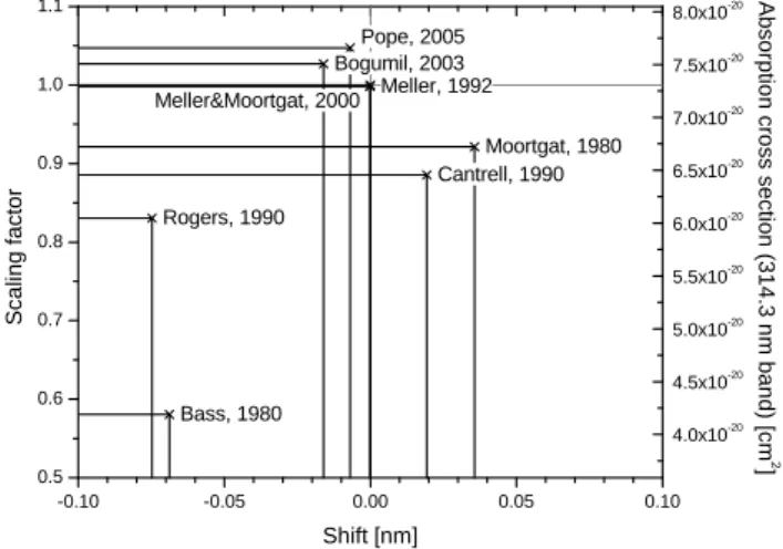
HONO were retrieved by simultaneously fitting resolution-adjusted reference spectra using the combined linear-nonlinear least squares algorithm (e.g. Stutz and Platt, 1996) of the MFC software (Gomer et al., 1995). Formaldehyde was identified by its four strong absorption bands in the UV between 310 and 337 nm, and calibrated using the literature cross-section by Meller and Moortgat (2000).
The stated uncertainty of the formaldehyde UV absorp-tion cross-secabsorp-tion is ±5% (Meller and Moortgat, 2000). Dif-ferences between the available CH2O cross-sections are
dis-cussed in Sect. 4.4. The systematic error of the DOAS spectrometer was determined to be <3% as described by Stutz (1996). The total systematic error of the CH2O
con-centrations, determined by the DOAS is therefore <6%. A mean detection limit of CH2O of 0.9 ppbv was determined
with an average time resolution of 137 s. 2.2 FTIR White system (CTH)
In Fourier-Transform Infra Red (FTIR) interferometry, the absorption of infrared light by various molecules is quanti-fied in the wavelength region between 2 and 15 µm. The open path FTIR White system was set up by CTH and ran semi-continuously over 28 days, between 22 July and 18 Au-gust. The system consisted of an infrared spectrometer cou-pled to an open path multi-reflection cell (White cell) with a base path of 25 m and a total path length of 1 km. The White cell was based on the retroreflector design outlined by Ritz et al. (1993) with minor modifications. An FTIR (BOMEM MB 100) computer-controlled spectrometer with a resolution of 1 cm−1 was employed. A 24 h dewar InSb detector was used covering the spectral region from 1800 to 3500 cm−1.
During the field campaign, the computer, FTIR spectrom-eter and field mirror of the FTIR White system were located inside the shipping container which also housed the DOAS system’s instrumentation. The objective mirrors of the FTIR White system were located on a tripod 25 m away from the field mirror. The spectra were analysed using the non-linear fitting software NLM (D. Griffith, personal communication), which is a further development of the MALT code (Griffith, 1996). In NLM, line parameters from the HITRAN compi-lation (Rothman, 1987) are convolved with appropriate in-strument parameters and subsequently least square fitted to the measured spectra to derive the average concentration of various molecules along the measurement path. Formalde-hyde was detected employing a characteristic doublet at 2779 and 2781.5 cm−1. During most of the campaign, 64 consec-utively recorded spectra were binned, thus yielding a mea-surement time resolution of 5 min. The meamea-surement pre-cision as obtained from the standard deviation of the CH2O
measurements is around 0.2 ppbv. The overall accuracy, as determined from the uncertainty of 5% in the spectroscopic data (Rothman et al., 1987), an offset which depends on the CH2O concentration and the precision, is specified to vary
from 27% for a measured mixing ratio of 2 ppbv to 6% for 15 ppbv.
2.3 Hantzsch fluorimetric monitors (IFU, PSI, BUW) This technique is based on sensitive wet chemical fluori-metric detection of CH2O, which requires the transfer of
formaldehyde from the gas phase into the liquid phase. This is accomplished quantitatively by stripping the CH2O from
the air in a stripping coil with a well defined exchange time between gas and liquid phase. The coil is kept at 10◦C to en-sure a quantitative sampling (>98%) of CH2O even at
pres-sures as low as 600 hPa. The gas flow is controlled by a mass flow controller with a precision of 1.5%, and a con-stant liquid flow is provided by a peristaltic pump. The de-tection of formaldehyde is based on the so-called “Hantzsch” reaction (Nash, 1953). It employs the fluorescence of
3,5-diacetyl-1,4-dihydrolutidine (DDL) at 510 nm, which is produced from the reaction of aqueous CH2O with a solution
containing 2,4-pentanedione (acetylacetone) and NH3
(am-monia). The excitation wavelength is 412 nm. Studies of interferences showed that the technique is very selective for formaldehyde, with the response for other molecules found in typically polluted air masses being several orders of mag-nitude lower. The technique is described in detail by Kelly and Fortune (1994).
This type of instrument was operated by three groups. The BUW used an Aero Laser CH2O analyser, model AL4001, a
commercially available instrument. The PSI monitor and the three IFU instruments were new versions of the AL4001, the AL4021, which is identical in the chemistry components, but with slight modifications mainly concerning the temperature stabilisation of the fluorimeter and the layout of the gas flow. All Hantzsch instruments were equipped with the same opti-cal filters. For the sake of brevity, the five instruments used in this intercomparison will be referred to as IFU1, IFU2, IFU3, PSI, and BUW. The time resolution of the instruments was ∼90 s with a delay time (0–90% of the final value af-ter a change in concentration) of about 4 min depending on the flow rate settings. The systems were calibrated once per day using liquid standards, which were prepared indepen-dently by each group. Zero adjustment was performed once per day (IFU), every six hours (PSI), and about six times per day (BUW), respectively. The Aero Laser instrument had a gas-phase detection limit of 150 pptv in the field. The ac-curacy and precision are indicated as ±15% or 150 pptv and
±10% or 150 pptv, respectively. The ozone cross sensitiv-ity is stated to be a positive signal of 200 pptv CH2O per
100 ppbv of ozone.
2.4 DNPH cartridges, HPLC/UV (JRC)
Carbonyl compounds were measured in two-hour periods during the day to determine their diurnal fluctuation in air.
Sampling was done according to the standard of the Eu-ropean Monitoring network, EMEP (Rembges et al., 1999). The air sample (flow 0.9–1.0 l/min) was drawn through an ozone scrubber (Waters Sep-Pak KI cartridges) before pass-ing into the 2,4-dinitrophenylhydrazine (DNPH) coated C18 cartridges (Waters Sep-Pak DNPH-cartridges). Airborne carbonyls are hereby collected as their non-volatile 2,4-dinitrophenylhydrazone derivatives.
The cartridges were eluted with 2.5 ml of acetonitrile in the laboratory, diluted with 2.5 ml of H2O and stored at 5◦C
un-til analysis. The samples were analysed by HPLC-UV (high performance liquid chromatography) with a temperature sta-bilised (20◦C) 30 cm×3.9 mm C18-coated silica gel (4 µm) column (NOVO-PAK) run in the gradient mode (0.9 ml/min). Detection and quantification were carried out at 360 nm. The employed eluents were H2O (A-eluent) and acetonitrile
(B-eluent). The gradient was programmed from 50% B to 90%
B in 42 min. The detection limit for this method was in the range of 5–20 ng formaldehyde (S/N=3).
A possible interference may be caused by the coelution of hydrazones of target compounds with hydrazones of other aldehydes and ketones. However, for the formaldehyde-hydrazone no interference has been reported to date. Due to high humidity clogging the sample cartridges during the night and early morning, the automatic sampling system was not used during night time and both the first and the last sam-ples were taken without ozone scrubber. Positive interference in the form of a number of extraneous peaks in the HPLC-UV chromatograms has been reported for C18 DNPH-cartridges, when used at high atmospheric ozone concentrations without ozone scrubber (Vairavamurthy et al., 1992). In the present study, sampling without ozone scrubber was only carried out at low ozone concentrations. Thus, positive interference is unlikely. Moreover, no extraneous peaks were monitored. However, as in all kinds of chromatographic analysis, coelu-tion of unknowns with the target analytes cannot be excluded. In previous studies of ambient air from this area, we have used the DNPH technique at low ozone concentrations with-out ozone scrubber and have been able to rule with-out interfer-ence from potential coelutants by analysis of the DNPH ex-tracts not only by HPLC-UV but also with HPLC coupled to atmospheric pressure mass spectrometry (Duane et al., 2002).
Blank samples were taken on a daily basis by exposing DNPH cartridges to open air without sample flow. The formaldehyde blank levels were all below 2 nmol/cartridge. For an air volume of 120 l this leads to a detection limit of 0.5 ppbv.
3 Description of the campaign
The intercomparison measurements were conducted in Bresso (northern Italy) between 23 July and 31 July 2002 as a part of the FORMAT-I campaign. The principal goal of the European project FORMAT “Formaldehyde as a tracer of photooxidation in the troposphere” was to obtain a better knowledge of the regional distribution of formaldehyde and its temporal behaviour in interaction with other major pho-tochemical constituents. This can lead to better prediction of smog episodes and to better quantification of emissions from traffic and biomass burning. The first week of the cam-paign was used to intercompare both similar instruments and different in-situ techniques, before the instruments were dis-tributed to the other sites within the Po Basin for the remain-der of the campaign. Three sites, upwind, urban and down-wind of Milan, were chosen along a south to north axis deter-mined by the prevailing daytime wind direction. Bresso was the site representative for urban conditions. Measurements of photooxidants at this site had already been conducted in the LOOP/PIPAPO field experiment 1998 (e.g. Neftel et al., 2002).
((a) b)
(a) (b)
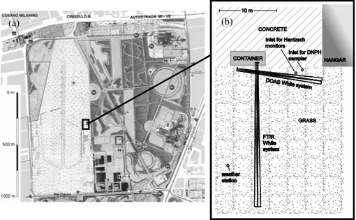
Fig. 1. (a) Surrounding area of the site at Bresso (MI), airfield and Parco Nord. (b) The setup of the instruments is shown on the right hand
side.
Bresso (at 45◦32.40N, 9◦12.10E, 146 m a.m.s.l.) is
situ-ated on the northern outskirts of Milan, 5 km north of the city centre, where vehicular and industrial emissions of CH2O
can mix with photochemically produced formaldehyde from anthropogenic and biogenic hydrocarbon emissions, so that both primary and secondary sources of CH2O are of
impor-tance. Possible sources for biogenic hydrocarbons are nearby local parks.
3.1 The measurement site
The measurement site was located on the premises of a small airfield (see Fig. 1a). The adjacent ∼1.2 km2in the west were grass-covered. The closest sources for road traffic emissions were a busy street 550 m to the west (Viale A. Grandi, with an adjacent residential area) and a major motorway (A4 Torino – Venezia) 1000 m to the north. The Parco Nord, a ∼2.2 km2 green recreation area was located directly to the east. Several hundred metres farther to the east, the Viale Fulvio Testi, a main road with high traffic density, leads to the city centre. There are no known emission sources for CH2O in the direct
surroundings of the site, apart from two lorry events, which are mentioned below.
The physical arrangement of the instruments is sketched in Fig. 1b. A shipping container housed the main mirror of the FTIR and the spectrographs of both White systems. The DOAS main mirror was placed in front of the container. The light paths of the White systems were set up approximately 1.5 m above the ground with a crossing alignment. For the comparison with the spectroscopic techniques, the sampling ports of the Hantzsch monitors and the DNPH-sampler were mounted close to the intersecting pathways of both multi-reflection systems in a height of about 1.2 m above ground
and at a distance of a few metres from each other. Thus, sampling of the same air mass can be implied. The Hantzsch monitors were sampling from a 10 m common PFA inlet line with 4 mm inner diameter, which lead to a hangar where the Hantzsch instruments were operated. The sampling altitude was 1.2 m above ground. The inlet line was protected from apparent aerosols by a nuclepore inline filter (47 mm diame-ter, 0.5 µm pore size), which was replaced once per day.
In addition to formaldehyde, ozone (up to 85 ppbv), nitro-gen dioxide (up to 40 ppbv), sulphur dioxide, nitrous acid, carbon monoxide, nitric oxide, other carbonyls and meteoro-logical parameters were measured simultaneously at the site throughout the campaign.
3.2 Atmospheric conditions during the intercomparison During the first half of the intercomparison period, the syn-optic situation over Central Europe was affected by a zonal flow in the 500 hPa level. An upper-tropospheric ridge which developed after 27 July and an associated surface high pres-sure area extending over southern and central Europe gov-erned the second half of the intercomparison week, lead-ing to fair weather conditions. Its impact was superseded by a trough evolving over Ireland which introduced a low-pressure episode after 31 July. A cyclonic flow pattern devel-oped steering low pressure systems on a track passing over Northern Italy.
Measurements of the standard meteorological parameters were performed continuously at the intercomparison site. The temperature during the intercomparison week varied be-tween 17 and 32◦C with strong diurnal variations. The global radiation reached 800 W/m2every day. The conditions were appropriate for moderate photooxidant production. Under
these conditions, daytime ozone mixing ratios of up to 85 ppbv were measured at the site. The ozone levels dropped to zero due to titration with NO from local emissions and deposition during the night. The relative humidity reached 75–100% during several nights and was typically 50–60% during the day, with an average of 62% over the complete week. There were no rain events in the greater Milan area during the intercomparison week.
At night and during the early morning hours, the wind (measured at 2 m height) generally came from the north and wind speeds were low. Calm winds below 3.5 m/s with southerly components were observed during the day, begin-ning in the late morbegin-ning thus providing air from downtown Milan. This diurnal change of air flow in the Po Basin arises from a mesoscale circulation which is orographically induced by a heat low over the Alps, leading to a southern wind direction during daytime and a flow from north to south during the night.
4 Results
4.1 Intercomparison of ambient measurements
After the campaign the final formaldehyde data of the indi-vidual groups was openly collected and compared. The tem-poral resolution of the data ranged from two to five minutes for the optical instruments and the Hantzsch monitors (these methods will hence be referred to as “continuous methods”), whereas the DNPH method required two hours for each sam-ple. Due to the different measurement intervals of the var-ious instruments, each of the continuous instruments’ data sets was integrated and 30 min averages were calculated on a common time scale. When compared to the DNPH results, the data was integrated over two hours.
Figure 2 presents the formaldehyde mixing ratio time se-ries as measured (a) by the Hantzsch instruments, and (b) by the optical methods. Because large differences between DOAS and Hantzsch results were found (e.g. Grossmann et al., 2003), (c) shows a direct comparison between DOAS and BUW Hantzsch results. This Hantzsch monitor was operat-ing almost continuously. The time series of two-hour inte-grated values for each instrument is shown in (d), where the horizontal bars denote the CH2O levels and the duration of
the DNPH measurement periods.
Ambient mixing ratios between 1 and 13 ppbv (for the 30 min averages) were detected by all instruments, and the temporal variation was generally in good agreement. How-ever, the observations obtained from the IFU1 instrument are systematically higher than those from all other instruments until 28 July. After that date, IFU1 measured considerably lower concentrations than the other instruments. On 25 and 26 July, a diverging temporal behaviour of IFU2 was ob-served when compared to all other instruments (Fig. 2a). Af-ter 26 July, IFU2 levels are in good agreement with the other
Hantzsch levels. The accordance between the Hantzsch mon-itors IFU3, PSI and BUW was notably good. However, a slight offset between the results of IFU3 and PSI compared to those of BUW is discernible. The overall agreement between the DOAS measurements and the BUW Hantzsch is good (Fig. 2c). Particularly large offsets between the two meth-ods, as reported in previous comparisons (see Sect. 1), were not detected. Occasionally occurring differences are likely due to local inhomogeneities caused by cars or lorries. For the six days of DNPH measurements during the intercom-parison week, the rough temporal variation of the formalde-hyde concentration during the day was well described by the two-hour integrated measurements (Fig. 2d). The observed concentration levels agree with those of most of the continu-ous instruments. The discrepancies mentioned for IFU1 and IFU2 are recognisable here as well.
During the intercomparison week the formaldehyde mix-ing ratios were comparatively low for an urban site, vary-ing between 1 and 6 ppbv most of the time. Typical CH2O mixing ratios around 10 ppbv were reported for the
LOOP/PIPAPO campaign 1998 at the same site in Bresso (e.g. Alicke et al., 2002). Five days of the present study ex-hibit a diurnal pattern with minimum values during night and higher levels during daytime, whereas three consecutive days feature no pronounced diurnal variation and levels of around 4 ppbv. Two events of particularly high formaldehyde con-centration occurred on 24 July and 30 July. The first event was caused by lorries usually stored in the hangar nearby. During this event, however, they were parked within 100 m of the measurement site with their engines running idle. This incident gave rise to an experiment conducted on 30 July, when the lorries were placed close to the instruments with the diesel engines running. The rapid increase of CH2O, CO
and HONO within a few minutes indicates a distinct exhaust-gas plume and most probably an inhomogeneous formalde-hyde distribution within the probed air mass. Thus, the time series used for the intercomparison do not contain the data points from these two incidents. In the evening of 29 July, a change in the sampling line setup was performed. The in-lets of the Hantzsch instruments IFU1, BUW, and IFU2 were mounted at different height levels to measure possible verti-cal differences in the formaldehyde distribution. Therefore, the Hantzsch instruments were no longer sampling identical air masses, and these data points are not included in the in-tercomparison either.
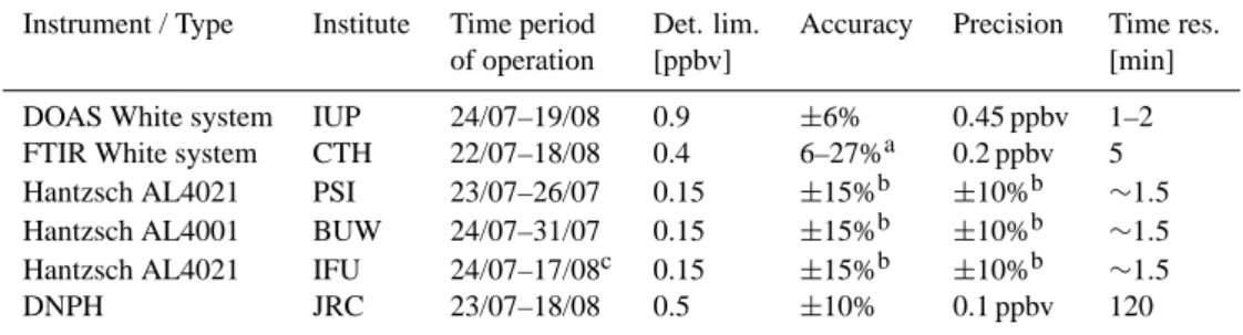
The data for the ambient measurements was compared by pairing sets of data for all combinations of instruments for which simultaneous measurements were taken. Linear regressions were calculated for each pair of instruments in order to compare slopes, intercepts, and correlation coeffi-cients. Since both data sets in the regression are subject to error, an ordinary least squares regression is inappropri-ate. Because only the vertical distances of the data points to the regression line (only y direction) are minimised, the true slope of the regression line is underestimated (Riggs et al.,
14 12 10 8 6 4 2 0 C H2 O [ p p b v] 23.7.02 24.7.02 25.7.02 26.7.02 27.7.02 28.7.02 29.7.02 30.7.02 31.7.02 1.8.02 B res s o Date [C E S T ] (a) Hantzs ch 1 'S N-1', IF U Hantzs ch 2 'S N11', IF U Hantzs ch 3 'S N28', IF U Hantzs ch, B UW Hantzs ch, P S I 14 12 10 8 6 4 2 0 C H2 O [ p p b v] 23.7.02 24.7.02 25.7.02 26.7.02 27.7.02 28.7.02 29.7.02 30.7.02 31.7.02 1.8.02 B res s o Date [C E S T ] F T IR W hite s ys tem, C T H DOAS W hite s ys tem, IUP (b) 14 12 10 8 6 4 2 0 C H2 O [ p p b v] 23.7.02 24.7.02 25.7.02 26.7.02 27.7.02 28.7.02 29.7.02 30.7.02 31.7.02 1.8.02 B res s o Date [C E S T ]
DOAS W hite s ys tem, IUP Hantzs ch, B UW (c) 10 8 6 4 2 0 C H2 O , 2 h a vg [ p p b v] 23.7.02 24.7.02 25.7.02 26.7.02 27.7.02 28.7.02 29.7.02 30.7.02 31.7.02 1.8.02 B res s o Date [C E S T ] (d) DNP H, J R C
DOAS W hite s ys tem, IUP F T IR W hite s ys tem, C T H Hantzs ch 1, IF U Hantzs ch 2, IF U Hantzs ch 3, IF U Hantzs ch, P S I Hantzs ch, B UW
Fig. 2. (a–c) Formaldehyde time series as half hourly averages (ticks at 00:00 Central European Summer Time) at Bresso during the
inter-comparison week as measured (a) by the five Hantzsch monitors, and (b) by the optical techniques FTIR and DOAS. (c) Direct inter-comparison of the DOAS (yellow triangles) and BUW Hantzsch monitor (blue rhombs) results. Note that the two peaks occurring on 30 July can be attributed to a local lorry emission source initiated by the experimentalists. Those points were omitted for the intercomparison. (d) Formalde-hyde measurements by the continuous instruments DOAS, FTIR and Hantzsch (as two hour averages) and DNPH (samples of two hours). The length of the horizontal lines corresponds to the duration of the DNPH measurement periods.
1978). Thus, the regressions were calculated using a method which is often called orthogonal regression. This method minimises the distance in both directions (both y and x di-rection). Individual errors of the data points are accounted for by a weighted line fit described in Press et al. (1992). Scatter plots for almost all pairs of continuous instruments are shown in Fig. 3a–r. The statistical data for all combina-tions are depicted in the plots and summarised in Table 2. After a modification in the instrument on 28 July, IFU1 mea-sured lower values. The two time periods before and after
this modification are considered separately in the following regression analysis, and the markers for the second period are displayed as stars in Fig. 3. After a change in the system on 26 July, the agreement between IFU2 and the other instru-ments is good. Only the measureinstru-ments taken after 26 July are considered reliable. Thus, the regression results of IFU2 shown in Table 2 exclude the first two days of operation.
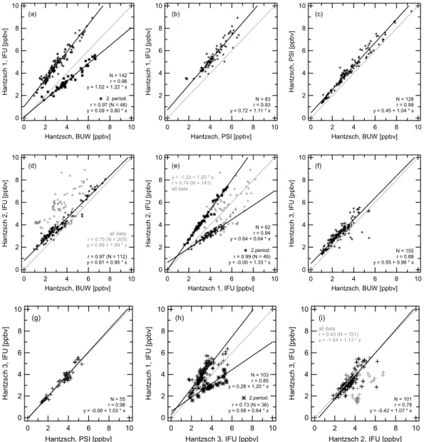
10 8 6 4 2 0 H an tz sc h 1, IF U [p pb v] 10 8 6 4 2 0 Hantzsch, BUW [ppbv] (a) N = 142 r = 0.96 y = 1.02 + 1.22 * x 2. period: r = 0.97 (N = 48) y = 0.09 + 0.80 * x 10 8 6 4 2 0 H an tz sc h 1, IF U [p pb v] 10 8 6 4 2 0 Hantzsch, PSI [ppbv] (b) N = 83 r = 0.93 y = 0.72 + 1.11 * x 10 8 6 4 2 0 H an tz sc h, P SI [p pb v] 10 8 6 4 2 0 Hantzsch, BUW [ppbv] (c) N = 128 r = 0.99 y = 0.45 + 1.04 * x 10 8 6 4 2 0 H an tz sc h 2, IF U [p pb v] 10 8 6 4 2 0 Hantzsch, BUW [ppbv] (d) all data: r = 0.75 (N = 205) y = 0.99 + 1.09 * x r = 0.97 (N = 112) y = 0.81 + 0.95 * x 10 8 6 4 2 0 H an tz sc h 2, IF U [p pb v] 10 8 6 4 2 0 Hantzsch 1, IFU [ppbv] (e) N = 62 r = 0.94 y = 0.64 + 0.64 * x 2.period: r = 0.99 (N = 49) y = -0.00 + 1.33 * x y = -1.33 + 1.20 * x r = 0.74 (N = 141) all data 10 8 6 4 2 0 H an tz sc h 3, IF U [p pb v] 10 8 6 4 2 0 Hantzsch, BUW [ppbv] (f) N = 155 r = 0.88 y = 0.55 + 0.98 * x 10 8 6 4 2 0 H an tz sc h 3, IF U [p pb v] 10 8 6 4 2 0 Hantzsch, PSI [ppbv] (g) N = 55 r = 0.98 y = -0.08 + 1.03 * x 10 8 6 4 2 0 H an tz sc h 1, IF U [p pb v] 10 8 6 4 2 0 Hantzsch 3, IFU [ppbv] (h) N = 103 r = 0.85 y = 0.28 + 1.20 * x 2.period: r = 0.73 (N = 38) y = 0.59 + 0.64 * x 10 8 6 4 2 0 H an tz sc h 3, IF U [p pb v] 10 8 6 4 2 0 Hantzsch 2, IFU [ppbv] (i) N = 101 r = 0.78 y = -0.42 + 1.07 * x all data: r = 0.45 (N = 151) y = -1.04 + 1.13 * x
Fig. 3. (a–r) Scatter plots for most pairs of the seven continuously measuring instruments taking part in the intercomparison. The CH2O
mixing ratios are plotted versus one another for matched times of measurements, and linear regressions were calculated. The solid lines drawn through the data correspond to the weighted orthogonal least squares fit to the data (black) (York, 1966), and the one to one correspondence line (grey), respectively. For the two periods of IFU1 measurements (before and after 28 July 12:00) individual regressions were calculated. Additional grey markers indicate questionable IFU2 data points before 26 July. Regression parameters for the overall data sets and subsets are given in the plots.
4.1.1 Agreement among the Hantzsch instruments (a)–(i)
The Hantzsch instruments PSI, BUW, IFU1, and IFU3 cor-relate very well. The correlation coefficients exceed r=0.9 for most combinations (Fig. 3a–g, Table 2). The highest degree of correlation was found between the two Hantzsch instruments PSI and BUW with a correlation coefficient of
r=0.99 for the three days of simultaneous measurements. The slope of the regression line is near unity (b=1.04), but there is a positive offset of 0.46 ppbv for PSI, significant at the 95% level. A similar result was found for IFU3 with a
slope of b=0.98 and an offset of 0.55 ppbv when compared to BUW. IFU3 and PSI agree with a high degree of corre-lation (r=0.98). The linear regression reveals a slope not significantly different from unity and no offset. However, IFU1 measured systematically higher values for the first pe-riod, when compared to IFU3, PSI and BUW, which is ev-ident in the slopes of the regression lines: They are signif-icantly steeper than one and show non-zero intercepts. For the second period, IFU1 measures distinctly lower concen-trations than all other instruments. This becomes apparent by the second regression line.
10 8 6 4 2 0 FT IR W hi te s ys te m , C TH [p pb v] 10 8 6 4 2 0 Hantzsch, BUW [ppbv] (j) N = 105 r = 0.82 y = 0.63 + 0.90 * x 10 8 6 4 2 0 FT IR W hi te s ys te m , C TH [p pb v] 10 8 6 4 2 0 Hantzsch, PSI [ppbv] (k) N = 77 r = 0.72 y = 0.25 + 0.88 * x 10 8 6 4 2 0 FT IR W hi te s ys te m , C TH [p pb v] 10 8 6 4 2 0 Hantzsch 1, IFU [ppbv] (l) 2.period: r = 0.92 (N = 18) y = -5.87 + 2.51 * x y = -0.19 + 0.79 * x r = 0.65 (N = 73) 10 8 6 4 2 0 FT IR W hi te s ys te m , C TH [p pb v] 10 8 6 4 2 0 Hantzsch 3, IFU [ppbv] (m) N = 54 r = 0.47 y = 0.60 + 0.77 * x 10 8 6 4 2 0 D O AS W hi te s ys te m , I U P [p pb v] 10 8 6 4 2 0 Hantzsch, BUW [ppbv] (n) N = 133 r = 0.90 y = 0.39 + 0.96 * x 10 8 6 4 2 0 D O AS W hi te s ys te m , I U P [p pb v] 10 8 6 4 2 0 Hantzsch, PSI [ppbv] (o) N = 57 r = 0.81 y = -0.15 + 0.92 * x 10 8 6 4 2 0 D O AS W hi te s ys te m , I U P [p pb v] 10 8 6 4 2 0 Hantzsch 1, IFU [ppbv] (p) 2.period: r = 0.82 (N = 36) y = 0.71 + 1.06 * x y = -0.93 + 0.90 * x r = 0.71 (N = 79) 10 8 6 4 2 0 D O AS W hi te s ys te m , I U P [p pb v] 10 8 6 4 2 0 Hantzsch 3, IFU [ppbv] (q) N = 100 r = 0.70 y = -0.02 + 0.98 * x 20 18 16 14 12 10 8 6 4 2 0 D O AS W hi te s ys te m , I U P [p pb v] 20 18 16 14 12 10 8 6 4 2 0
FTIR White system, CTH [ppbv] (r)
r = 0.81 (N = 90) y = 0.40 + 0.92 * x
with lorry (10 min): r = 0.89 (N = 213) y = 0.10 + 1.03 * x
Fig. 3. Continued.
The correlation and regression analysis including IFU2 results shows little agreement with correlation coefficients between 0.45 and 0.75 if one considers the complete IFU2 data set (grey markers). The data points are highly scattered around the regression lines (figures not shown here). The scattering for IFU2 can partly be attributed to the diverging results as a consequence of malfunction of the system on 25 and 26 July (Fig. 2a). If one considers only the reliable IFU2 data points after 26 July, there are no mutual points with PSI, but the comparison with BUW yields r=0.97, b=0.95,
a=0.81. IFU1 and IFU2 agreed considerably better after 26 July (r=0.94) than for the entire data set, but with a slope of only b=0.64 (a=0.64), which to some degree matches the previously observed positive bias of IFU1.
Possible reasons for the disagreement among these five nearly identical instruments are discussed in Sect. 4.3.
4.1.2 Agreement between spectroscopic and Hantzsch techniques (j)–(q)
The FTIR measurements compare quite well with the BUW Hantzsch data, with a slope close to unity (b=0.90, a=0.63). Similarly, a regression line with no significant deviation from the one-to-one line was found for FTIR versus PSI. As a smaller number of data points was available, the degree of correlation is somewhat lower (Fig. 3k). The correlation co-efficient between FTIR and IFU1 data for the time span un-til 28 July is lower (r=0.65). There is a significant deviation from the 1:1 line (b=0.79), with IFU1 showing the larger val-ues. After 28 July IFU1 measures significantly lower concen-trations than the FTIR. A good agreement was found between FTIR and IFU2 (values after 26 July) with a slope of b=0.97 (r=0.90), whereas the employment of the complete data set
Table 2. Results of the orthogonal regression analysis (York, 1966) between the continuous instruments (see also Fig. 3). [CH2O]y=a+b [CH2O]x, where y and x are the corresponding in-struments, and a and b are the intercept and slope of the regression line, respectively with 95% confidence intervals. N is the number of data points included in the regression, and r is Pearson’s corre-lation coefficient. The first column indicates the corresponding plot in Fig. 3 (for some regressions no plot is shown).
Fig. y x a[ppbv] b r N a) IFU 1∗ BUW 1.02±0.17 1.22±0.05 0.96 142 b) IFU 1 PSI 0.72±0.40 1.11±0.09 0.93 83 c) PSI BUW 0.46±0.12 1.04±0.03 0.99 128 d) IFU 2∗ BUW 0.81±0.15 0.95±0.04 0.97 112 -) IFU 2 PSI 1.49±0.65 0.96±0.16 0.58 100 e) IFU 2∗ IFU 1 0.64±0.22 0.64±0.06 0.94 62 f) IFU 3 BUW 0.55±0.21 0.98±0.07 0.88 155 g) IFU 3 PSI −0.08±0.21 1.03±0.06 0.98 55 h) IFU 1∗ IFU 3 0.28±0.39 1.20±0.12 0.85 103 i) IFU 3 IFU 2∗ −0.42±0.47 1.07±0.13 0.78 101 j) FTIR BUW 0.63±0.40 0.90±0.09 0.82 105 k) FTIR PSI 0.25±0.74 0.88±0.14 0.72 77 l) FTIR IFU 1∗ −0.19±0.73 0.79±0.14 0.65 73 -) FTIR IFU 2∗ −0.22±0.71 0.97±0.15 0.90 35 m) FTIR IFU 3 0.60±0.62 0.77±0.16 0.47 54 n) DOAS BUW 0.39±0.27 0.96±0.08 0.90 132 o) DOAS PSI −0.15±0.56 0.92±0.15 0.81 57 p) DOAS IFU 1∗ −0.93±0.84 0.90±0.18 0.71 79 -) DOAS IFU 2∗ −0.07±0.49 0.93±0.11 0.93 69 q) DOAS IFU 3 −0.02±0.48 0.98±0.15 0.70 100 r) DOAS FTIR 0.40±0.39 0.92±0.09 0.81 90
∗Note that the regression results given for the IFU2 instrument were
calculated omitting the data of 25 and 26 July, and the regression results for IFU1 exclude data after 28 July, 09:15 CEST.
shows strong scattering. No coherence is recognizable be-tween FTIR and IFU3, where only 54 mutual data points are available. The observed concentration range is very small here.
A large amount of mutual data points was obtained for the pair DOAS and BUW, where a good correlation (r=0.90) is found. The slope of the regression line is not significantly different from unity (b=0.96). There was also good agree-ment between DOAS and PSI (r=0.81, b=0.92). The 1:1 line is enclosed within the 95% confidence interval of the regression slope and there is no significant offset. IFU1 first measured considerably higher values than the DOAS (b=0.90, a=−0.93). The result for the second period is shown by the second regression line in Fig. 3p. For values af-ter 26 July, the agreement between DOAS and IFU2 is good (r=0.93, b=0.93, no significant offset). However, including the complete IFU2 data set reveals less agreement. The re-gression between DOAS and IFU3 displays a slope not sig-nificantly different from unity and no significant offset.
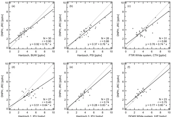
Table 3. Linear orthogonal regressions (York, 1966) for the
correla-tions between DNPH and the continuous methods (see also Fig. 4). The definition of parameters is specified in Table 2.
Fig. y x a[ppbv] b r N a) DNPH BUW 0.92±0.45 0.76±0.12 0.90 30 b) DNPH PSI 0.37±0.75 0.76±0.16 0.86 26 c) DNPH FTIR 0.76±0.87 0.74±0.20 0.66 31 d) DNPH IFU 1 0.51±1.08 0.64±0.23 0.40 27 -) DNPH IFU 2∗ −0.23±1.71 0.97±0.48 0.59 13 e) DNPH IFU 3 0.28±0.88 0.83±0.24 0.74 23 f) DNPH DOAS 0.77±0.81 0.80±0.23 0.75 23
4.1.3 Agreement among spectroscopic techniques (r) The FTIR measured predominantly during daylight hours, whereas the DOAS system was generally also operated at night (Fig. 2b). Altogether, there are 90 mutual points be-tween the two White systems (30 min averages) during the intercomparison week. The correlation is moderate with
r=0.81. At the 95% confidence level the regression slope (b=0.92) is not significantly different from unity.
Both instruments detect the average concentrations along the respective light paths. During the intensive lorry experi-ment, the lorries were located upwind of the air volume sur-veyed by both White systems. A comparison was performed using 10 min averages, due to the temporal limitation of the experiment to two events of 30 min each. Maximum values around 19 ppbv (10 min average) were measured by both in-struments during the lorry experiment and a correlation of
r=0.89 and a slope of b=1.03 were found, thus nearly yield-ing a one-to-one correspondence. The dashed line in Fig. 3r is the regression line to the ten minute data including the lorry experiment (grey markers).
4.1.4 Agreement between continuous instruments and DNPH
The DNPH samples were taken every two hours during day-time. Therefore two hour averages of the continuous instru-ments were compared to the integrated results obtained from the cartridges. As mentioned before, the data containing the lorry plumes was omitted in the calculations. The results are presented in scatter plots in Fig. 4a–f. The statistical parameters are summarised in Table 3. For all cases, the regression slopes are below unity, however for IFU2, IFU3 and DOAS unity is included within the 95% confidence in-terval. The regression analysis for DNPH versus Hantzsch BUW and PSI revealed slopes of b=0.76 and correlation co-efficients of around r=0.90. The instruments IFU1, IFU2, IFU3 attained correlation coefficients of r=0.40, 0.59, 0.74 (note the different measurement intervals; IFU2 values af-ter 26 July) with systematically higher values for IFU1 than
10 8 6 4 2 0 D N PH , J R C [p pb v] 10 8 6 4 2 0 Hantzsch, BUW [ppbv] (a) N = 30 r = 0.90 y = 0.92 + 0.76 * x 10 8 6 4 2 0 D N PH , J R C [p pb v] 10 8 6 4 2 0 Hantzsch, PSI [ppbv] (b) N = 26 r = 0.86 y = 0.37 + 0.76 * x 10 8 6 4 2 0 D N PH , J R C [p pb v] 10 8 6 4 2 0
FTIR White system, CTH [ppbv] (c) N = 31 r = 0.66 y = 0.76 + 0.74 * x 10 8 6 4 2 0 D N PH , J R C [p pb v] 10 8 6 4 2 0 Hantzsch 1, IFU [ppbv] (d) N = 27 r = 0.40 y = 0.51 + 0.64 * x 10 8 6 4 2 0 D N PH , J R C [p pb v] 10 8 6 4 2 0 Hantzsch 3, IFU [ppbv] (e) N = 23 r = 0.74 y = 0.28 + 0.83 * x 10 8 6 4 2 0 D N PH , J R C [p pb v] 10 8 6 4 2 0
DOAS White system, IUP [ppbv] (f)
N = 23 r = 0.75 y = 0.77 + 0.80 * x
Fig. 4. Regressions of the DNPH cartridge results from the intercomparison week plotted versus those from continuous techniques for
concordant two hour time spans. The solid black line drawn through the data is the orthogonal least squares fit to the data (York, 1966). The grey line represents the one to one correspondence.
for the DNPH. The slopes of IFU1, IFU2, IFU3 are b=0.64, 0.97, 0.83. Plotting the DNPH data versus the FTIR data also reveals a regression slope lower than unity (b=0.74) and an intercept not significantly different from zero (correlation coefficient r=0.66).
The mixing ratios measured by DNPH, Hantzsch, DOAS, and FTIR techniques correspond moderately well to each other on the two hour time scale. However, short term varia-tions cannot be resolved. In summary, the DNPH results are slightly lower than those measured by the continuous instru-ments for up to 30 common data points in the concentration range from 1 to 8 ppbv.
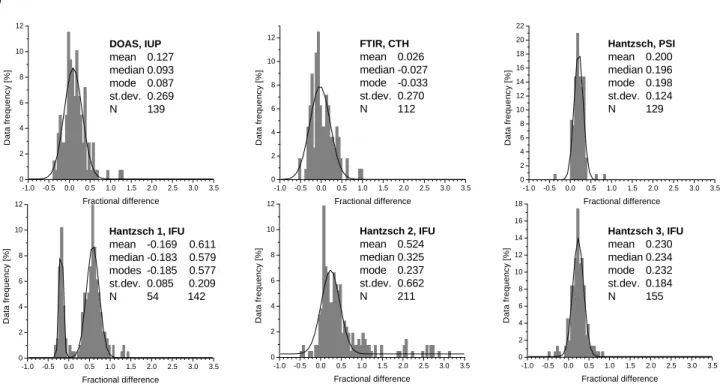
4.2 Fractional differences
The agreement between measurements of the continuous instruments and a reference instrument is summarised in histograms of the fractional differences δ=([CH2O]instr
-[CH2O]ref)/[CH2O]ref. For the comparison among the
con-tinuous instruments, the BUW Hantzsch was chosen as a ref-erence because it was almost continuously operating over the entire intercomparison period. The results are depicted in Fig. 5a for the overall data sets. Figure 5b shows the resulting fractional differences for the two-hour integrated measure-ments of all instrumeasure-ments, using the DNPH data as reference.
The plots show the histograms of the data (shaded bars) and fitted Gaussian functions (black curve). The respective statistical information is given in the legend of each plot. The fact that the average, median, and mode (i.e., the most prob-able fractional difference) of the PSI, IFU1, and IFU3 dis-tributions are similarly positioned suggests symmetry in the distributions and therefore mostly random differences. The PSI histogram has a narrow distribution with a standard de-viation of σ =0.12. The DOAS, FTIR, IFU1, IFU2, and IFU3 histograms show σ of 0.27, 0.27, 0.21, 0.66 and 0.18, re-spectively. The IFU2 histogram has a slightly skew distri-bution which is due to the erroneous results from 25 and 26 July. After eliminating those outliers, the IFU2 histogram shows an almost symmetrical δ-distribution. In this case, the average, median, and mode are nearly collocated (aver-age=0.23, median=0.19, mode=0.21) and the standard devi-ation is decreased to 0.24. The distributions for the spectro-scopic techniques DOAS and FTIR are wider than those for most of the Hantzsch instruments. Most instruments show a positive bias with respect to the reference BUW Hantzsch instrument. The relative difference between the DOAS and the BUW Hantzsch is +9%. On average, 3% lower val-ues were found for the FTIR than for the BUW. The PSI, IFU1, IFU2 and IFU3 values were approximately 20, 58, 21 and 23% higher than the BUW results, respectively. After the instrumental modification of IFU1, the results were 19%
(a) - 1 . 0 - 0 . 5 0 . 0 0 . 5 1 . 0 1 . 5 2 . 0 2 . 5 3 . 0 3 . 5 0 2 4 6 8 1 0 1 2 D a ta f re q u e n c y [ % ] F r a c t i o n a l d i f f e r e n c e H a n t z s c h 1 , I F U m e a n - 0 . 1 6 9 3 7 0 . 6 1 1 0 6 m e d i a n - 0 . 1 8 2 7 4 0 . 5 7 8 8 6 m o d e s - 0 . 1 8 5 5 2 0 . 5 7 7 4 4 s t . d e v . 0 . 0 8 4 9 9 0 . 2 0 9 5 0 N 5 4 1 4 2 - 1 . 0 - 0 . 5 0 . 0 0 . 5 1 . 0 1 . 5 2 . 0 2 . 5 3 . 0 3 . 5 0 2 4 6 8 1 0 1 2 1 4 1 6 1 8 2 0 2 2 D a ta f re q u e n c y [ % ] F r a c t i o n a l d i f f e r e n c e H a n t z s c h , P S I m e a n 0 . 2 0 0 5 5 m e d i a n 0 . 1 9 5 6 2 m o d e 0 . 1 9 8 5 3 s t . d e v . 0 . 1 2 4 0 0 N 1 2 9 - 1 . 0 - 0 . 5 0 . 0 0 . 5 1 . 0 1 . 5 2 . 0 2 . 5 3 . 0 3 . 5 0 2 4 6 8 1 0 1 2 D a ta f re q u e n c y [ % ] F r a c t i o n a l d i f f e r e n c e F T I R , C T H m e a n 0 . 0 2 5 9 8 m e d i a n - 0 . 0 2 6 6 6 m o d e - 0 . 0 3 3 1 1 s t . d e v . 0 . 2 6 9 6 9 N 1 1 2 - 1 . 0 - 0 . 5 0 . 0 0 . 5 1 . 0 1 . 5 2 . 0 2 . 5 3 . 0 3 . 5 0 2 4 6 8 1 0 1 2 D a ta f re q u e n c y [ % ] F r a c t i o n a l d i f f e r e n c e D O A S , I U P m e a n 0 . 1 2 7 2 4 m e d i a n 0 . 0 9 3 3 m o d e 0 . 0 8 7 3 4 s t . d e v . 0 . 2 6 9 2 8 N 1 3 9 - 1 . 0 - 0 . 5 0 . 0 0 . 5 1 . 0 1 . 5 2 . 0 2 . 5 3 . 0 3 . 5 0 2 4 6 8 1 0 1 2 D a ta f re q u e n c y [ % ] F r a c t i o n a l d i f f e r e n c e H a n t z s c h 2 , I F U m e a n 0 . 5 2 4 1 8 m e d i a n 0 . 3 2 4 6 1 m o d e 0 . 2 3 6 8 8 s t . d e v . 0 . 6 6 1 6 1 N 2 1 1 - 1 . 0 - 0 . 5 0 . 0 0 . 5 1 . 0 1 . 5 2 . 0 2 . 5 3 . 0 3 . 5 0 2 4 6 8 1 0 1 2 1 4 1 6 1 8 D a ta f re q u e n c y [ % ] F r a c t i o n a l d i f f e r e n c e H a n t z s c h 3 , I F U m e a n 0 . 2 2 9 8 m e d i a n 0 . 2 3 4 1 2 m o d e 0. 2 3 2 5 1 s t . d e v . 0 . 1 8 4 2 3 N 1 5 5 D O A S , I U P m e a n 0 . 1 2 7 m e d i a n 0 . 0 9 3 m o d e 0 . 0 8 7 s t . d e v . 0 . 2 6 9 N 1 3 9 F T I R , C T H m e a n 0 . 0 2 6 m e d i a n - 0 . 0 2 7 m o d e - 0 . 0 3 3 s t . d e v . 0 . 2 7 0 N 1 1 2 H a n t z s c h , P S I m e a n 0 . 2 0 0 m e d i a n 0 . 1 9 6 m o d e 0 . 1 9 8 s t . d e v . 0 . 1 2 4 N 1 2 9 H a n t z s c h 3 , I F U m e a n 0 . 2 3 0 m e d i a n 0 . 2 3 4 m o d e 0 . 2 3 2 s t . d e v . 0 . 1 8 4 N 1 5 5 H a n t z s c h 2 , I F U m e a n 0 . 5 2 4 m e d i a n 0 . 3 2 5 m o d e 0 . 2 3 7 s t . d e v . 0 . 6 6 2 N 2 1 1 H a n t z s c h 1 , I F U m e a n - 0 . 1 6 9 0 . 6 1 1 m e d i a n - 0 . 1 8 3 0 . 5 7 9 m o d e s - 0 . 1 8 5 0 . 5 7 7 s t . d e v . 0 . 0 8 5 0 . 2 0 9 N 5 4 1 4 2
Fig. 5. Fractional difference histograms for each of the formaldehyde instruments calculated relative to a reference instrument. For the
comparison of (a) the continuously measuring techniques, the reference instrument is the BUW Hantzsch monitor, in (b) the reference instrument is the DNPH sampler. Each panel shows the frequency for the data falling into 0.05 fractional difference bins (normalised to the number of coincident data pairs). The legends show the statistics for the complete data sets.
smaller than those from BUW. In order to verify the rela-tive differences between the results of the seven instruments, fractional differences were also calculated using DOAS as a reference (Table 4, lower row). The previous result was con-firmed, with the Hantzsch measurements (except IFU1) be-ing within the ±11% range of the DOAS. DOAS and FTIR agree within 5%. This is also consistent with the uncertainty of the used cross-sections. The relative deviations obtained with the fractional differences are in line with the uncertain-ties expected from Table 2.
As the sample size is small for the fractional differences relative to DNPH (N=23–31, see Table 3), it was refrained from fitting Gaussians to the histograms (Fig. 5b). The dis-tributions for DOAS, FTIR, PSI and IFU3 are almost sym-metrical. The histogram for IFU2 is less symmetrical be-cause of several higher fractional differences be-caused by the instrumental problems during the first days. If these days are omitted, only two days of common data points are remaining. The data sets of DOAS, FTIR, PSI, IFU3, and BUW agreed with the DNPH results within ∼15%. For IFU1 and IFU2, the differences were larger. Mean and median coincide only in a few cases. Due to the small sample sizes of only 20– 30 data points, the statistical information should be regarded carefully in this part of the study.
4.3 Comparison of Hantzsch calibration standards
Formaldehyde solutions with a known concentration are re-quired in the calibration of the Hantzsch instruments. These solutions are produced by diluting a commercially available 37% CH2O-solution to a stock-solution of about 10−1 to
10−2mol/l, which is titrated regularly and is then further diluted to about 10−6mol/l for calibration (see also Aero Laser AL4001 HCHO analyser manual). Formaldehyde so-lutions with high concentrations contain a significant fraction of para-formaldehyde which interferes with the titration. Al-though the para-formaldehyde concentration is negligible in diluted solutions, a waiting time of at least 24 h between di-lution and titration is recommended to ensure the conversion of all para-formaldehyde. These diluted solutions are stable over years, with less than 0.2 percent deviation within one year.
The IFU 0.01 mol/l and PSI 0.05 mol/l diluted standards were both shown to be stable within less than a percent devi-ation over several years. The field standards were taken from these working standards, stored in cooled boxes and further diluted to concentrations of ∼10−6mol/l in the field for cal-ibration. At this level of dilution, the solution is no longer stable for more than one hour even when stored in a refriger-ator.
(b) - 1 . 0 - 0 . 5 0 . 0 0 . 5 1 . 0 1 . 5 2 . 0 2 . 5 3 . 0 0 2 4 6 8 1 0 1 2 D a ta f re q u e n c y [ % ] F r a c t i o n a l d i f f e r e n c e H a n t z s c h , P S I m e a n 0 . 1 9 0 5 2 m e d i a n 0 . 1 4 5 9 5 s t . d e v . 0 . 2 2 5 8 6 N 2 7 - 1 . 0 - 0 . 5 0 . 0 0 . 5 1 . 0 1 . 5 2 . 0 2 . 5 3 . 0 0 2 4 6 8 1 0 1 2 1 4 1 6 1 8 2 0 D a ta f re q u e n c y [ % ] F r a c t i o n a l d i f f e r e n c e H a n t z s c h , B U W m e a n - 0 . 0 4 1 4 3 m e d i a n - 0 . 0 9 0 0 0 s t . d e v . 0 . 1 9 3 6 1 N 3 1 - 1 . 0 - 0 . 5 0 . 0 0 . 5 1 . 0 1 . 5 2 . 0 2 . 5 3 . 0 0 2 4 6 8 1 0 1 2 1 4 1 6 D a ta f re q u e n c y [ % ] F r a c t i o n a l d i f f e r e n c e F T I R , C T H m e a n 0 . 0 8 2 5 8 m e d i a n 0 . 0 2 3 8 4 s t . d e v . 0 . 2 9 0 8 5 N 3 2 - 1 . 0 - 0 . 5 0 . 0 0 . 5 1 . 0 1 . 5 2 . 0 2 . 5 3 . 0 0 5 1 0 1 5 2 0 D a ta f re q u e n c y [ % ] F r a c t i o n a l d i f f e r e n c e D O A S , I U P m e a n - 0 . 0 3 1 0 6 m e d i a n - 0 . 0 7 3 3 3 s t . d e v . 0 . 1 6 6 5 6 N 2 3 - 1 . 0 - 0 . 5 0 . 0 0 . 5 1 . 0 1 . 5 2 . 0 2 . 5 3 . 0 0 2 4 6 8 1 0 1 2 1 4 1 6 1 8 2 0 2 2 D a ta f re q u e n c y [ % ] F r a c t i o n a l d i f f e r e n c e H a n t z s c h 3 , I F U m e a n 0 . 1 1 3 0 2 m e d i a n 0 . 0 2 8 4 6 s t . d e v . 0 . 1 9 6 9 9 N 2 3 - 1 . 0 - 0 . 5 0 . 0 0 . 5 1 . 0 1 . 5 2 . 0 2 . 5 3 . 0 0 2 4 6 8 1 0 1 2 1 4 1 6 D a ta f re q u e n c y [ % ] F r a c t i o n a l d i f f e r e n c e H a n t z s c h 2 , I F U m e a n 0 . 3 2 8 1 3 m e d i a n 0 . 1 7 9 5 0 s t . d e v . 0 . 4 1 3 7 1 N 2 7 - 1 . 0 - 0 . 5 0 . 0 0 . 5 1 . 0 1 . 5 2 . 0 2 . 5 3 . 0 0 5 1 0 1 5 2 0 2 5 D a ta f re q u e n c y [ % ] F r a c t i o n a l d i f f e r e n c e H a n t z s c h 1 , I F U m e a n 0 . 4 4 2 5 5 m e d i a n 0 . 3 3 0 6 6 s t . d e v . 0 . 3 2 3 7 0 N 2 4 D O A S , I U P m e a n - 0 . 0 3 1 m e d i a n - 0 . 0 7 3 s t . d e v . 0 . 1 6 6 N 2 3 F T I R , C T H m e a n 0 . 0 8 2 m e d i a n 0 . 0 2 4 s t . d e v . 0 . 2 9 1 N 3 2 H a n t z s c h , P S I m e a n 0 . 1 9 0 m e d i a n 0 . 1 4 6 s t . d e v . 0 . 2 2 6 N 2 7 H a n t z s c h 1 , I F U m e a n 0 . 4 4 2 m e d i a n 0 . 3 3 1 s t . d e v . 0 . 3 2 4 N 2 4 H a n t z s c h 2 , I F U m e a n 0 . 3 2 8 m e d i a n 0 . 1 7 9 s t . d e v . 0 . 4 1 4 N 2 7 H a n t z s c h 3 , I F U m e a n 0 . 1 1 3 m e d i a n 0 . 0 2 8 s t . d e v . 0 . 1 9 7 N 2 3 H a n t z s c h , B U W m e a n - 0 . 0 4 1 m e d i a n - 0 . 0 9 0 s t . d e v . 0 . 1 9 4 N 3 1 Fig. 5. Continued.
Table 4. Relative differences of the measurement results determined with reference to BUW Hantzsch (see also Fig. 5a) and to DOAS,
respectively.
DOAS FTIR PSI IFU 1 IFU 2 IFU 3 BUW
Relative to BUW Hantzsch +8.8% −3.3% +19.8% +57.7% +21.0% +23.2% – −18.5%
Relative to DOAS White cell – −5.1% +11.1% +41.3% +10.6% +7.2% −10.3%
−19.2
The liquid formaldehyde standards, which were used by IFU, PSI and BUW for the calibration of their Hantzsch in-struments, were independently prepared by each group.
At the beginning of the campaign (on 24 July), the stan-dard solutions (levels about 10−6mol/l) of the three groups were compared using one of the IFU instruments (SN28, in this study called ‘IFU3’). Each group prepared a solution of
∼10−6mol/l from the individual standards. The standards
by BUW and PSI agreed within 5% (PSI/BUW=1.05). How-ever, the results indicated a ∼+30% deviation of the calibra-tion standards of IFU when compared to the other groups. A 6% difference between the standard solutions of BUW and PSI was found on the same day using the PSI instrument (PSI/BUW=1.06).
After the first discrepancies were observed in the data, the working standards of IFU and PSI were again analysed in

![Fig. y x a [ppbv] b r N a) IFU 1 ∗ BUW 1.02 ± 0.17 1.22 ± 0.05 0.96 142 b) IFU 1 PSI 0.72 ± 0.40 1.11 ± 0.09 0.93 83 c) PSI BUW 0.46 ± 0.12 1.04 ± 0.03 0.99 128 d) IFU 2 ∗ BUW 0.81±0.15 0.95±0.04 0.97 112 -) IFU 2 PSI 1.49 ± 0.65 0.96 ± 0.16 0.58 100 e) IF](https://thumb-eu.123doks.com/thumbv2/123doknet/14774686.593092/13.892.76.427.246.627/fig-ppbv-ifu-buw-ifu-psi-psi-buw.webp)