HAL Id: tel-01922051
https://hal.inria.fr/tel-01922051
Submitted on 14 Nov 2018
HAL is a multi-disciplinary open access
archive for the deposit and dissemination of sci-entific research documents, whether they are pub-lished or not. The documents may come from teaching and research institutions in France or abroad, or from public or private research centers.
L’archive ouverte pluridisciplinaire HAL, est destinée au dépôt et à la diffusion de documents scientifiques de niveau recherche, publiés ou non, émanant des établissements d’enseignement et de recherche français ou étrangers, des laboratoires publics ou privés.
Observer design and output feedback stabilization of
time varying systems
Saeed Ahmed
To cite this version:
Saeed Ahmed. Observer design and output feedback stabilization of time varying systems. Automatic Control Engineering. Bilkent University, 2018. English. �tel-01922051�
OBSERVER DESIGN AND OUTPUT
FEEDBACK STABILIZATION OF TIME
VARYING SYSTEMS
a dissertation submitted to
the graduate school of engineering and science
of bilkent university
in partial fulfillment of the requirements for
the degree of
doctor of philosophy
in
electrical and electronics engineering
By
Saeed Ahmed
Observer Design and Output Feedback Stabilization of Time Varying Systems
By Saeed Ahmed July 2018
We certify that we have read this dissertation and that in our opinion it is fully adequate, in scope and in quality, as a dissertation for the degree of Doctor of Philosophy. Hitay ¨Ozbay(Advisor) Fr´ed´eric Mazenc(Co-Advisor) ¨ Omer Morg¨ul Yıldıray Yıldız Aykut Yıldız
No academic titles, only the name V Approved for the Graduate School of Engineering and Science:
Ezhan Kara¸san
ABSTRACT
OBSERVER DESIGN AND OUTPUT FEEDBACK
STABILIZATION OF TIME VARYING SYSTEMS
Saeed Ahmed
Ph.D. in Electrical and Electronics Engineering Advisor: Hitay ¨Ozbay
Co-Advisor: Fr´ed´eric Mazenc July 2018
We study observer design and output feedback stabilization of switched and non-linear time varying systems. For stabilization of delayed switched systems via an observer, we develop a new extension of a recently proposed trajectory based ap-proach which is fundamentally different from classical Lyapunov function based methods. This new extension of trajectory based approach can be applied to a wide range of systems with time varying delays and it tackles the issue of find-ing appropriate Lypunov functions to establish the stability of delayed switched systems. Our stabilization methodology does not require stabilizability and de-tectability of all of the subsystems of the switched system and we do not impose any constraint on the derivative of the time varying delay. For nonlinear time varying systems, we build a new type of finite-time smooth observer in the case where a state dependent disturbance affects the linear approximation. We com-bine this finite time observer design and a switched systems approach to develop stabilizing feedbacks for nonlinear time varying systems whose outputs are only available on some finite time intervals. Again, we use an extension of the trajec-tory based approach to establish the stability of the closed-loop system. Moti-vated by the fact that the measured components of the state do not need to be estimated, we also construct reduced order finite time observers for a broad class of nonlinear time-varying systems. We show how these reduced order finite time observers can be used to solve dynamic output feedback stabilization problem for MIMO nonlinear time varying systems. Finally, we design a finite time observer to estimate the exact state of a continuous-time linear time varying system from sampled output in the presence of a piecewise continuous disturbance.
Keywords: Observer, Output feedback, Stabilization, Switched system, Nonlinear system, Delay, Time varying.
¨
OZET
T ¨
URKC
¸ E BAS
¸LIK
Saeed Ahmed
Elektrik ve Elektronik M¨uhendisli˘gi, Doktora Tez Danı¸smanı: Hitay ¨Ozbay
˙Ikinci Tez Danı¸smanı: Fr´ed´eric Mazenc Temmuz 2018
Bu tezde anahtarlı, do˘grusal olmayan ve zamanla de˘gi¸sen sistemlerin g¨ozlemleyici tasarımı ve ¸cıktı geribeslemesinin kararlıla¸stırılması ¨uzerine ¸calı¸sılmı¸stır. Gecik-meli ve anahtarlı sistemlerin g¨ozlemleyici ile kararlıla¸stırılması i¸cin son zaman-larda bulunan ve klasik Lyapunov fonksiyonu tabanlı y¨ontemlerden temelde farklı olan gezinge tabanlı yakla¸sımın yeni bir uzantısı geli¸stirilmi¸stir. Bu yeni gezinge tabanlı uzantı pek ¸cok,gecikmesi zamanla de˘gi¸sen sisteme uygulan-abilmektedir ve gecikmeli, anahtarlı sistemlerin kararlılı˘gını sa˘glayan uygun Lya-punov fonksiyonu bulma probleminin ¨ustesinden gelmektedir. Kararlıla¸stırma y¨ontemimiz, anahtarlı bir sistemin t¨um alt sistemlerinin kararlıla¸stırılabilirlik ve tespit edilebilirli˘gine gereksinim duymamaktadır ve zamanla de˘gi¸sen gecik-menin t¨ureviyle ilgili hi¸cbir ¸sart koymamaktadır. Do˘grusal olmayan ve zamanla de˘gi¸sen sistemler i¸cin, duruma ba˘glı bozucu etkinin do˘grusal yakınsamaya tesir etti˘gi ko¸sullar altında yeni bir sonlu zamanlı d¨uzg¨un g¨ozlemleyici geli¸stirilmi¸stir. C¸ ıktıları sadece bazı sonlu zaman aralıklarında eri¸silebilen, do˘grusal olmayan ve zamanla de˘gi¸sen sistemlerin kararlıla¸stırıcı geri beslemesini geli¸stirmek i¸cin bu sonlu zamanlı g¨ozlemleyici tasarımını ve anahtarlı sistem yakla¸sımını birle¸stiriyoruz. Durumun ¨ol¸c¨ulen bile¸senlerinin kestirilmesinin gerekmedi˘gi d¨u¸s¨uncesinden yola ¸cıkarak, geni¸s bir do˘grusal olmayan ve zamanla de˘gi¸sen sis-tem sınıfı i¸cin azaltılmı¸s dereceli ve sonlu zamanlı g¨ozlemleyiciler geli¸stirilmi¸stir. Bu azaltılmı¸s dereceli sonlu zamanlı g¨ozlemleyicilerin ¸cok girdili ¸cok ¸cıktılı, do˘grusal olmayan ve zamanla de˘gi¸sen sistemlerin dinamik ¸cıktı geribesleme kararlıla¸stırılması probleminin ¸c¨oz¨um¨u i¸cin nasıl kullanılaca˘gını g¨osteriyoruz. Son olarak, par¸calı s¨urekli bozucu etki altında s¨urekli, do˘grusal ve zamanla de˘gi¸sen sistemin ¨orneklenmi¸s ¸cıktılarıyla tam durum kestirimi i¸cin sonlu zamanlı g¨ozlemleyiciler tasarlıyoruz.
Anahtar s¨ozc¨ukler : G¨ozlemleyici, C¸ ıktı geribeslemesi, Kararlıla¸stırma, Anahtarlı sistem, Do˘grusal olmayan sistem, Gecikme, Zaman de˘gi¸siyor.
Acknowledgement
This work was supported by the PHC Bosphore 2016 France-Turkey under Project No. 35634QM and the Scientific and Technological Research Council of Turkey (T ¨UB˙ITAK) under Project No. EEEAG-115E820.
Contents
1 Introduction 1
1.1 Classical Results on Switched Systems . . . 2
1.1.1 Notions of Stability . . . 3
1.1.2 Controllability, Reachability and Observability . . . 5
1.1.3 Feedback Stabilization . . . 7
1.2 Classical Results on Nonlinear Systems . . . 8
1.2.1 Notions of Stability . . . 9
1.2.2 Stabilization . . . 11
1.3 Classical Results on Time Delay Systems . . . 11
1.3.1 Notions of Stability . . . 12
1.3.2 Classical Stability Theorems . . . 13
1.4 Summary of Contributions . . . 14
1.5 Notation . . . 17
2 Observer based Stabilization of Switched Systems with Delay 19 2.1 Literature Review . . . 20
2.2 Contributions of this chapter . . . 21
2.3 Trajectory based approach and its extension . . . 22
2.4 Observer and control design . . . 24
2.5 Parameters of the delay bound . . . 26
2.6 Illustrative Example . . . 30
2.6.1 Preliminary result . . . 30
CONTENTS vii
3 Finite Time Observer Design and Stabilization of Nonlinear Sys-tems with Intermittent Output Measurements 34
3.1 Literature Review . . . 35
3.2 Contributions of this chapter . . . 36
3.3 Two Lemmas . . . 37
3.4 Finite Time Observer . . . 40
3.4.1 Statement of Result . . . 40
3.4.2 Proof of Theorem 3.1 . . . 42
3.5 Stabilization of Systems with Temporary Loss of Measurements . 46 3.5.1 Assumptions and Statement of Result . . . 46
3.5.2 Proof of Theorem 3.2 . . . 51
3.6 Illustrations . . . 53
3.6.1 Illustration of Theorem 3.1 . . . 53
3.6.2 Illustration of Theorem 3.2 . . . 54
4 Reduced Order Finite Time Observer Design and Stabilization of Nonlinear Systems 60 4.1 Contributions of this chapter . . . 61
4.2 An introductory result . . . 62
4.3 Time-varying systems . . . 64
4.4 Output feedback stabilization . . . 69
4.5 Illustration . . . 75
4.5.1 The studied problem . . . 75
4.5.2 Control design . . . 75
5 Finite Time Observer Design for Continuous-Discrete Systems 80 5.1 Literature Review . . . 81
5.2 Contributions of this chapter . . . 81
5.3 Problem Statement and Preliminaries . . . 82
5.4 Finite Time Observer Design . . . 85
5.4.1 Exact Estimate . . . 85
5.4.2 Approximate Estimate . . . 87
CONTENTS viii
6 Conclusion and Future Perspectives 94 A Technical Lemmas 106
List of Figures
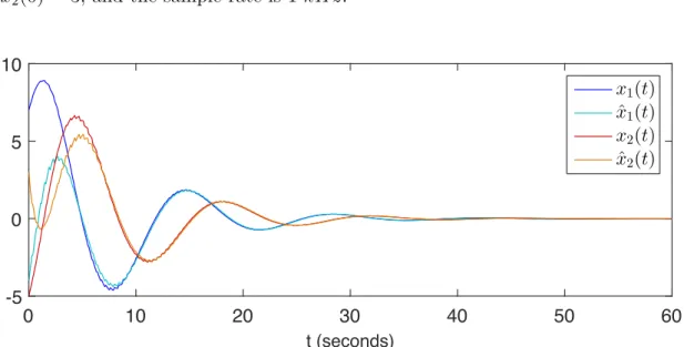
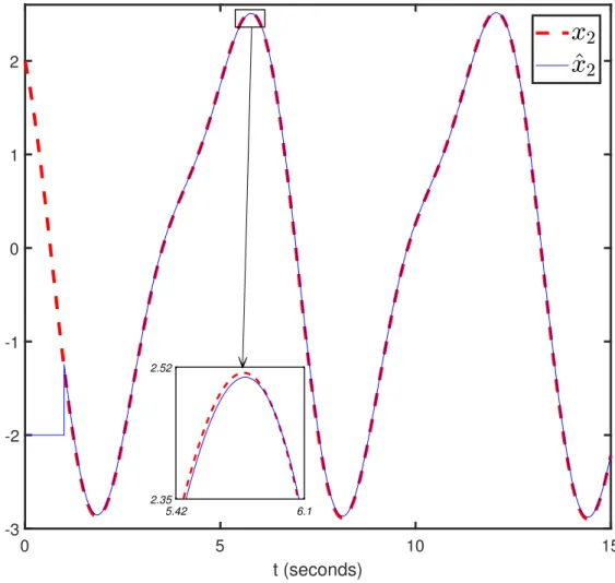
2.1 Simulation of the system (2.16): Component x and its estimate ˆx 33 3.1 Simulations of finite-time observer (3.18) for (3.71): Component
x2 and its estimate ˆx2 . . . 58
3.2 Simulation using controller (3.58) and continuous-discrete observer (3.57) for (3.75) . . . 59 4.1 Simulation of the closed loop time varying system (4.98) . . . 79 5.1 Simulations of continuous-discrete observer (5.27) for (5.41):
Chapter 1
Introduction
The problem of estimating the value of solutions of a system when some vari-ables cannot be measured is of great relevance, both from a theoretical and an applied point of view. Moreover, when the state of the system is not available for measurement, one aims to design output feedback controls that are computed from output observations. This motivates the problem of designing observers and stabilizing dynamic output feedbacks for switched and nonlinear systems because these systems are ubiquitous in communication networks and congestion control, automotive control, power converters, aircraft and air traffic control, process con-trol, mechanical systems, and many other engineering domains; see, e.g., [1], [2], [3], [4], [5], and [6] for the applications of switched systems, and see [7], [8], [9], [10], [11], and [12] for the applications of nonlinear systems.
We present four new observer designs in this thesis. First, we propose an observer for switched systems with delay in the output. Second, motivated by the fact that finite time convergence of estimation error is often desirable in applications like fault detection and feedback control, we design a finite time converging observer for a class of nonlinear time varying systems. Moreover, since the measured components of the state do not need to be estimated, we will also focus on reduced order finite time observer design for a family of nonlinear time varying systems. Finally, we will present a finite-time converging observer
design for linear time varying systems where the measurements are only available at discrete instants.
The stabilization problems we study in this thesis are motivated by the fact that the state of the system is not available for measurement in many engineering applications. Instead, one aims to design output feedback controls that are com-puted from output observations. We provide solutions to three dynamic output feedback stabilization problems for time varying systems in this thesis. To the best of our knowledge, the stabilization problems that we study in this work have remained unsolved. First, we study output feedback stabilization of switched systems with a delay in the output via an observer. Second, motivated by the fact that the observer values may also be intermittent, meaning there may be intervals during which there are no output measurements, we study the problem of stabilization for a broad class of nonlinear time varying systems with intermit-tent output measurements via finite time observer, which can be difficult when the dropout periods (when there are no output observations) are long. Finally, we provide a solution for an output feedback stabilization problem for a family of MIMO nonlinear time varying systems using reduced order finite time observer.
1.1
Classical Results on Switched Systems
A switched system is a class of hybrid dynamical system consisting of a family of continuous-time subsystems (also called modes) and a rule that governs switching between them [13]. Mathematically, a switched system can be written as
˙x = fσ(x) (1.1)
where {fσ : σ ∈ Ξ} is a family of sufficiently regular (at least locally Lipschitz)
functions from Rn to Rn that is parametrized on some index set Ξ. Typically, Ξ
is a compact (often finite) subset of a finite-dimensional linear vector space. In the particular case, when all the individual subsystems are linear i.e.,
and the index set Ξ is finite i.e., Ξ = {1, . . . , n}, we obtain a switched linear system.
To define a switched system generated by the above family, we need the notion of a switching signal. Given an initial time t0, an initial state x(t0) = x0 ∈ Rn,
and a switching sequence π = {(i0, t0), . . . , (ik, tk), . . . ,|ik ∈ Ξ, k ∈ Z≥0}, the
function σ : [0,∞) → Ξ = {1, ..., n} such that σ(t) = ik when t ∈ [tk, tk+1) is
called a switching signal. The function σ is a piecewise constant function and it has a finite number of discontinuities (switching instants) on every bounded interval of time and it takes a constant value on every interval between two consecutive switching instants. The role of σ is to specify the index σ(t) ∈ Ξ of the active subsystem at each instant of time t. We assume that σ is continuous from the right everywhere i.e. σ(t) = limθ→t+σ(θ) for each θ > 0. We also assume
that the state of 1.1 does not jump at the switching instants i.e., the solution x(·) is everywhere continuous. Thus a switched linear system can be described by
˙x(t) = Aσ(t)(x(t)) . (1.2)
1.1.1
Notions of Stability
Stability of switched systems is a significant and challenging problem because switched systems may manifest a complicated dynamical behavior due to their hybrid nature which is highlighted by the following fact.
Fact 1.1 ([13], [14]). Even if all of the subsystems of the switched system are stable, an unconstrained switching may destabilize it. Conversely, it may be pos-sible to stabilize a switched system through a suitable constrained switching even if all of its subsystems are unstable.
1.1.1.1 Stability for Arbitrary Switching
If all of the subsystems of a switched system are asymptotically stable, then the existence of a common Lyapunov function implies asymptotically stability of the switched system, uniform over the set of all switching signals. The existence of a common Lyapunov function is a necessary and sufficient condition for the switched system to be asymptotically stable under any arbitrary switching signal. This notion of stability is of great relevance for the case when a system is being controlled by means of switching among a set of stabilizing controllers; see [15] for more discussion on this topic.
1.1.1.2 Stability for Slow Switching
By restricting the class of admissible switching signals, asymptotic stability of the switched system can be achieved provided that all of its subsystems are asymp-totically stable. One way to restrict the class of switching signals is to make sure that the intervals between consecutive switching times are large enough. Such slow switching assumption is called dwell time approach and it greatly simplifies stability analysis. It is a well known fact that when all of the subsystems of the switched linear system are asymptotically stable, then it is globally asymptoti-cally stable (GAS) if the dwell time is large enough. The required lower bound on dwell time can be obtained from the parameters of individual subsystems; see [16, Lemma 2] for details. Multiple Lyapunov function tools play a vital role in stability analysis of slowly switched systems. The dwell time approach is ubiqui-tous in switching control literature; see for instance [17], [18], and the references therein.
1.1.1.3 Stabilizing Switching Signals
It is possible to find a switching signal that renders the switched system asymp-totically stable. Such a signal may even exist in extreme situations when all the
individual subsystems are unstable. For instance, assume that the system (1.2) has two modes. If the matrix pencil of the these modes contains a stable matrix then there exists a piecewise constant switching signal which makes the switched system quadratically stable, see [15, Theorem 11], [19], and [20] for more insight on this notion of stability.
1.1.2
Controllability, Reachability and Observability
Consider a switched linear system described by !
˙x(t) = Aσ(t)x(t) + Bσ(t)u(t)
y(t) = Cσ(t)x(t)
(1.3) with the state x valued in Rdx, the control input u valued in Rdu, the output y
valued in Rdy, and piecewise switching signal σ taking value from the finite index
set Ξ = {1, ..., n}. Let φ(t; t0, x0, u, σ) denote the state trajectory at time t of
switched system (1.3) starting from x(t0) = x0 with input u and switching signal
σ.
1.1.2.1 Controllability and Reachability
The controllability of switched linear systems is defined as Definition 1.1 ([21]). State x ∈ Rdx is controllable at time t
0, if there exist a
time instant tf > t0, a switching signal σ : [t0, tf) → Ξ, and input u : [t0, tf) →
Rdu, such that φ(t
f; t0, x, u, σ) = 0. The controllable set of system (1.3) at t0 is
the set of states which are controllable at t0. The system is said to be (completely)
controllable at time t0, if its controllable set at t0 is Rdx.
Let V (Ai, Bi)Ξ denotes the minimum subspace of Rdx, which is invariant under
all Ai, i∈ Ξ and which contains all image spaces of Bi, i∈ Ξ and let"(Ai, Bi)Ξ
Theorem 1.1 ([21]). For switched linear system "(Ai, Bi)Ξ, the controllable
set and reachable set are always identical, and they are precisely the subspace V(Ai, Bi)Ξ.
Corollary 1.1.1 ([21]). For switched linear system "(Ai, Bi)Ξ, the following
statements are equivalent:
(i) the system is completely controllable; (ii) the system is completely reachable; and (iii) V (Ai, Bi)Ξ = Rdx.
1.1.2.2 Observability
The observability of switched linear systems is defined as
Definition 1.2 ([22]). State x is said to be unobservable at t0, if for any
switch-ing signal σ, there is an input u, such that Cσφ(t; t0, x, u, σ) = Cσφ(t; t0, 0, u, σ)
for all t≥ t0. The unobservable set of system (1.3) at t0 is the set of states which
are unobservable. The system is said to be (completely) observable at t0, if its
unobservable set at t0 is null.
Let "(Ci, Ai)Ξ denotes the switched linear system (1.3) without input, and let
O(Ci, Ai)Ξ be the minimal subspace which is invariant under AiT, i∈ Ξ and which contains image spaces of CiT, i∈ Ξ. Let
U(Ci, Ai)Ξ = (O(Ci, Ai)Ξ)⊥
= {y ∈ Rdx :⟨x, y⟩ = 0, ∀x ∈ O(C
i, Ai)Ξ} .
where ⟨·, ·⟩ denotes the standard inner product in Rn.
Theorem 1.2 ([21]). For switched linear system (1.3), the unobservable set is subspace U (Ci, Ai)Ξ.
Corollary 1.2.1 ([22]). For switched linear system (1.3), the following state-ments are equivalent:
(i) the system is completely observable;
(ii) the system "(AiT, CiT)Ξ is completely controllable and/or reachable; and
(iii) O(Ci, Ai)Ξ = Rdx.
1.1.3
Feedback Stabilization
It is a well known fact that complete controllability implies state feedback sta-bilizabilty for a linear time invariant system. This problem has not been fully resolved in literature for general switched systems but some results have been achieved for a special class of switched systems as stated below:
Theorem 1.3 ([23]). If the summation of the controllable set of all the individual subsystems is the total state space, then the switched system is linear state feedback stabilizable.
Similarly, an interesting result is provided in ([24]) for the dynamic output feed-back stabilization of a class of switched linear systems for the case where all of the subsystems are controllable and observable. This result is stated below: Theorem 1.4 ([24]) For continuous-time switched linear system (1.3), suppose that each subsystem is controllable and observable. then, for any given scalar τ > 0, there is a dynamic output feedback law such that the closed-loop system is stable under every switching signal with dwell time τ .
In contrast to [24], the dynamic feedback stabilization methodology we state and prove in this dissertation does not require all of the modes of the switched linear system to be stabilizable and detectable. Therefore, our results can be applied
to a broad class of switched linear systems wider than those invoked in [24] and this is one of our significant contributions.
1.2
Classical Results on Nonlinear Systems
The basic families of nonlinear systems are nonautonomous systems, autonomous systems, and systems with inputs. An nth order nonautonomous nonlinear sys-tem can be described by n first-order one-dimensional differential equations as
⎧ ⎪ ⎪ ⎪ ⎪ ⎪ ⎨ ⎪ ⎪ ⎪ ⎪ ⎪ ⎩ ˙x1 = f1(t, x1, x2, . . . , xn) ˙x2 = f2(t, x1, x2, . . . , xn) .. . ˙xn = fn(t, x1, x2, . . . , xn) (1.4)
where x1, x2, . . . , xn are the state variables, t is the time, and all functions
f1, f2, . . . , fn are nonlinear in all of their arguments. More compactly, the system
(1.11) can be written as
˙x = f (t, x) (1.5) where the state vector x = (x1, x2, . . . , xn) is valued in a given open set X ⊆ Rn.
Given a constant t0 ≥ 0, x0 ∈ X , if x(t, t0, x0) can be uniquely defined for all
t ≥ t0 for all initial conditions x(t0, t0, x0) = x0, then the system (1.11) is called
forward complete. An equilibrium point x∗ = (x1∗, x2∗, . . . , xn∗) of (1.5) is defined
to be a vector in Rn for which f (t, x∗) = 0 for all t ≥ 0. Since f depends on
time, the systems defined by (1.5) are also called time-varying systems. If there is a constant T > 0 such that f satisfies f (t + T, x) = f (t, x) for all (t, x) in its domain, then the time-varing system (1.5) is called periodic with a period T .
If the right hand side of (1.11) or (1.5) is independent of time variable t, the the systems are called autonomous or time-invariant systems. Compactly, the autonomous systems can be written as
The general nonlinear time-varying systems with inputs can be described as ⎧ ⎪ ⎪ ⎪ ⎪ ⎪ ⎨ ⎪ ⎪ ⎪ ⎪ ⎪ ⎩ ˙x1 = f1(t, x1, x2, . . . , xn, u1, u2, . . . , up) ˙x2 = f2(t, x1, x2, . . . , xn, u1, u2, . . . , up) ... ˙xn = fn(t, x1, x2, . . . , xn, u1, u2, . . . , up) (1.7)
or, more compactly as
˙x = f (t, x, u) (1.8) where the variables u1, u2, . . . , up are inputs and the input vector u =
(u1, u2, . . . , up) is valued in a given set U ∈ Rp. The input u may represent a
control or disturbance. If the system (1.7) can be written as
˙x(t) =F(t, x) + G(t, x)u (1.9) for some vector fields F and G, then the system (1.7) is called affine in control or control affine.
1.2.1
Notions of Stability
Before describing various stability notions for nonlinear systems, we first recall the following classes of comparison functions. We say that a continuous function γ : [0,∞) → [0, ∞) belongs to class K and write γ ∈ K provided it is increasing and γ(0) = 0. We say that it belongs to class K∞ if, in addition, γ(r) → ∞ as
r → ∞. We say that a continuous function β : [0, ∞) × [0, ∞) → [0, ∞) is of class KL provided for each fixed s ≥ 0, the function β(·, s) belongs to class K, and for each fixed r ≥ 0, the function β(r, ·) is non-increasing and β(r, s) → 0 as s → ∞. For any constants p > 0, r ∈ N, and q ∈ Rr, we use the notation
ρBr(q) ={x ∈ Rr :|x − q| ≤ ρ}, which is denoted by ρBr when q = 0. Let M(U)
denote the set of all measurable essentially bounded functions u : [0.∞) → U; i.e. inputs that are bounded in | · |∞ where | · |∞ denote the sup norm of any matrix
valued function over its entire domain.
Definition 1.3 ([25]). Assume that the system (1.5) admits the origin 0 as an equilibrium point. The equilibrium 0 is stable provided for each constant ϵ > 0, there exists a constant δ(ϵ) > 0 such that for each initial state x0 ∈ X ∩δ(ϵ)Bn and
each initial time t0 ≥ 0, the unique solution x(t, t0, x0) satisfies |x(t, t0, x0)| ≤ ϵ
for all t≥ t0. Otherwise we call the equilibrium unstable.
Definition 1.4 ([25]). Assume that the system (1.5) admits the origin 0 as an equilibrium point. The equilibrium 0 is globally uniformly asymptotic sta-ble (GUAS) if there exists a function β ∈ KL such that for each initial state x0 ∈ X and each initial time t0 ≥ 0, the solution x(t, t0, x0) for (1.5) satisfies
|x(t, t0, x0)| ≤ β (|x0|, t − t0)) for all t≥ t0 ≥ 0. When the system is autonomous,
this property is called global asymptotic stability (GAS). The equilibrium 0 is uniformly asymptotically stable if there exists a function β ∈ KL and a constant ¯
c > 0 independent of t0 such that |x(t, t0, x0)| ≤ β (|x0|, t − t0)) for all t ≥ t0 ≥ 0
holds for all initial conditions x0 ∈ ¯cBn∩ X . When the system is time-invariant,
the preceding property is called (local) asymptotic stability (LAS).
Definition 1.5 ([25]). The basin of attraction of a LAS equilibrium point of a system is the set of all initial states that generate solutions of the system that converge to the equilibrium point.
Definition 1.6 ([25]). Assume that the system (1.5) admits the origin 0 as an equilibrium point. The equilibrium 0 is uniformly exponentially stable if there exist positive constants K1, K2, and r such that for each initial state x0 ∈ X ∩rBn
and each t0 ≥ 0, the corresponding solution x(t, t0, x0) satisfies |x(t, t0, x0)| ≤
K1e−K2(t−t0) for all t≥ t0. When the system is autonomous, this property is called
local exponential stability (LES) or, it is called global exponential stability (GES) if r can be taken to be +∞. The special case of uniform exponential stability where we can take r = +∞ is called global uniform exponential stability (GUES). Definition 1.7 ([25]). If there exist functions β ∈ KL and γ ∈ K such that for each u ∈ M(U) and each initial condition x(t0) = x0 ∈ X , the solution
x(t, t0, x0, u) of the system (1.8) with input vector u satisfies |x(t, t0, x0, u)| ≤
β (|x0|, t − t0) + γ(|u|[t0,t]) for all t ≥ t0 then the system (1.8) is input-to-state
(ISS) stable.
1.2.2
Stabilization
Stabilization is the problem of constructing a control law us(t, x) such that the
origin of (1.8) is asymptotically stable. If local stabilization is required then techniques based on linear approximation of (1.8) can be used. However, if GUAS is required then nonlinear design techniques like backstepping and forwarding can be applied. These techniques apply to nonlinear systems with special structure. Backstepping applies to lower triangular systems (feedback systems) of the form
⎧ ⎪ ⎪ ⎪ ⎪ ⎪ ⎨ ⎪ ⎪ ⎪ ⎪ ⎪ ⎩ ˙x1 = f1(t, x1, x2) ˙x2 = f2(t, x1, x2, x3) ... ˙xn = fn(t, x1, x2, . . . , xn, u) . (1.10)
Forwarding applies to upper triangular systems (feedforward systems) of the form ⎧ ⎪ ⎪ ⎪ ⎪ ⎪ ⎨ ⎪ ⎪ ⎪ ⎪ ⎪ ⎩ ˙x1 = f1(t, x1, . . . , xn, u) ˙x2 = f2(t, x2, . . . , xn, u) ... ˙xn = fn(t, xn, u) . (1.11)
Recently, it has been shown that Lyapunov based techniques can be used to handle stabilization problem for nonlinear systems; see [25] for details.
1.3
Classical Results on Time Delay Systems
Let Cin = C([−τ, 0], Rn) be the set of continuous functions mapping [−τ, 0] to
can be described by the retarded functional differential equation (RFDF) of the form
˙x(t) = f (t, xt) (1.12)
where x(t) ∈ Rn and f : R× C
in → Rn. The equation (1.12) specifies that the
derivative of state variable x at time t depends on t and x(ξ) for t− τ ≤ ξ ≤ t. For future evolution of state, the initial state variable in a time interval of length τ , say, from t0− τ to t0 is specified as xt0 = φ or x(t0+ θ) = φ(θ),−τ ≤ θ ≤ 0
where φ∈ Cin is given.
1.3.1
Notions of Stability
In this section, we introduce various notions of stability for time delay systems. Let the usual Euclidean norm of vectors, and the induced norm of matrices are denoted by| · |. For a function φ ∈ C([a, b], Rn), define the continuous norm | · |
c
by |φ|c = max
a≤θ≤b|φ(θ)|.
Definition 1.8 [26]. For the system described by (1.12), the trivial solution x(t) = 0 is said to be stable if for any t0 ∈ R and any ϵ > 0, there exists a
δ = δ(t0, ϵ) > 0 such that |xt0|c < δ implies |x(t)| < ϵ for t ≥ t0. It is said to be
asymptotically stable if it is stable, and for any t0 ∈ R and any ϵ > 0, there exists
a δa = δa(t0, ϵ) > 0 such that |xt0|c < δa implies lim
t→∞x(t) = 0. It is said to be
uniformly stable if it is stable and δ(t0, ϵ) can be chosen independently of t0. It is
uniformly asymptotically stable if it is uniformly stable and there exists a δa> 0
such that for any η > 0, there exists a T = T (δa, η), such that |xt0|c < δ implies
|x(t)| < η for t ≥ t0 + T and t0 ∈ R. It is globally (uniformly) asymptotically
stable if it is (uniformly) asymptotically stable and δa can be an arbitrarily large,
1.3.2
Classical Stability Theorems
In this section, we introduce some classical stability theorems for time delay systems.
Theorem 1.5 ([26]) (Lyapunov-Krasovskii Stability Theorem). Suppose f : R× Cin → Rn in (1.12) maps R×(bounded sets in Cin) into bounded sets of Rn,
and that u, v, w : R+ → R+ are continuous nondecreasing functions, where
additionally u(s) and v(s) are positive for s > 0, and u(0) = v(0) = 0. If there exists a continuous differentiable functional V : R× Cin → R such that
u(|φ(0)|) ≤ V (t, φ) ≤ v(|φ|c) (1.13)
and
˙
V (t, φ)≤ −w(|φ(0)|), (1.14) then the trivial solution of (1.12) is uniformly stable. If w(s) > 0 for s > 0 then it is uniformly asymptotically stable. If, in addition, lims→∞u(s) =∞, then it is
globally uniformly asymptotically stable.
Theorem 1.6 ([26]) (Lyapunov-Razumikhin Stability Theorem). Suppose f : R× Cin → Rn takes R×(bounded sets of Cin) into bounded sets of Rn, and that u, v, w : R+ → R+ are continuous nondecreasing functions, u(s) and v(s) are
positive for s > 0, and u(0) = v(0) = 0, v is strictly increasing. If there exists a continuously differentiable functtion V : R× Rn→ R such that
u(|x|) ≤ V (t, x) ≤ v(|x|), for t ∈ R and x ∈ Rn (1.15) and the derivative of V along the solution x(t) of (1.12) satisfies
˙
V (t, x(t))≤ −w(|x(t)|) if V (t + θ, x(t + θ)) ≤ V (t, x(t)) (1.16) for θ ∈ [−τ, 0], then the system (1.12) is uniformly stable.
If, in addition, w(s) > 0 for s > 0, and there exists a continuous nondecreasing function p(s) > s for s > 0 such that the condition (1.16) is strengthened to
˙
for θ ∈ [−τ, 0], then the system (1.12) is uniformly asymptotically stable.
If in addition lims→∞u(s) = ∞, then the system (1.12) is globally uniformly
asymptotically stable.
Lemma 1.1 ([27]) (Halanay’s inequality). If there exists a nonnegative contin-uous function f (t) on [t0 − τ, t0] such that
˙
f (t)≤ −αf(t) + β sup
s∈[t−τ,t]
f (s) (1.18) for t≥ t0 and if α > β > 0, then there exists α > 0 and k > 0 such that
f (t)≤ ke−γ(t−t0) (1.19)
for t≥ t0.
1.4
Summary of Contributions
This section provides a cursory glance at the contributions and constitution of the entire dissertation.
Chapter 2
We propose a new technique to design observers and stabilizing dynamic output feedbacks for switched linear systems with a time-varying pointwise delay in the output. First, we develop an extension of the trajectory based stability result recently proposed in [28] to establish the stability of the closed-loop switched system. We wish to emphasize that the new extension of the trajectory based approach we state and prove in this chapter is of interest by itself: it can be applied to a wide range of systems, notably to families of systems with time-varying delays wider than those invoked in [28] and [29], and therefore it is one of the important contributions of this chapter. In its simplest version, this new technique entails to verifying that there exist constants ϵ∈ (0, 1) and T > 0 such that each trajectory x of a system satisfies an inequality of the form |x(t)| ≤
ϵ supℓ∈[t−T,t]|x(ℓ)| for all t ≥ T . Second, the stabilization result we develop in Chapter 2 is, to the best of our knowledge, new.
Chapter 3
We have two main objectives this chapter. Our first aim is to construct finite time smooth observers for nonlinear systems. To the best of our knowledge, very few works design finite time smooth observers for nonlinear systems; see, e.g., [30] for a finite time smooth observer for nonlinear systems. The preceding finite time observer design approach was carried out without considering disturbances in the measurements or dynamics. Such disturbances are usually present in prac-tical applications and they affect measurements, and can be state dependent. Motivated by this fact, we provide a finite time state estimation algorithm for nonlinear systems with state dependent disturbances. Nonlinear systems with state dependent disturbances that we consider in this chapter arise in many en-gineering contexts, e.g., in the modeling of vibrations of elastic membranes; see [31]. Our observer design approach has two main advantages. First, our finite time observers are smooth and they have better robust performance as compared to nonsmooth observers. Second, the convergence time in our method is indepen-dent of the initial state and it can be rendered as small as desired by the selection of a parameter (called the artificial delay). Our second result is dynamic output feedback design for a class of nonlinear systems with temporary loss of output measurements. It is motivated by the fact that in many engineering applications, the state is not available for measurement, and the output measurements are only available intermittently, meaning there may be intervals during which there is no output measurement, e.g., due to communication failures in GPS-denied environments. Our strategy has the following steps. We combine our finite time observer design and classical results for switched systems to construct a dynamic output feedback using a continuous-discrete observer. To establish the stability of the closed-loop system, we use an extension of the trajectory based approach proposed in [28]. To the best of our knowledge, the stabilization problem we describe with temporary loss of output measurements has remained unsolved in the literature, even in the case of linear systems, so our proposed tools are of considerable independent interest.
Chapter 4
Since systems are frequently time-varying and tracking problems can be recasted into stabilization problems of equilibria of time-varying systems, and since the measured components of the state do not need to be estimated, this chapter is devoted to the construction of finite-time reduced order observers for a family of nonlinear time-varying systems. The observer we will build gives estimates only of the unmeasured variables, as does the asymptotic observer proposed for instance in [32, Chapt. 4, Sec. 4.4.3]. This feature presents the following technical advantages. The design is simpler and in some cases, due to the need to determine fundamental solutions of time-varying systems, considering systems with a smaller dimension than the studied one makes it possible to solve the problem, which would be impossible if we were attempting to construct a full-order observer, due to the difficulty of determining explicit formulas for fundamental solutions of systems of dimension larger than 1. In addition, the reduced order observer we propose yield better performances than full order observers, in some cases. To the best of our knowledge, finite-time reduced order observers are proposed for the first time in the present paper. Additionally, we give a second new result where we show how the finite-time observer we propose can be used to solve a dynamic output feedback stabilization problem for a MIMO nonlinear system. Chapter 5
This chapter has two goals. First, we construct a finite time observer for a linear continuous-time system with sampled output in the presence of a disturbance in the dynamics of the system. The observer is expressed in terms of the funda-mental solution of suitable time-varying system. Second, we obtain more explicit formulas for finite time observers that do not contain the fundamental matrix and therefore may be better suited to implementations where the fundamental matrix is not available in explicit closed form.
We summarize the value added by our paper and suggest future research direc-tions in this chapter.
1.5
Notation
Throughout the sequel, the notation will be simplified whenever no confusion can arise from the context.
• The dimensions of our Euclidean spaces are arbitrary unless otherwise noted.
• The usual Euclidean norm of vectors, and the induced norm of matrices, are denoted by | · |.
• I denotes the identity matrix of any dimension.
• xT or AT denotes the transpose of a vector x or a matrix A.
• For any constant τ > 0, any continuous function φ : [−τ, +∞) → Rn and
all t≥ 0, we define φt by φt(m) = φ(t + m) for all m ∈ [−τ, 0].
• We let Cindenote the set C([−τ, 0]) of all continuous functions φ : [−τ, 0] →
Rn.
• A vector or a matrix is nonnegative (resp. positive) if all of its entries are nonnegative (resp. positive).
• We write M ≻ 0 (resp. M ≼ 0) to indicate that M is a symmetric positive definite (resp. negative semi-definite) matrix.
• For two vectors V = (v1...vn)⊤ and U = (u1...un)⊤, we write V ≤ U to
indicate that for all i∈ {1, ..., n}, vi ≤ ui.
• A matrix is called Schur stable provided its spectral radius σ satisfies σ < 1. • Let | · |∞ denote the sup norm of any matrix valued function over its entire
• Let exp(f) denotes the real valued function ef for any real valued function
f .
• For any continuous function Ω : [−τ, +∞) → Rn×n, we let Φ
Ω denote the
function such that
∂ΦΩ
∂t (t, t0) =−ΦΩ(t, t0)Ω(t)
and ΦΩ(t0, t0) = I for all t ∈ R and t0 ∈ R. Then M(t, s) = Φ−1Ω (t, s) is
the fundamental solution associated to Ω for the system ˙x = Ω(t)x; see [33, Lemma C.4.1].
Chapter 2
Observer based Stabilization of
Switched Systems with Delay
The content of this chapter is based on the publications [34] and [35] which were published by the author and his advisors while the study of this dissertation was in progress. Many questions related to switched systems such as stability ([36]; [13]; [15]; [37]), controllability ([38]; [21]), observability and reachability ([21]; [39]; [40]; [41]), and synthesis ([42]; [22]) have been extensively studied in various contributions. Stability and stabilization are amongst the most challenging prob-lems pertaining to switched systems due to their hybrid nature [43], and they are the main topic of the present chapter.
Before describing the results we will propose, let us review two basic approaches classically utilized in the literature for establishing the stability of switched sys-tems and some issues related to these techniques:
(i) It is shown in [15] that existence of a common strict Lyapunov function (a Lyapunov function whose derivative along the trajectory of all of the subsys-tems of the switched system is definite negative) is a necessary and sufficient condition for the switched system to be stable under arbitrary switching. On the other hand, when such a Lyapunov function exists, finding it may
be a difficult task because it is an NP-hard problem; see [44].
(ii) It is also shown in [15] that even if a switched system does not possess a common strict Lyapunov function, it may be stable, under requirements such as for instance a condition on the size of the difference between two consecutive switching instants. This fundamental result is termed as dwell-time approach in the literature. When this size is sufficiently large, then a so-called dwell-time result can be established. Typically, the proof uses multiple strict Lyapunov functions. It is worth mentioning that multiple Lyapunov functions may lead to an undesirable attenuation property which can only be mitigated by imposing some strong assumptions; see [45]. Both of the above mentioned approaches are mainly developed for non-delayed systems. But measurement delays are present in many practical applications, such as chemical processes, aerodynamics and communication networks, and they are time-varying (see for instance [46] and [47]). Therefore, the problem of stabilizing switched systems when a time-varying delay is present in the output is strongly motivated. On the other hand, it is a difficult problem because it does not seem possible to directly extend the classical Lyapunov function based approaches mentioned above to the output feedback case considered in this chapter. This comment is not in contradiction with the fact that some control problems for switched systems with delay in the input have been solved. Let us recall some of them, which complement our contribution.
2.1
Literature Review
Feedback stabilization of delayed switched linear systems is proposed in [48] us-ing a combination of the multiple Lyapunov functions approach and the mergus-ing switching signal technique. An online and offline feedback controller design for de-layed switched linear systems in the detection of the switching signal are discussed in [49]. Moreover, [50] and [51] present feedback controller designs for delayed switched systems using a dwell-time based stability analysis approach. Note that
[48], [49], [50], and [51] assume that all of the subsystems of the switched system are controllable. A stabilization problem for a class of delayed switched systems is studied in [52] and [53] under the assumption that the subsystems satisfy a certain Hurwitz convex combination condition. A common Lyapunov function approach is used in [52] and [53] to carry out stability analysis. It is assumed in [52] that the delay is constant and [53] requires the derivative of the delay to be bounded. Also note that [48], [49], [50], [51], [52], and [53] present state feedback designs only and it seems to us that there is no direct way to extend them to the output feedback case considered in this chapter. Moreover, most of these contributions use classical Lyapunov function based approaches to establish sta-bility of the closed-loop switched systems. However, it becomes difficult to search appropriate Lyapunov functions for the case when there is a time varying delay in the output of the switched systems.
2.2
Contributions of this chapter
We think that our main result can be regarded as an extension of [48], [49], [50], [51], [52], [53], and [54], offering new advantages that are listed below:
(i) Our main result does not require all of the subsystems to be stabilizable and detectable.
(ii) Our feedback stabilization approach does not assume that all the states are available for feedback.
(iii) We use a new extension of trajectory based approach for stability analysis which circumvents the serious obstacle presented by the search for appro-priate Lyapunov functions.
(iv) We allow the delay to be time-varying and piecewise continuous function of time, and we do not impose any constraint on the upper bound of the delay derivative.
(vi) The application of our results is not restricted to the class of delayed switched systems where all the convex combinations of the subsystems in the absence of control must be Hurwitz.
The rest of this chapter is organized as follows. An extension of the trajectory based approach is given in Section 2.3. Section 2.4 is devoted to the main result of the chapter. Section 2.5 discusses computational issues related to the delay bound. The results are illustrated by a numerical example in Section 2.6.
2.3
Trajectory based approach and its extension
For stabilization of time varying systems with time varying delays, Lyapunov-Krasovskii functionals or Razhumukin functions [55] are used in much of the lit-erature. However, finding strict Lyapunov functions can be difficult. Instead, it is easier to verify that there exist constants ϵ∈ (0, 1) and T > 0 such that each tra-jectory x of a system satisfies an inequality of the form|x(t)| ≤ ϵ supℓ∈[t−T,t]|x(ℓ)|
for all t ≥ T . This provides motivation for trajectory based approach proposed in [28]. It relies on ISS stability notion and it yields ISS stability with respect to uncertainty. The two main advantages of trajectory based approach are 1) it can be applied to a broad class of time varying systems with time varying delays and 2) it is easier to apply as compared to Lyapunov or small-gain methods. We now provide the following key lemma which forms the basis of trajectory based approach.
Lemma 2.1 [28] (Trajectory based approach). Let T∗ > 0 be a constant. Let a
piecewise continuous function w : [−T∗, +∞) → [0, +∞) admits a sequence of real
numbers vi and positive constants ¯va and ¯vb such that v0 = 0, vi+1− vi ∈ [¯va, ¯vb]
for all i≥ 0, w is continuous on each interval [vi, vi+1) for all i≥ 0, and w(vi−)
exists and is finite for each i ∈ N. Let d : [0, +∞) → [0, +∞) be any piecewise continuous function, and assume that there is a constant ρ∈ (0, 1) such that
holds for all t≥ 0. Then
w(t)≤ |w|[−T∗,0]e ln(ρ)
T ∗ + 1
(1− ρ)2|d|[0,t] (2.2)
holds for all t≥ 0.
We now provide with an extension of the trajectory based approach given in [28].
Lemma 2.2 Let us consider a constant T > 0 and l functions zg : [−T, +∞) →
[0, +∞), g = 1, ..., l. Let Z(t) = (z1(t) ... zl(t))⊤ and, for any θ ≥ 0 and t ≥ θ,
define Vθ(t) = ' sup s∈[t−θ,t] z1(s) ... sup s∈[t−θ,t] zl(s) (⊤ . Let Υ ∈ Rl×l be a nonnegative
Schur stable matrix. If for all t≥ 0, the inequalities Z(t) ≤ ΥVT(t)
are satisfied, then
lim
t→+∞zg(t) = 0
for all g = 1, . . . , l.
Proof. Since Υ is Schur stable, there is an integer q > 1 such that
|Υq|√l < 1 . (2.3)
From Lemma A.1 of the Appendix A, we deduce that Z(t)≤ ΥqV
qT(t) (2.4)
for all t≥ qT . Consequently,
|Z(t)| ≤ |Υq||V qT(t)|. Using |VqT(t)| = ) * * + l , i=1 sup s∈[t−qT,t] zi(s)2 ≤ √l sup s∈[t−qT,t]|Z(s)|, (2.5)
we obtain
|Z(t)| ≤ |Υq|√l sup
s∈[t−qT,t]|Z(s)|.
(2.6) This inequality, in combination with the inequality (2.3) and Lemma 2.1 allows us to conclude the result. !
2.4
Observer and control design
We introduce a range dwell-time condition, i.e. a sequence of real numbers tk
such that there are two positive constants δ and δ such that t0 = 0 and for all
k ∈ Z≥0,
tk+1− tk ∈ [δ, δ] . (2.7)
Definition 2.1 Let π ={(i0, t0), . . . , (ik, tk), . . . ,|ik ∈ Ξ, k ∈ Z≥0} be a
switch-ing sequence. The function σ : [0,∞) → Ξ = {1, ..., n} such that σ(t) = ik when
t∈ [tk, tk+1) is called an associated switching signal.
We consider the continuous-time switched linear system with output delay: !
˙x(t) = Aσ(t)x(t) + Bσ(t)u(t)
y(t) = Cσ(t)x(t− τ(t))
(2.8) with x ∈ Rdx, u ∈ Rdu, y ∈ Rdy, for all t ≥ 0, τ(t) ∈ [0, τ] with τ > 0 and an
initial condition in Cin. The delay τ (t) is supposed to be a piecewise continuous
function. For any i∈ Ξ, Ai, Bi, and Ci are real and constant matrices of
compat-ible dimensions and σ is a switching signal. We introduce an assumption which pertains to the stabilizability and the detectability of the system (2.8), but does not imply that all the pairs (Ai, Bi) are stabilizable and all the pairs (Ai, Ci) are
Assumption 2.1 There are matrices Ki and Li for all i ∈ Ξ and constants
T ≥ ¯τ, a ∈ [0, 1), b ≥ 0, c ∈ [0, 1) and d ≥ 0 such that the solutions of the system ˙α(t) = Mσ(t)α(t) + ζ(t) (2.9)
with Mi = Ai+ BiKi and ζ being a piecewise continuous function, satisfy
|α(t)| ≤ a|α(t − T )| + b sup
ℓ∈[t−T,t]|ζ(ℓ)|
(2.10) for all t≥ T . Similarly, the solutions of the system
˙
β(t) = Nσ(t)β(t) + η(t) (2.11)
with Ni = Ai + LiCi and η being a piecewise continuous function, satisfy the
following inequality for all t≥ T
|β(t)| ≤ c|β(t − T )| + d sup
ℓ∈[t−T,t]|η(ℓ)| .
(2.12)
Theorem 2.1 Let the system (2.8) satisfy Assumption 2.1 and, s1, s2 and s3 be
defined by s1 = sup i∈Ξ |Bi Ki| , s2 = sup i∈Ξ|Li Ci| , s3 = sup i∈Ξ|Mi| . (2.13) If τ (t) ≤ ¯τ < ¯τu (2.14)
for all t≥ 0, where
¯ τu =
(1− a)(1 − c) ds1s2((1− a) + bs3)
, (2.15) then the origin of the following feedback system is globally uniformly exponentially stable (GUES):
!
˙x(t) = Aσ(t)x(t) + Bσ(t)Kσ(t)x(t)ˆ
˙ˆx(t) = Aσ(t)x(t) + Bˆ σ(t)Kσ(t)x(t) + Lˆ σ(t)[Cσ(t)x(t)ˆ − y(t)] .
(2.16)
Proof. Let us introduce ˜x(t) = ˆx(t)− x(t). Then
As an immediate consequence, using the definitions of the matrices Mi and Ni,
we obtain !
˙x(t) = Mσ(t)x(t) + Bσ(t)Kσ(t)x(t)˜
˙˜x(t) = Nσ(t)x(t) + L˜ σ(t)Cσ(t)[x(t)− x(t − τ(t))] .
From Assumption 2.1 and the equality x(ℓ)− x(ℓ − τ(ℓ)) =-ℓ
ℓ−τ(ℓ)[Mσ(m)x(m) +
Bσ(m)Kσ(m)x(m)]dm, it follows that, for all t˜ ≥ T + ¯τ,
|x(t)| ≤ a|x(t − T )| + b sup ℓ∈[t−T,t]|Bσ(ℓ) Kσ(ℓ)x(ℓ)˜ | , (2.17) |˜x(t)| ≤ c|˜x(t − T )| + d sup ℓ∈[t−T,t] . . .Lσ(ℓ)Cσ(ℓ) ×-ℓ ℓ−τ(ℓ)[Mσ(m)x(m) + Bσ(m)Kσ(m)x(m)]dm˜ . . . . (2.18) Using the constants defined in (2.13), we deduce from (2.17) and (2.18) that (x(t), ˜x(t)) satisfies: |x(t)| ≤ a|x(t − T )| + bs1 sup ℓ∈[t−T −¯τ ,t]|˜x(ℓ)| , |˜x(t)| ≤ ds2s3τ¯ sup ℓ∈[t−T −¯τ ,t]|x(ℓ)| + (c + ds 1s2¯τ ) sup ℓ∈[t−T −¯τ ,t]|˜x(ℓ)| .
Lemma 2.2 ensures that the origin of (2.16) is GUES if /
a bs1
ds2s3τ ds¯ 1s2τ + c¯
0
is Schur stable, which is equivalent to
a+c+ds1s2τ¯ 2 + 1 2a+c+ds1s2τ¯ 2 32 − ac − ds1s2(a− bs3) ¯τ < 1 ,
from which we derive the simpler condition (2.14). !
2.5
Parameters of the delay bound
In this section, we illustrate a method to determine the constants a, b, c, and d appearing in Assumption 2.1.
Consider a continuous-time switched linear system
˙ξ(t) = Ωσ(t)ξ(t) + ϑ(t) , (2.19)
where ξ ∈ Rdξ, the switching signal σ is associated to a sequence t
k of the type
of those introduced in Section 2.4 and ϑ is a piecewise continuous function. Lemma 2.3 Let the system (2.19) be such that there are real numbers d1 > 0,
d2 > 0, µ ≥ 1, γ > 0 and symmetric positive definite matrices Ql, l ∈ Ξ, such
that the LMIs
d1I ≼ Qi ≼ d2I , (2.20)
Qi ≼ µQj , (2.21)
Ω⊤i Qi + QiΩi ≼ −γQi (2.22)
are satisfied for all i, j ∈ Ξ. Moreover, the constant µ△ = µe−γδ is such that
µ△ < 1 . (2.23) Then, along the trajectory of (2.19), the inequality
|ξ(t)| ≤4 d2 d1 µµρ△eγδ|ξ(t − T )| + 5 µ d2 γd1 T sup ℓ∈[t−T,t]|ϑ(ℓ)|
holds for all t≥ T where T > 0 and ρ is a positive integer depending on the choice of T such that for all t∈ [tk, tk+1), we have t− T ∈ [tk−ρ−1, tk−ρ). Moreover, we
have 1d2 d1µµ ρ △eγδ < 1 when ρ > ln(µ1∆) 6 ln7d1 d2µ 8 − γδ9.
Proof. Let us define Lyapunov functions:
Vi(ξ) = ξ⊤Qiξ, ∀i ∈ Ξ .
We deduce from (2.22) that when σ(t) = i, then the derivative of Vi along the
trajectories of (2.19) satisfies ˙
Vi(ξ(t)) ≤ −2γVi(ξ(t)) + 2ξ(t)⊤Qiϑ(t)
≤ −γVi(ξ(t)) + γ1ϑ(t)⊤Qiϑ(t)
where the last inequality is deduced from the Young’s inequality. Now, let us integrate (2.24) between two instants s and t, t ≥ s, belonging to the same sampling interval where σ(t) = l. Then
eγtV l(ξ(t)) ≤ eγsVl(ξ(s)) + 1γ : t s eγmϑ(m)⊤Qlϑ(m)dm. It follows that Vl(ξ(t)) ≤ eγ(s−t)Vl(ξ(s)) + 1γ : t s eγm−γtϑ(m)⊤Qlϑ(m)dm ≤ eγ(s−t)V l(ξ(s)) + dγ2 : t s eγm−γt|ϑ(m)|2dm , (2.25)
where the last inequality is a consequence of (2.20). Now, let us consider T > 0, t ≥ T such that t ∈ [tk, tk+1) for some k ∈ Z≥0 and let ρ ∈ N be such that
t− T ∈ [tk−ρ−1, tk−ρ). From (2.25), we deduce that
Vσ(tk)(ξ(t)) ≤ e −γ(t−tk)V σ(tk)(ξ(tk)) + d2 γ : t tk eγm−γt|ϑ(m)|2dm ≤ µe−γ(t−tk)V σ(tk−1)(ξ(tk)) + d2 γ : t tk |ϑ(m)|2dm , (2.26)
where the last inequality is a consequence of (2.21). For similar reasons, Vσ(tk−1)(ξ(tk)) ≤ µ△Vσ(tk−2)(ξ(tk−1)) d2 γ : tk tk−1 |ϑ(m)|2dm .. . Vσ(tk−ρ)(ξ(tk−ρ+1)) ≤ µ△Vσ(tk−ρ−1)(ξ(tk−ρ)) + d2 γ : tk−ρ+1 tk−ρ |ϑ(m)|2dm (2.27) and Vσ(tk−ρ−1)(ξ(tk−ρ)) ≤ e γ(t−T −tk−ρ)V σ(tk−ρ−1)(ξ(t− T )) +d2 γ : tk−ρ t−T |ϑ(m)| 2dm . (2.28)
We deduce from (2.27) that Vσ(tk−1)(ξ(tk)) ≤ µ ρ △Vσ(tk−ρ−1)(ξ(tk−ρ)) + d2 γ : tk tk−ρ |ϑ(m)|2dm. (2.29)
Combining (2.26), (2.28) and (2.29), we obtain Vσ(tk)(ξ(t)) ≤ µe−γ(t−t k) ! µρ△Vσ(tk−ρ−1)(ξ(tk−ρ)) + d2 γ : tk tk−ρ |ϑ(m)|2dm ; +d2 γ : t tk |ϑ(m)|2dm ≤ µe−γ(t−tk)µρ △eγ(t−T −tk−ρ)Vσ(tk−ρ−1)(ξ(t− T )) +µe−γ(t−tk)µρ △dγ2 : tk−ρ t−T |ϑ(m)| 2dm +µe−γ(t−tk) d2 γ : tk tk−ρ |ϑ(m)|2dm + d2 γ : t tk |ϑ(m)|2dm.
Then using the definition of range dwell-time condition from (2.7), we get Vσ(tk)(ξ(t))≤ µ µ ρ △eγδVσ(tk−ρ−1)(ξ(t− T )) + µ d2 γ : t t−T|ϑ(m)| 2dm .
From (2.20), we deduce that
d1|ξ(t)|2 ≤ µµρ△eγδd2|ξ(t − T )|2+ µdγ2
: t
t−T|ϑ(m)| 2dm.
Using the inequality √p1+ p2 ≤√p1+ √p2 for all p1 ≥ 0, p2 ≥ 0, we obtain
|ξ(t)| ≤ 4 d2 d1 µµρ△eγδ|ξ(t − T )| + 5 µ d2 γd1 T sup ℓ∈[t−T,t]|ϑ(ℓ)| .
Since (2.23) holds and T is arbitrarily large, one can choose T such that the corresponding ρ is so that 1d2
d1µµ
ρ
△eγδ < 1. This concludes the proof. !
Remark 2.1
1. Note that (2.23) holds if and only if δ > ln(µ)γ , which defines a minimum dwell-time condition.
2. Conditions of Lemma 2.3 are always satisfied when the matrices Ωi, ∀ i ∈ Ξ,
are Hurwitz; i.e., one can always find symmetric positive definite matrices Qi,
i∈ Ξ, and real numbers d1 > 0, d2 > 0, µ≥ 1, γ > 0 satisfying the LMIs (2.20),
(2.21), and (2.22). In the next section we illustrate an alternative approach for the case where some of Ωi’s are not Hurwitz.
2.6
Illustrative Example
Consider the continuous-time switched linear system (2.8) with x∈ R2, τ ∈ [0, τ),
σ(t) = ⎧ ⎨ ⎩ 1 if 4ℓκ≤ t < (4ℓ + 3)κ 2 if (4ℓ + 3)κ≤ t < 4(ℓ + 1)κ , (2.30) where κ > 0 is to be determined, ℓ = 0, 1, 2, . . ., and
A1 = / 0 −1/2 2/5 0 0 , B1 = / 0 0 0 0 0 , C1 = / 1 0 0 1 0 , A2 = / 0 −2/5 1/2 0 0 , B2 = / 1 0 0 1 0 , C2 = / 0 0 0 0 0 .
Let us observe that the subsystem (A1, B1, C1) is not stabilizable but it is
de-tectable whereas the subsystem (A2, B2, C2) is stabilizable but not detectable.
Moreover, in the absence of control, no convex combination of the A1 and A2 is
Hurwitz. Furthermore, the subsystems cannot be stabilized by a static output feedback u = Kiy. In this example, we have δ = κ and δ = 3κ and the switchings
are periodic with a period of 4κ. We will determine a set of parameters for the delay bound depending on κ.
2.6.1
Preliminary result
First, we provide a preliminary result which shows how Assumption 2.1 can be satisfied in this particular example where some of the subsystems of the switched systems are not stabilizable and not detectable.
Lemma 2.4 Consider the switched linear system
˙z(t) = Γσ(t)z(t) + ϱ(t) (2.31)
with σ defined by (2.30), and let Γ1 ∈ R2×2, Γ2 ∈ R2×2 and κ > 0 be such that
of the system (2.31) with ϱ = 0: ∂Φ⋆
∂t (t, s) = Γσ(t)Φ⋆(t, s) , Φ⋆(s, s) = I , for all t∈ R and s ∈ R. Then, for all s ≥ 0, t ≥ s
|Φ⋆(t, s)| ≤ p1e−p2(t−s) (2.32)
with p1 = e8κ max{|Γ1|,|Γ2|}cκe2dκ and p2 = dκ/4κ, where cκ > 1 and dκ > 0 are such
that for all m∈ N,
|Sκm| ≤ cκe−dκm . (2.33)
Moreover, for all T > 0,
|z(t)| ≤ p1e−p2T|z(t − T )| +
p1(1−e−p2T)
p2 sup
ℓ∈[t−T,t]|ϱ(ℓ)| . (2.34)
Proof. Let us introduce a sequence: gℓ = 4ℓκ. Then for all integer n > 0,
z(gℓ) = Sκnz(gℓ−n) . (2.35)
Thus
Φ⋆(gℓ, gℓ−n) = Sκn. (2.36)
Let t∈ R and s ∈ R be such that t > s ≥ t − 4κ. Then
|Φ⋆(t, s)| ≤ e4κ max{|Γ1|,|Γ2|} . (2.37)
Now, let t ∈ R and s ∈ R be such that t + 4κ > s. Then there is ℓ such that t∈ [gℓ, gℓ+1) and r∈ N, r > 0 such that s ∈ [gℓ−r−1, gℓ−r). Then
|Φ⋆(t, s)| ≤ e8κ max{|Γ1|,|Γ2|}|Φ⋆(gℓ, gℓ−r)| . (2.38)
It follows that
|Φ⋆(t, s)| ≤ e8κ max{|Γ1|,|Γ2|}|Sκr| .
Since Sκ is Schur stable, there are cκ > 1 and dκ > 0 such that for all m∈ N,
|Sm
κ | ≤ cκe−dκm. (2.39)
Thus
Now, notice that r≥ t−s
4κ − 2. Consequently,
|Φ⋆(t, s)| ≤ e8κ max{|Γ1|,|Γ2|}cκe2dκe−dκ
t−s
4κ . (2.41)
From (2.37) and (2.41), we deduce that for all t≥ s, |Φ⋆(t, s)| ≤ e8κ max{|Γ1|,|Γ2|}cκe2dκe−dκ
t−s
4κ . (2.42)
This allows us to conclude that (2.32) is satisfied.
Now, by integrating (2.31), we obtain that for all t ≥ T , |z(t)| = .. .Φ⋆(t, t− T )z(t − T ) + -t t−T Φ⋆(t, ℓ)ϱ(ℓ)dℓ . . . ≤ p1e−p2T|z(t − T )| + -t t−T p1e−p2(t−ℓ)dℓ sup ℓ∈[t−T,t]|ϱ(ℓ)|
where the last inequality is a consequence of (2.32). ! Remark 2.2 Since p2 > 0, then p1e−p2T < 1 when T > ln(pp21), which determines
a lower bound for T .
2.6.2
Output feedback stabilization
Let us choose the gain matrices as K2 = / −1/2 0 0 −4/7 0 , L1 = / −3/5 0 0 −4/5 0 .
Setting Γ1 = M1 = A1 and Γ2 = M2 = A2 + B2K2, one can easily corroborate
that (2.33) is satisfied with the choice of κ = 0.1, ck = 1.01, and dk = 0.001 for
all m∈ N. Setting z = α, Ωi = Γi = Mi for i∈ {1, 2}, and ϱ = ζ, it can be easily
verified that (2.32) is satisfied by (2.9) with p1 = e8κ max{|Γ1|,|Γ2|}cκe2dκ = 1.7142
and p2 = dκ/4κ = 1.0025. Using Lemma 2.4 with T = 6, one can observe
that the solutions of system (2.9) satisfy (2.10) with a = p1e−p2T = 0.0042,
b = (p1/p2)21 − e−p2T3 = 1.7057. A similar analysis shows that the solutions of
we conclude that the switched delay system satisfies Assumption 2.1. Finally, application of Theorem 2.1 with s1 = 0.5714, s2 = 0.8, s3 = 0.7611, and with
the preceding choices of the parameters yields ¯τu = 0.4465. Fig. 2.1 shows the
simulation of system (2.16) for this particular example for a piecewise continuous sawtooth function τ (t) of a fundamental frequency of 1 Hz described by τ (t) = 0.2(t− ⌊t⌋) where the switching signal σ(t) is given by (2.30) with κ = 0.1. The initial conditions are chosen to be x1(0) = 7, x2(0) = −5, ˆx1(0) = −4, and
ˆ
x2(0) = 3, and the sample rate is 1 kHz.
t (seconds) 0 10 20 30 40 50 60 -5 0 5 10 x1(t) ˆ x1(t) x2(t) ˆ x2(t)
Chapter 3
Finite Time Observer Design and
Stabilization of Nonlinear
Systems with Intermittent
Output Measurements
The content of this chapter is based on the publication of the author [56]. State estimation of nonlinear systems from output measurements is a basic concern in robotics [57], chemical and biochemical processes [58], biomedical systems [59], communication systems [60], automotive systems [61], networked control systems [62], and many other fields. Due to this strong motivation, various techniques to achieve state observation of nonlinear systems have been discussed in the liter-ature. These techniques have included canonical form observers [63], high-gain observers (as in [64], [65], and [66]), Lyapunov based observers (as in [67] and [68]), and extended Kalman and Luenberger observers (as in [69] and [70]).
The above mentioned observer design techniques have the common disadvan-tage that they only ensure asymptotic convergence of the estimation error to zero, whereas finite time convergence of estimation errors to zero is often desirable for
control and supervision purposes; see [71], [72] and [73], and see [74] for more mo-tivation for finite time control. One can distinguish between two broad families of finite time converging observers, namely, the families composed of nonsmooth observers without delay and the family of the smooth observers with delays. Non-smooth finite time converging observers have been proposed for instance in [60], [71], [75], [76], and [77]. The main drawback of nonsmooth finite time observers is that their lack of smoothness may generate poor robustness performance, but they have no delay, which is an advantage because the presence of a delay may complicate the implementation of an observer. Another possible drawback is due to the fact that the time of convergence of each trajectory depends on its initial condition. This is not the case for the observers that use artificial delays, for which their instant of convergence of the solutions is independent of the initial conditions and can be rendered as small as desired by the selection of a parameter (called the artificial delay).
3.1
Literature Review
Finite time smooth observer designs have been introduced more recently. They were first presented in [78], which was only applicable to linear time invariant (LTI) systems; see also [79] for finite time observers for LTI systems. An extension of the design presented in [78] was carried out in [72] and [73] for linear time varying (LTV) systems and nonlinear systems in observer canonical (normal) form, respectively. A generalized finite time converging observer design technique for nonlinear systems was proposed in [30] and was applicable to noncanonical form nonlinear systems as well. This approach was developed through a Lyapunov based observer from [68].
The preceding finite time observer design approaches were carried out without considering disturbances in the measurements or dynamics. Such disturbances are usually present in practical applications and they affect measurements and can be state dependent. Motivated by this fact, a finite time state estimation algorithm for nonlinear systems with bounded and time-varying disturbances
in the dynamics and measurements was recently proposed in [80]. The design approach used in [80] is similar to that of [30]. Other issues pertaining to finite time converging observer design for nonlinear systems have been discussed in [76], [81], and [82].
3.2
Contributions of this chapter
The present chapter has two main objectives. Our first aim is to complement [30] and [80], by proposing a finite time converging observer design for Lipschitz nonlinear systems of the form
!
˙x(t) = [A + ϵ(t, x(t))]x(t) + f (t, y(t), u(t))
y(t) = Cx(t) (3.1) where A∈ Rn×nand C ∈ Rq×nare constant matrices, the state x is valued in Rn,
the input u is valued in Rp, the output y is valued in Rq, f is a nonlinear function
which is assumed to be locally Lipschitz with respect to y and piecewise continu-ous in its other arguments, the locally Lipschitz function ϵ : [0, +∞)×Rn → Rn×n
can represent a disturbance, and the dimensions are arbitrary. Systems of the form (3.1) arise in many engineering contexts, e.g., in the modeling of vibrations of elastic membranes; see examples section below.
The key difference between the nonlinear systems in [30] and [80] and (3.1) is the presence of the function ϵ. This disturbance significantly increases the difficulty of constructing a finite time observer, since it makes it impossible to apply [30] or [80] to (3.1) and it seems that there is no direct way to extend them to (3.1). The nonlinear term ϵ is worth considering because (i) disturbances of this type often affect systems, and (ii) this term will enable us to use a finite time observer to construct dynamic output feedback for a broad family of non-linear time-varying systems with temporary loss of output measurements. Very few works design finite time observers for Lipschitz nonlinear systems; see, e.g., [77] for a finite time observer for Lipschitz nonlinear systems under homogeneity conditions that are not required here. An advantage of the observer approach
adopted here is that the finite convergence time in our method for (3.1) is inde-pendent of the initial state. Second, we provide dynamic output feedback design for a class of nonlinear systems with temporary loss of output measurements. We use an assumption that is inspired by [51] and [83] and our finite time observer design to construct a dynamic output feedback through a continuous-discrete ob-server; see, e.g., [84] for continuous-discrete observers when the output values are available at all times instead of being intermittent. The dynamic output feedback designed here globally exponentially stabilizes the origin of the nonlinear systems with a temporary loss of measurements.
The rest of the chapter is organized as follows. In Section 3.3, we present two lemmas that will be used to prove our main result on finite time observers in Section 3.4. We use observers from Section 3.4 to prove a stabilization result under intermittent observations in Section 3.5. The example in Section 3.6 demonstrates the application of our results to controlled Mathieu equation.
3.3
Two Lemmas
The following lemmas will be used to prove the main results of this chapter. Lemma 3.1 Let A ∈ Rn×n be a constant matrix. Consider the system
˙ζ(t) = [A + E(t)] ζ(t) (3.2) where ζ is valued in Rn and E : [0, +∞) → Rn×n is a bounded locally Lipschitz
function. Let φ denote the fundamental solution of the system (3.2). Then for all t1 ∈ R and t2 ∈ R such that t1 ≥ t2, the inequality
.
.φ(t1, t2)− eA(t1−t2) .
.≤ |E|∞(t1− t2)e(|A|+|E|∞)(t1−t2) (3.3) is satisfied.