Coupling losses in large superconducting Cable in Conduit Conductors for fusion reactors: Analytical modelling and experimental investigations

HAL Id: tel-03086176

https://hal.archives-ouvertes.fr/tel-03086176

Submitted on 22 Dec 2020

HAL is a multi-disciplinary open access archive for the deposit and dissemination of sci-entific research documents, whether they are pub-lished or not. The documents may come from teaching and research institutions in France or abroad, or from public or private research centers.

L’archive ouverte pluridisciplinaire HAL, est destinée au dépôt et à la diffusion de documents scientifiques de niveau recherche, publiés ou non, émanant des établissements d’enseignement et de recherche français ou étrangers, des laboratoires publics ou privés.

Coupling losses in large superconducting Cable in

Conduit Conductors for fusion reactors: Analytical

modelling and experimental investigations

Maxime Chiletti

To cite this version:

Maxime Chiletti. Coupling losses in large superconducting Cable in Conduit Conductors for fusion reactors: Analytical modelling and experimental investigations. Electromagnetism. AMU - Aix Mar-seille Université, 2020. English. �tel-03086176�

THESE

Pour l’obtention du titre de

DOCTEUR DE L’UNIVERSITE D’AIX MARSEILLE

Spécialité : Energétique

Présentée par

Maxime CHILETTI

Pertes par couplages dans les câbles en conduit supraconducteurs des réacteurs à fusion

thermonucléaire : Modélisation théorique et investigations expérimentales.

Coupling losses in large superconducting Cable in Conduit Conductors for fusion

reactors: Analytical modelling and experimental investigations.

Soutenue le 09/12/2020 devant le jury :

Pascal TIXADOR Institut Néel (Grenoble, FR) Rapporteur

Marco BRESCHI Univ. Bologne (Bologne, IT) Rapporteur

Arend NIJHUIS Univ. Twente (Enschede, NL) Examinateur

Mouna ELHAFI Mines d’Albi (Albi, FR) Examinatrice

Lionel QUETTIER CEA Saclay (Gif-sur-Yvette, FR) Examinateur

Frédéric TOPIN IUSTI (Marseille, FR) Directeur de thèse

Louis ZANI CEA – IRFM (Cadarache, St-Paul lez Durance, FR) Encadrant

Aix-Marseille Université ED 353 – Commissariat à l’Energie Atomique

CEA/IRFM

« Si j’ai appris une chose au cours de ma longue vie, c’est que toute notre science, confrontée à la réalité, apparaît primitive et enfantine – et pourtant, c’est ce que nous possédons de plus précieux. » « Ce qu’il y a de plus incompréhensible au monde, c’est que le monde est compréhensible. »

Albert EINSTEIN « Une théorie nouvelle ne triomphe jamais, ce sont ses adversaires qui finissent par mourir. »

Acknowledgements

First, I would like to sincerely thank the Commissariat à l’Energie Atomique et aux énergies alternatives (CEA) and ASSYSTEM for their financial support which allowed me to be a PhD candidate within the IRFM facilities during three years and two month.

I would also like to thank Dr. Alain BECOULET and Dr. Jerôme BUCALOSSI for having hosted me within the IRFM institute and to Dr. Sylvain BREMOND and Ludovic ALLEGRETTI for having hosted me within the STEP service and for their interest in my work during this thesis.

I am truly grateful to Pr. Pascal TIXADOR and to Dr. Marco BRESCHI for having neatly examined and reviewed the present work.

I am also thankful to Dr. Eric QUETTIER, Dr. Mouna ELHAFI and Dr. Arend NIJHUIS for having accepted to be part of the jury.

I thank Dr. Frédéric TOPIN for having supervised my doctoral project with a sincere interest and enthusiasm. I am thankful to him for his interesting discussions about the model development.

Furthermore, I would like to sincerely thank Dr. Louis ZANI for all the time he has devoted to me during this doctoral project, for the thoughtful questions and reflexions we shared. His commitment, rigour, guidance and disponibility has allowed me to produce this present work in a very good environment. I warmly thank Dr. Bernard TURCK for all our fruitful discussions that have been very productive for me. I would also like to thank him for the care he gave about me in stressful situation. His guidance throughout the whole presented work has been a keystone to this PhD project.

Many thanks to Dr. Jean-Luc DUCHATEAU for his numerous discussions and advice concerning the general aspect of coupling and hysteresis losses. He enables me to conduct the complete experimental process of coupling losses measurements and analysis understanding each part of it in details.

Sincere thanks to Mr. Alexandre TORRE for having hosted me within the Magnet Group, for sharing his knowledge about superconducting magnet and fusion in general, but also for his kindness and thoughtfulness during hard times of life. A big thank for all the good time we spend together.

I am thankful to Dr. Alexandre LOUZGUITI for the time he devoted me in the review of this manuscript and for the numerous productive discussions we have shared about the analytical formulation of the model leading to the present thesis.

I wish to thank Dr. Ion TISEANU and Dr. Daniel DUMITRU for the work done together on tomographic analysis.

Thanks to Dr.Arend NIJHUIS and Dr. Tomasso BAGNI for the work done on the comparison of COLISEUM and JackPot.

I am grateful to Yann STEFAN, Slim CONSTANT and Sebastien B. for the time they have devoted in following my research, for their real interest in it.

For their precious help during all the experimental phase of this work, I am indebted to Mr. Manuel TENA, Mr. Denis ARRANGER, Mr. Guillaume JIOLAT, Mr. Sylvain GIRARD, Dr. Valérie LAMAISON, Mr. Denis GUIBERT and to Mr. Julien LLORENS. I sincerely thank them for their

kindness and for all the good times we have spent together during these three years. Moreover, even if I had not the chance to carry out an experiment with Mr. Hervé CLOEZ, I would like to thank him for the legacy he has left with the JOSEFA facility.

I am deeply thankful to Mr. Benoit LACROIX for all the very good times we spent together during these three years.

In addition, I would like to express my gratitude to Mr. Jean François MAHIEU and Mr. Yannick MINEO for their king help in fixing informatics-related issues and to Mrs. Evelyne POITEVIN and Mrs. Stéphanie SANCHEZ for their profound kindness, availability and efficiency in any administrative process.

Working within the IRFM during these three years has been a real pleasure and I would therefore also like to thank those whose presences, discussions and sharing have been greatly appreciated: Mr. Quentin LE COZ, Mrs. Sylvie NICOLLET, Mr. Patrick PROCHET, Mr. Patrick DECOOL, Mr. Clément NGUYEN, Mr. Jérémy FAUCHEUX, Mr. Christophe ROUX, Mr. Jean-Louis MARECHAL, Mr. Patrick HERTOUT.

Finally, I am sincerely indebted to my friends and family who have provided me moral support during the whole PhD project. Especially to Mr. Aymeric FABIEN, Mr. Anthony KOENIG, Mr. Julien MOULLET, Mr. Maxime DUBOIS, Mrs. Margaux CHILETTI, Mrs. Florence CHILETTI and Mrs. Tina CHILETTI.

I conclude these acknowledgments by expressing my profound gratitude to my wife, Tina, for having supported me and accepted the several sacrifices associated with this project. For her help and patience in the everyday life and for her unwavering support since the beginning of this doctoral project.

Table of contents

Acknowledgements ... 4

I. Introduction ... 10

I.1 Superconductivity ... 10

I.2 Superconductors (CICCs) and Fusion tokamaks ... 11

I.3 Coupling losses in superconductors: the case of the strand ... 14

I.4 Considerations on losses in superconducting magnets for fusion ... 17

I.5 Thesis content and objectives... 19

II. Models ... 21

II.1 Presentation of the models ... 21

II.1.1 The MPAS model ... 21

II.1.2 Coupling Losses Algorithm for Superconducting Strands (CLASS) ... 29

II.1.3 One-stage COLISEUM ... 31

II.1.4 Two-stage COLISEUM ... 33

II.2 Applications of COLISEUM ... 37

II.2.1 Coupling between two stages: application of two-stage COLISEUM ... 37

II.2.2 Crosscheck of the one-stage COLISEUM and JackPot ... 41

II.2.3 Preliminary comments on the models ... 44

II.3 COLISEUM: Models overlap and cross-checks ... 46

II.3.1 CLASS vs one-stage COLISEUM ... 46

II.3.2 Reduction to a two time constant system for the two-stage COLISEUM ... 53

II.3.3 Two-stage COLISEUM vs one-stage COLISEUM ... 72

II.3.4 Global overlap: Application to a multiplets of Composite strands ... 77

III. Extension of the model ... 83

III.1 𝑛-stages COLISEUM iteration ... 83

III.1.1 First step ... 83

III.1.2 Numerical application ... 93

III.1.3 Iterative process ... 99

III.1.4 Numerical application ... 106

III.1.5 Discussion ... 112

IV. Experimental AC losses measurement ... 115

IV.1 The JOSEFA Facility ... 115

IV.1.1 Presentation of the facility ... 115

IV.1.3 Short presentation of the test of the MAG42 conductor sample ... 121

IV.2 Hysteresis Losses ... 124

IV.3 Coupling Losses ... 130

IV.4 Experimental studies ... 132

IV.4.1 MAG 42 studies ... 133

IV.4.2 Complementary study: tomographic analysis ... 147

V Benchmark of the two models ... 151

V.1 COLISEUM application to experimental data ... 151

V.2 MPAS application to experimental data ... 154

V.2.1 Statistical study ... 154

V.2.2 Discussion and conclusion... 165

V.3 Discussion between the two approaches ... 167

VI. Conclusions and Prospects ... 168

VI.1 Rationalization of MPAS ... 168

VI.2 Analytical extension of the model: 𝑛-stage COLISEUM ... 168

VI.3 Experimental coupling losses: JOSEFA facility ... 169

VI.4 Models benchmark on data ... 170

VI.5 Prospects ... 171

Glossary :

𝑇𝑐 : critical temperature (K)

𝐵𝑐 : critical magnetic field (T)

𝐼𝑐 ; 𝐽𝑐 : critical current/current density (A) (A/m²)

𝑙𝑝 : strand or stage twist pitch length (m)

𝜏 : time constant of the induced current (s) 𝐵𝑎 : applied field (T)

𝐵𝑖 : internal field (T)

𝑃 : deposited power per unit volume (W/m3₎ 𝜇0 : vacuum permeability (H/m)

𝑡 : time variable (s)

𝑓𝑔𝑒𝑜 : geometrical factor related (adim)

𝐵𝑚 : amplitude of the applied field (T)

𝑓 : frequency (Hz) 𝜔 : pulsation (rad/s)

𝑄 : average losses per unit volume and per cycle (J/m3_/cycle)

𝑅 : radius (m)

𝑇𝑜𝑝 : temperature of operation (K)

𝐵𝑚𝑎𝑥 : maximum field (T)

𝐸 : electric field (V/m)

𝐼 : current inside a strand or a group of strand (A) 𝑅𝑐𝑖𝑟𝑐 : circumscribed radius (m)

𝑅𝑒𝑙𝑒𝑚 : radius of an element (m)

𝑅𝑓 : radius of the filamentary zone (m)

𝑅𝑐 : cabling radius of a group of strand (m)

𝜎 : transverse conductance (S.m-1₎ 𝑁 : number of elements in a stage (adim)

𝛾𝐵𝑖𝑜𝑡𝑆𝑎𝑣𝑎𝑟 : geometrical factor (?)

𝑛𝜅 : shielding coefficient (adim)

𝑑𝑒𝑓𝑓 : effective diameter of the filament (m)

𝜌𝑡 : transverse resistivity (Ω. 𝑚)

𝐵𝑜𝑓𝑓 : background field (T)

𝑅𝑠𝑡𝑟𝑎𝑛𝑑 : radius of the superconducting strand (m)

𝜙 : magnetic flux (T/m²) 𝐿𝑖 : inductance of system 𝑖 (H)

𝑀𝑖𝑗 : mutual inductance between system 𝑖 and 𝑗 (H)

𝑅Ω_i : resistance of system 𝑖 (Ω)

𝑅Ωr : replica related resistance (Ω) 𝑛𝑟 : replica winding turn number (adim)

𝑆𝑟 : surface of the winding of the replica (m²)

𝑉𝑟 : voltage related to the replica (V)

𝑅Ωc : conductor related resistance (Ω) 𝑛𝑐 : conductor winding turn number (adim)

𝑆𝑐 : surface area of the winding of the conductor (m²)

𝑉𝑐 : voltage related to the conductor (V)

𝑉𝑚 : voltage related to the magnetization of the

conductor (V)

𝑛𝑠 : number of superconducting strands (adim)

𝐿 : length of the sample (m) 𝑀 : magnetization (T)

𝑄𝑡𝑜𝑡 : total losses per unit volume of cable and per

cycle (or mentioned if otherwise) (J/m3_/cycle)

𝑄ℎ𝑦𝑠𝑡 : hysteresis losses (J/m3/cycle)

𝑄𝑐𝑜𝑢𝑝 : coupling current losses (J/m3/cycle)

𝐵𝑝 : penetration field (T)

𝑑𝑓𝑖𝑙 : theoretical diameter of the filament (m)

Acronyms & Names:

𝐶𝐼𝐶𝐶 : Cable In Conduit Conductor 𝑀𝑃𝐴𝑆 : Multizone PArtial Shielding

𝐶𝑂𝐿𝐼𝑆𝐸𝑈𝑀 : COupling Losses analytIcal Staged cablEs Unified Model

𝐶𝐿𝐴𝑆𝑆 : Coupling Losses Algorithm for Superconducting Strand

JOSEFA : JOint Subsize Electrical FAcility; name of the cryogenic facility

MARIUS : name of the superconducting dipole used in JOSEFA

I.

Introduction

I.1 Superconductivity

Superconducting materials are known since more than a hundred years for their capacity to conduct current without resistance and to expulse magnetic field from their inner volume (Meissner effect). Nowadays, superconducting materials are used in several fields as medicine (ex: MRI, hadron therapy (see [1] and [2])), particle physics (ex: CERN, see [3]), biology (ex: NMR), electronics (ex: Josephson junction), fusion (ex: superconducting tokamaks in operation) or even military application (ex: SMES for electromagnetic launcher, see [4] and [5]). In this thesis, we are focusing on low temperature superconductor as NbTi or Nb3Sn composite strands used for fusion magnets.

Discovered by H. Kammerlingh Onnes in 1911, superconducting state appears when specific materials are cooled down below a critical temperature named 𝑇𝑐 (see Figure 1). The critical temperature of a material depends on its chemical composition and for most of them, named conventional superconductors, it is between 1 and 33 K. A cooling down with liquid helium is mandatory in order to achieve this range of temperature.

Figure 1: Critical temperature of several materials with respect to the year of discovery.

Superconductivity is a quantum effect that is observable macroscopically. In “regular” superconductors, electrons are gathered in pairs (named Cooper pairs) and interact with the surrounding nucleus of atoms. Cooper pairs are moving like an electronic collective wave inside the material. That is why the material needs to be cooled down: the low temperature makes the nucleus of atoms more stable and slows down their vibration. It allows the wave of cooper pairs to propagate without collision and energy losses. As we said, we need to reach a peculiar temperature in order to access the superconducting state of a material (no resistivity, no magnetic field inside the superconductor, see [6]). Nevertheless, these two last assertions are not always true:

- If we force too much current density inside the superconducting material, it will go back to its normal state, this threshold in current density is defined by convention and named 𝐽𝑐.

-In case of type II superconductivity, which is characterizing most of superconductors used in applied superconductivity, the magnetic field is allowed to penetrate into the material. The material is in a mixed state presenting an array of cores in normal state where the magnetic field is present. Increasing the magnetic field, the array of cores densifies until 𝐵𝑐2, where superconductivity disappears.

𝐵𝑐2 can be very high which makes these superconductors very attractive for applications.

All of these characteristics are described in the 3D curves in Figure 2.

Figure 2: Critical surface description for two superconducting materials: Nb3Sn and NbTi.

The critical surface of a material defines all the possible operating condition for the superconducting state to be present.

I.2 Superconductors (CICCs) and Fusion tokamaks

Approximatively at the same time of the discovery of superconductivity, A. Eddington explained that thermonuclear fusion is probably on going inside core of stars producing enough energy to sustain their gravitational pressure and shine across millions of kilometers. E. Rutherford demonstrates for the first time that fusion is accessible in laboratory by merging deuterium atoms. From this first attempt, the run to an experimental setup capable to achieve fusion at a larger scale (centimeter, meter) was started and in 1950, G.P. Thomson and M. Blackman patented a fusion reactor using a toroidal shape to confine the plasma. The first corresponding experimental setup was achieved in SSSR in 1969 and named tokamak for “toroidal chamber with magnetic system”. Experimental fusion machines have taken several forms since their first realisation: toroidal, spherical, and even more complex (stellarator).

Several confinement systems are used to maintain the plasma such as magnetic confinement based on conventional (copper based) or superconducting (NbTi or Nb3Sn) magnet system. The confinement

system using toroidal field coils (superconducting or not) is placed as shown in Figure 3.Initially, fusion reactors were promoted under merits of its low production of nuclear wastes and of the great availability of its fuel (deuterium and tritium from lithium). Superconducting magnets systems are absolutely essential for their low energy cost during operation in order to produce in very large volumes the large magnetic field able to confine the plasma.

The need for superconducting magnets in large fusion devices was already recognized from the beginning. In the middle of the 1970’s, the initial major development programs were started based on the first definitions for the required magnet parameters. These programs followed two lines. Firstly was the development of conductor and magnet systems for small and medium size plasma devices such as T-7 and T-15 in the Soviet-Union [7], TRIAM in Japan [8] and most prominently TORE SUPRA (now WEST) at CEA in France [9]. Secondly, in the form of an international project, was initiated the development of a conductor and magnet arrangement with parameters pertinent to large fusion devices and their test in a dedicated special facility, the Large Coil Task (LTC) project (see [10]).

Following the successful execution of these projects, the design and construction of larger fusion devices with superconducting confinement magnets were started. Some of them are already in operation: the tokamaks EAST in China [11] and KSTAR in Korea [12], the stellarator LHD in Japan [13], the SST1 tokamak in India [14] and the stellarator Wendelstein W7-X in Germany [15]. Finally, the international fusion community felt brave enough to start the development, in a worldwide effort, of ITER, a tokamak-type reactor [16], [17] accompanied by a satellite tokamak JT-60SA, in Japan, with major contributions from Europe [18].

For the ITER coils, the requirements for high currents in the 70-80 kA range and for a very high voltages in operations, 10 to 20 kV to ground for the poloidal field and central solenoid systems inherent in the size of the magnetic systems, led to the selection of the cable-in-conduit-conductor (CICC, see [19]) as the best choice for the conductors in the present state of the superconducting technology. Moreover, this type of conductor is well adapted to support fast heat deposition. The principle of CICC is not recent: M. Hoenig at MIT (USA) introduced it in 1975 (see [20]) and all the superconducting tokamaks in operation except TORE SUPRA used this concept. The coil which pioneers this concept was the Westinghouse coil in the Large Task Coil described in [10], where Nb3Sn was the superconductor. The

maximum performance of this magnet was unfortunately limited by some spreading out of a resistive phase in the magnet.

A modern CICC is basically made of several stages by cabling superconducting and copper strands and then by compacting the cable inside a conduit generally made of stainless steel. A CICC such as the one used for ITER is composed of several components, superconducting strands, copper strands, steel bandages (named wrapping), one or more helium channels and the steel encasing conduit, as shown in Figure 4 below. In a project like ITER the optimum composition of the conductor components is defined by the system design criteria.

The CICC was invented to benefit from the very high volumetric heat capacity of helium, about 500 times the volumetric heat capacity of metallic materials, limiting by the way the temperature excursions in the case of fast energy deposition. This occurs in tokamaks after a very fast decrease to zero of the plasma current when plasma disruption occurs. In this case a fast magnetic field variation, with a time constant of the order of 100 ms for example, affects the whole coil over lengths of several meters, creating losses in the superconducting strands. This is rather similar to the kind of event which can occur in high field test facilities, affecting the outer superconducting magnet of a hybrid magnet when the central copper magnet disrupts. The CICC offers an adequate solution to this problem by providing:

- A local helium reservoir

- A very long wetted perimeter. The diameter of the ITER TF cable is 39.7 mm. It is made of 900 superconducting strands 0.82 mm in diameter with a void fraction in the cable of 30 %. This fine subdivision of the strands can be translated in a total of 2.3 meters of wetted perimeter in the cable section, facilitating a large heat transfer to the helium reservoir. - Small AC losses for the conductor by controlling its time constant through the contact

resistance between strands (through cable void fraction/compaction).

The strands of CICC’s are magnetically transposed thanks to the cabling. This transposition is not perfect but it ensures an optimal sharing of the current among the strands in inductive mode.

During operation, the helium mass flow circulating in the conductor limits the temperature increase due to the residual nuclear heating and to the AC losses generated by the varying magnetic fields during a plasma discharge. The central channel in some cables as shown in Figure 4 helps to keep the pressure drop at an acceptable level.

Figure 4: Conductors of the two ITER model coils. On the left CS Model Coil (51mmx51mm, 40 kA), on the right an exploded view of the TF model Coil (40.7mm diameter, 80 kA)

I.3 Coupling losses in superconductors: the case of the strand

The elementary brick of CICC for fusion superconducting magnets is the composite strand. “Composite” means the strand is a mixed assembly of copper and superconducting filament. Coupling losses are generated in the copper matrix during field and current variations, however twisting the filaments is effective to limit these coupling losses.

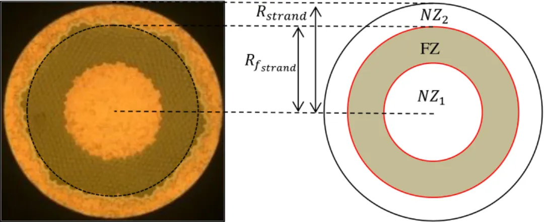
There are hundreds of strands in a CICC. The composites strands (cylindrical) are consisting of hundreds superconducting filaments (NbTi, Nb3Sn) twisted in a copper matrix with a twist pitch 𝑙_𝑝0 (as shown in

Figure 5). Filament diameter usually lies in the range of microns and they are usually located in what is known as the filamentary zone. Strands used in fusion machines are often composed of several layers, alternating resistive and filamentary zones. A resistive zone is mainly composed of copper and filamentary zone is mainly composed of twisted filaments of superconducting materials embedded in a normal matrix (see Figure 5). In this filamentary zone, we also find a resistive matrix usually made of copper filling every space between the filaments.

Architecture of the strand is different depending it is based on NbTi or Nb3Sn filaments. This is due to

the fact that Nb3Sn is issued from a chemical reaction taking place in the strand once it is produced.

Nb3Sn strands have to follow a peculiar thermal cycle to for the Nb3Sn phase to form in the strand. We

can see the different architectures in Figure 7.

Figure 5: Scheme of a superconducting strands on the left. Detailed architecture of JT-60SA TF conductor strand (0.81 mm diameter) on the right.

The strand itself can generate losses even though it is in its superconducting state. Subject either to external magnetic field or to current variations, it will generate losses of two kinds: hysteresis losses and coupling losses. Hysteresis losses are due to the current flowing inside the superconducting filaments whereas coupling losses are due to current crossing normal zone to connect two superconducting filaments. These currents, crossing normal zone in a strand, as depicted in Figure 6, are due to current redistribution inside the strand. This current redistribution is due to the fact that, in order to shield its volume from the external magnetic field variation, the twist of filaments in the strand will generate current loops. All these current loops together, limit the external field penetration into the strand filamentary zone by creating a magnetic field inside the strand, which is opposed to the external one.

These composite strands response to an external magnetic field variation is described by the following differential equation (1):

Figure 7: Different type of strands. NbTi (1st line) and Nb3Sn (2nd line). Extracted from [24].

Figure 6: Global current loops (in red) generated by applied field variation and generating coupling losses inside an example of composite strand.

𝐵𝑖+ 𝜏𝐵̇𝑖 = 𝐵𝑎 (1)

Where 𝐵𝑎 is the external field applied on the superconducting strand (or cable) and 𝐵𝑖 the internal field response to the applied one. 𝜏 is the time constant related to the current loop inside the strand.

This kind of currents generates, as described above, the so called coupling losses which are defined as:

𝑃_{𝑐𝑜𝑢𝑝𝑠𝑡𝑟𝑎𝑛𝑑} = 𝑛𝜏𝐵̇𝑖

2

𝜇0 (2)

where 𝑃𝑐𝑜𝑢𝑝_{𝑠𝑡𝑟𝑎𝑛𝑑} is the power per unit volume of strand with 𝑛 = 2 for a cylindrical composite. 𝑛 being a geometrical factor.

The relation between 𝐵𝑖 and 𝐵𝑎 can be illustrated for an applied sinusoidal field. If 𝐵𝑎= 𝐵𝑚sin(𝜔𝑡) + 𝐵𝑜𝑓𝑓, with 𝜔 = 2𝜋𝑓 the angular frequency, using the above first order differential equation (1), we obtain in complex notations:

𝐵̅𝑖=

𝐵𝑚𝑒𝑗𝜔𝑡

1 + 𝑗𝜔𝜏. (3)

Then we can readily give the internal magnetic field amplitude |𝐵̅𝑖| as:

|𝐵̅_𝑖| = 𝐵𝑚

√1 + (𝜔𝜏)2. (4)

The associated power density 𝑃_{𝑐𝑜𝑢𝑝𝑠𝑡𝑟𝑎𝑛𝑑} averaged over time (after a time long compared to 𝜏) will then be: 𝑃𝑐𝑜𝑢𝑝𝑠𝑡𝑟𝑎𝑛𝑑 = 𝐵𝑚2 2𝜇0 𝑛𝜏𝜔2 1 + (𝜔𝜏)2. (5)

As it is widely used within the applied superconductivity community, we can also express the losses in terms of average losses per cycle 𝑄 per unit volume (of strand), this can be done very quickly multiplying 𝑃 by the period 𝑇 of the cycle. Using the expression of 𝑃𝑐𝑜𝑢𝑝𝑠𝑡𝑟𝑎𝑛𝑑, we have:

𝑄_{𝑐𝑜𝑢𝑝𝑠𝑡𝑟𝑎𝑛𝑑} =𝐵𝑚

2 𝜇0

𝜋𝑛𝜏𝜔

1 + (𝜔𝜏)2. (6)

Of course, these considerations and formulae only concern the coupling losses generated by a strand subjected to a transverse field (as shown in Figure 6) and assume that the outer edge filaments are not saturated and that the composite is not carrying any transport current. In case of saturation, we would need to add the penetration losses, which are well described in [21].

I.4 Considerations on losses in superconducting magnets for fusion

Presently, several experimental superconducting tokamaks are in operation. The largest superconducting tokamak ever built (JT-60SA) is in its final phase of assembly and commissioning and first operation is expected end in 2020. The first plasma discharges of the superconducting experimental reactor (ITER) are expected in 2025. Moreover, studies are devoted to the design of reactors producing electricity after ITER (DEMO, DTT). On the energetic plan, fusion is obviously very attractive. The energy consumption of, for example, 400 000 inhabitants is in the range of 500 MW of electric power. In order to produce this amount of energy we would only need to burn 175 kg of deuterium tritium in a fusion plant while we would have used either 1.35 megatons of coal, or 0.9 megaton of petrol, or 12.5 tons of uranium in a fission plant. With renewable energy, it corresponds to 35 𝑘𝑚2 _{of solar panels or around} 25 𝑘𝑚2 of wind generator with a 20% load factor.

Using fusion plant instead of fission plant could offer nearly a carbon free electricity as fission but suppressing difficulties linked to fission as:

- Large available resources and suppression of the geopolitical tensions linked to fuel procurement.

- Simplification of the problems associated with long lived waste. - No uncontrolled chain reaction or runaway.

The demonstration of the feasibility of fusion was initiated in the eighties by the production of fusion power in JET and TFTR (see [22] and [23]). The operation of existing superconducting tokamak (WEST, EAST, KSTAR, etc.) is preparing ITER even if it was not their initial goal. The main objective of the ITER project, which will deliver first plasmas in 2025, is to demonstrate at a representative scale the feasibility of energy production using a fusion reactor under the form of a tokamak. The objective is to produce thousands of plasma discharges (500 MW during 500 s).

Applied Superconductivity in MRI is mainly in DC field. During ITER scenarios, causing large field variations across the magnets, important losses are developed associated to temperature increase and reduction of temperature margins. This is a new very important challenge for applied superconductivity. The ITER superconducting magnet system constitutes the largest ITER components, representing about 30% of the machine cost investment. This underlines the fact that designing the magnet system from specific design parameters in order to limit its AC losses remains a challenge. The objective is to keep the superconductors within their critical limits and to mitigate the power associated to the cryogenic system.

Since TORE SUPRA (CEA, Cadarache), now renamed WEST from its tungsten divertor upgrade, several other superconducting tokamaks are in operation. They are presented in Table 1 below:

Table 1: Superconducting fusion machines.

Starting from the first small superconducting magnet in 1962, unprecedented advances have been accomplished in applied superconductivity in particular in MRI. Regarding fusion, important challenges have been mastered such as the development of CICC to support very high currents (50-70 kA), very high voltage (10 kV), the description of AC losses generated by field variation and eliminated by the helium flowing inside the CICC. Connections of several superconducting coils have also been managed with the development of various connections techniques as the twin box developed at CEA Cadarache. In a CICC, strands are cabled and twisted in stages, and stages are also twisted and cabled as bigger stages. Regarding AC losses, the crucial role of the twist and transposition pitches is well known but the general impact of the geometry and in particular of the contact resistances between the cable strands has still to be explored. The cost investment of these large machines is dependent for a non-negligible part on the conductor itself. Progresses are needed to optimize and to analytically predict the behaviour of the CICCs under field variations.

Presently, the one time constant model is used in the fusion community to describe AC losses. Also numerical code (JackPot) or heuristic model (MPAS, for Multizone PArtial Shielding) exist but no analytical tools are capable of predicting the AC losses a CICC will generate with respect to its geometry, electrical contact distribution, and strand type. The objective of the thesis is to progress in this direction. Such a model presently exists at strand scale and it is named CLASS for Coupling Losses Algorithm for Superconducting Strand, developed by A. Louzguiti. This model (fully described in [24]) will be shortly introduced in Section II.1.2 for further uses. Based on this first step, he developed a two-stage cable model (see [24]) where two cabling two-stages of a CICC (example: the two first ones of JT-60SA TF conductor, a triplet of triplet) magnetically and electrically interact giving the amount of coupling losses generated by the coupling of two cabling stages.

The different versions of the conductors used in ITER are tested in the European SULTAN test facility (CRPP, see [25]). The test facility SULTAN inaugurated in 1992 in preparation of ITER has many objectives, among which:

- Critical properties characterisation of CICCs under representative magnetic field - Losses measurement in CICCs in harmonic field variations ranging from 0 to 10 Hz The experimental coupling losses are fitted using the heuristic MPAS model [26] (MPAS description will be done in Section II.1.1). The ITER scenarios are divided in small time steps into linear variations of magnetic fields, enabling to calculate the AC losses using the MPAS model and a model of hysteresis losses, then using a thermohydraulic code enables to check that the temperature margins are sufficient. This is the approach presently used in the ITER program to prepare the operation.

Machine Nature Nature R (m) 𝑩𝒎𝒂𝒙 (𝑻) TF system Stored Energy (MJ) TF system Sup Type/ 𝑻𝒐𝒑 (𝑲) Operation status

WEST Tokamak 2.4 9 600 NbTi/1.8 1988

LHD Heliotron 3.9 6.9 920 NbTi/5 1998

EAST Tokamak 1.7 5.8 400 NbTi/5 2006

KSTAR Tokamak 1.8 6.7 470 Nb3Sn

NbTi/5

2008

SST-1 Tokamak 1.1 4.2 56 NbTi/5 2008

W7-X Stellarator 5.5 5 620 NbTi/5 2015

JT-60SA Tokamak 3 5.65 1060 NbTi/5 Expected

2020

ITER Tokamak 6.2 11.8 40000 Nb3Sn

NbTi/5

Expected 2025

I.5 Thesis content and objectives

This thesis work aims at progressing in the analytical description of coupling losses under time varying field inside large superconducting cable in conduit conductors used for the magnet system of a fusion reactor. To illustrate this approach, the discussion about the presented models will be confronted to the modelling of cables of type similar to the TF conductor of JT-60SA.

The MPAS model (see [26]), which relies essentially on the experimental data of coupling losses gathered by using test facility as SULTAN, is used for ITER to assess the magnetic parameters of the considered cable. This model is not able to predict AC losses but only to give a description on how there are distributed in the cable among each stage. However, the present thesis is in line with the work led in [24], where an analytical model capable to model any two-stage cable was developed. We name this model COLISEUM for COupling Losses analytIcal Staged cablEs Unified Model. This modelling of a two-stage cable is not sufficient to properly model or predict the coupling losses generated by a cable composed with five stages for example. Further development toward higher number of stages has therefore been carried out within the thesis work.

Both of the above models are based on analytical expression of coupling losses but COLISEUM is intrinsically predictive as needing cable-oriented inputs as cable geometry and conductances between the cable stages. Based on the geometrical description of the cable (strand radius, twist pitches, cabling stage radius) and on its electrical description, COLISEUM can compute and tentatively predict induced current and coupling losses of a two-stage CICC (see [24]).

In its original state, COLISEUM could describe one-stage or two-stage cables but it has not been tested in a wide variety of parameters in order to check its consistency (check for divergence, limits of the model). We will start presenting briefly the CLASS model and the two versions of COLISEUM in their actual state (one-stage and two-stage description) for further use in the present work. MPAS will also be presented in two derived versions from its original formulation (see [26]) named restricted and advanced. Of course, these versions of heuristic model (MPAS) are developed to improve the unique time constant model which has shown some weaknesses in coupling losses description of CICC especially in fast transient regimes (see section II.1.1.1).

Using both CLASS and COLISEUM, we will first demonstrate the capability of the one-stage COLISEUM to reproduce the magnetic behaviour (time constant and shielding coefficient) of a strand modelled by CLASS. By using COLISEUM to replicate the strand from CLASS, we will be able to integrate the strand in the modelling of a two-stage cable. This first step will allow us to show an original analytical model for a composite strand as if coupled in multiplets.

The consistency of the two-stage COLISEUM is also tested to consolidate the validity of its description. Range and value of coupling parameters (time constants and shielding coefficients) with respect to cabling parameters (twist pitch, conductances), absence of divergences in the coupling parameters, correspondence with the one-stage COLISEUM are points that will be checked in order to be perfectly confident in the COLISEUM for its iteration to a 𝑛-stage description.

COLISEUM will be presented and discussed in its initial formulation and then simplified t its only relevant driving variables, already at the two-stage level, making it accessible to a fully explicit analytical approach and, further, prepare its extension to the description of cables with more than two

stages. The analytical extension of the COLISEUM will be managed and presented as well as some applicative cases to start exploring its predictive capability. Several demonstrations strengthen our modelling and are also discussed in this thesis work.

Also, various collaborations have been pursued during this thesis work. The first one was with INFLPR (RO) and I. Tiseanu on the study of tomographic images of CICC. This study led us to the analysis of the contact distribution of the CICC (JT-60SA TF type). We also started to develop an approach to reconstruct the contact network in the section of cable from tomographic images. Collaboration with the University of Twente has also been continued in the confrontation of both our model (COLISEUM and JackPot). This collaboration aims at confronting both models (JackPot and COLISEUM) in order for COLISEUM to strengthen the validity of its description.

The hypothesis in MPAS will also be discussed in order to provide this model sufficient degrees of freedom regarding the variety of cabling patterns existing among all CICCs.

During this thesis, several experimental campaigns have been led using CICC samples of the same type as the JT-60SA TF production cable. These measurements are led to benchmark our models and quantify the effect of the void fraction on coupling losses. The choice of JT-60SA TF is related to the fact that we have the samples ready to be used due to another previous experiment [27]. The outputs of the experimental campaigns we led during this thesis are twofold: on one side, we have explored and quantified the effect of various void fractions (different compaction rate) on the CICC sample AC performances. On the other side, we have started to constitute an experimental database in order to confront COLISEUM (once upgraded to an 𝑛-stage description) to the experimental data checking the validity of its predictions. A full description of the JOSEFA facility used to measure AC losses at CEA Cadarache will be given, with all the recent enhancements made on the facility to deliver a sinusoidal applied field. Several reminders will also be done regarding hysteresis and coupling losses modelling in order to describe the evaluation of AC losses from measured data.

The different measurements performed by using JOSEFA on the different versions of the JT-60SA TF conductor will allow us to confront the modelling given both by MPAS and an extended version of COLISEUM.

II.

Models

Content: This part is dedicated in a first time to the brief presentation of the four existing models developed at CEA:

- MPAS for cable.

- CLASS for composite strands.

- One-stage model to simulate one isolated cable stage named one-stage COLISEUM.

- Two-stage model to simulate the coupling between two consecutive cabling stages, named two-stage COLISEUM.

In a second time, applications of models (COLISEUM) are shown using JT-60SA TF cable parameters. Preliminary comments are given on both MPAS model and especially on COLISEUM regarding the handling and the outcome of the COLISEUM model at different scales of a cable (strand, one-stage and two-stage). We will demonstrate that the strand model and the two versions of COLISEUM (one-stage and two-stage) can be used at the same scale (i.e. strand scale), to model either a strand using the strand model or the one-stage COLISEUM or to model a multiplet of strand using the two-stage COLISEUM.

Then, based on those results, the first phase of our work is presented with, as preliminary step, a reduction of the dimension of the system equation describing the two-stage COLISEUM from dimension four to dimension two.

Associated publication:

M. Chiletti, J.L. Duchateau, F. Topin, B. Turck, L. Zani, “Analytical Modelling of CICCs

Coupling Losses: Broad Investigation of Two-Stage Model”, IEEE Trans. Appl. Superconductivity, Vol.

29, March 2019, Art. No. 4703005. [28]

II.1 Presentation of the models

II.1.1 The MPAS model

The MPAS model requires typically five couples of magnetic parameters to model the coupling experimental losses in a five-stage cable as a function of frequency: five time constants 𝜏 and five shielding coefficients 𝑛𝜅, one coupled (𝜏, 𝑛𝜅) per stage.

Using the initial description of the MPAS model in 2010 in [26], an effort was produced to reduce for the MPAS users the number of free parameters of the model to ease and rationalize the modelling work. This was done introducing an iterative process between magnetic parameters. Two models are given below to illustrate this effort especially applied on JT-60SA TF type cable (which is particularly homogeneous in pattern): the restricted MPAS and the advanced MPAS.

II.1.1.1 Restricted MPAS

The MPAS model (in its original formulation) is presently spreading within the fusion community. This model, in tight relation with AC losses characterization on samples, offers a method with a good compromise between simplicity and reliability to characterize AC coupling losses in the operation of large superconducting tokamaks. It has been shown (see [26]) that the classical model, with a unique time constant called “𝑛𝜏”, is not adequate to calculate losses for fast magnetic variations such as disruption, Vertical Displacement Event or even the initial discharge of the central solenoid (CS). MPAS was used for the first time for the estimation of the stability of JT-60SA TF conductor in case of a plasma disruption [26], [29]. MPAS has been applied for the estimation of the losses of the JT-60SA TF conductor [30]. For ITER, MPAS has been used as soon as 2013 in particular for the evaluation of AC losses in the ITER CS, for the reference 15 MA scenario [31]. Another application was the estimation of the Minimum Quench energy (MQE) of CS and PF ITER conductors [32]. It is now being used to estimate the losses of the CS Model coil under development in China within the CFETR reactor program [33].

The main advantage of the MPAS model lies in its simplicity, which makes its application straightforward, as soon as the AC coupling losses characterisation of the conductor is available out of a curve 𝑄(𝑓) obtained in experiments. The objective of this part of the thesis, in complement to the initial publication in Cryogenics [26], is to recall the bases of the MPAS model, and to detail some practical rules for the derivation of the model. Since 2010, substantial experience has been accumulated for characterisation of JT-60SA and ITER conductors. The resolution of some difficulties associated to this work will be discussed and illustrated along this thesis.

For a multistage cable, its behaviour is represented in MPAS by a given number of domains (typically the number of stages + the basic strand). Each domain is dominated by one stage in the cabling system. It can be represented by only two parameters: a time constant τ and a shielding coefficient 𝑛𝜅. These domains behave as dipoles. That means that, when submitted to an applied sinusoidal field 𝐵𝑎, an effective internal field 𝐵𝑖 is established, related to the external field by the linear differential equation (7):

𝐵𝑎 = 𝐵𝑖 + 𝜏 𝐵𝑖̇ .

(7)

That means also that, in each of these domains 𝑗, the coupling power loss per unit volume of cable can be calculated with the expression:

𝑃𝑗 =

𝑛𝜅𝑗𝜏𝑗 𝐵𝑖2̇ 𝜇0

₍₈₎

The total power dissipated in the cable is given by the sum of the contributions 𝑃𝑗 over the number of domains 𝑗. The modelling is usually made with shielding coefficients 𝑛𝜅𝑗 referring to the volume of superconducting strand rather than that of the whole cable. There is simply a factor 𝑟 =𝑆𝑐𝑎𝑏𝑙𝑒

𝑆𝑐𝑜𝑚𝑝 between

them, where 𝑆𝑐𝑎𝑏𝑙𝑒 and 𝑆𝑐𝑜𝑚𝑝 respectively stand for the circumscribed area of the cable and for the area of superconducting strand inside the cable. In the following, the parameters are therefore directly scaled

to the composite volume, in practical uses (such as comparisons with experiments) the results are referred to unit of volume of superconducting strand.

An iterative process is presented in details here to determine the relation between the coefficients 𝜅 as fully constrained. Some enhancements of the model are described in the following thesis. It is implicitly considered that the cable is homogeneous, which means that the transverse resistivity is average and constant inside the cable. Also, a first step of simplification is brought about: we reduce the number of degrees of freedom of the model to the minimum, i.e. one shielding coefficient and one time constant. This model is called the restricted MPAS.

𝜅𝑗 are the shielding coefficients in the volume of composites. Defining the last stage shielding coefficient 𝜅5, the other shielding coefficients are expressed by iteration as follows:

𝜅4= (1 − 𝜅5 2𝑟) 𝜅5 𝜅3= (1 − 𝜅5 2𝑟) 𝜅4= (1 − 𝜅5 2𝑟) 2 𝜅5 𝜅2= (1 − 𝜅5 2𝑟) 𝑘3 = (1 − 𝜅5 2𝑟) 3 𝜅5 𝜅1= (1 − 𝜅5 2𝑟) 𝑘2= (1 − 𝜅5 2𝑟) 4 𝜅5

The considered case is the one of a five-stage cable.

They can be iterated from the last stage shielding coefficient 𝜅5 as the only free parameters (for shielding coefficients) using the following relation (9):

𝜅𝑗−1

= (1 −

2𝑟

)

𝑜𝑟 𝑎𝑠

=

(1 −

2𝑟

)

We note that we can change the reference area of the shielding coefficients 𝜅𝑗 from the area of superconducting material to the circumscribed area of the cable (𝑘𝑗) expressed as follows:

𝜅𝑗= 𝑟 𝑘𝑗.

(10)

where 𝑟 =𝑆𝑐𝑎𝑏𝑙𝑒

𝑆_{𝑐𝑜𝑚𝑝}.

Regarding time constants 𝜏𝑗, they are proportional to the square of its twist pitch length 𝑙𝑝𝑗 as already

𝜏𝑗 = 𝛼 𝑙_𝑝𝑗2 𝜌𝑡 (11) 𝜏𝑗−1= 𝜏𝑗 [ 𝑙𝑝𝑗−1 𝑙𝑝𝑗 ] 2 (12)

with 𝛼 a constant coefficient.

We stress that this version of MPAS called restricted MPAS, using equations (9) and (12), is the version with the lowest number of degrees of freedom for this heuristic model, i.e. 𝜏5 and 𝑛𝜅5.

For their characterization, all ITER conductors have been tested in SULTAN facility in the range 0-10 Hz [25]. In the test facility, the conductor is submitted, in addition to the background magnetic field, to a sinusoidal perpendicular magnetic field excitation, such as: 𝐵⃗⃗⃗⃗ (𝑡) = 𝐵𝑎 𝑜𝑓𝑓𝑒⃗⃗⃗⃗ + 𝐵𝑥 𝑚𝑠𝑖𝑛(𝑡)𝑒⃗⃗⃗⃗ . Both 𝑦 magnetic fields are perpendicular and in addition transverse to the conductor (see Figure 8).

𝐵𝑜𝑓𝑓, the background field created by the test facility, stays constant during the AC loss experiment and it can be equal to 0.

At a given frequency (or corresponding ), the total volumetric losses (per volume of composite and per cycle) 𝑄𝑡𝑜𝑡 is measured. The experimental volumetric coupling losses 𝑄𝑐𝑜𝑢𝑝 is obtained by subtracting the hysteresis losses 𝑄ℎ𝑦𝑠𝑡. 𝑄ℎ𝑦𝑠𝑡must be calculated from the effective filament diameter 𝑑𝑒𝑓𝑓 and the critical properties of the current density ( 𝐽𝑐(𝐵𝑖, 𝑇) ) and not by extrapolation towards  = 0 of 𝑄𝑡𝑜𝑡 (the total losses), which is very imprecise. This operation can be delicate in particular in case of partial magnetic field penetration.

Figure 8: Respective orientation of pulsed field 𝐵𝑚 (red) created by the dipoles and background field 𝐵𝑜𝑓𝑓(blue) in SULTAN

test facility [25].

𝑥 𝑦

𝑄𝑐𝑜𝑢𝑝= 𝑄𝑡𝑜𝑡− 𝑄ℎ𝑦𝑠𝑡 (13)

In each cable domain 𝑗, the external applied field 𝐵𝑎 and the internal field 𝐵𝑖 associated with stage 𝑗: 𝐵𝑖𝑗, are linked by the following equation (14). Note that the internal field 𝐵𝑖𝑗 is different for each stage.

𝐵𝑖𝑗(𝑡) = 𝐵𝑎(𝑡) – 𝜏𝑗 𝐵̇𝑖𝑗 (14)

The coupling loss power per unit volume of composites for a given stage can be derived according to the following equation (15).

𝑃𝑗(𝑡) = 𝑛𝜅𝑗𝜏𝑗 𝐵̇𝑖𝑗2

𝜇0 (15)

For a sinusoidal field excitation, solving (14):

𝐵𝑖𝑗(𝑡) = 𝐵𝑚 √2𝜏_𝑗2+1 sin (𝜔𝑡 − δ) (16) With: tan (δ) =𝜏𝑗 (17)

Integrating 𝑃𝑗(𝑡) over a cycle for a given pulsation 𝜔 and a given stage 𝑗, gives the coupling energy per cycle and per unit volume of composite (from (15) and (16)):

𝑄𝑐𝑜𝑢𝑝_𝑗= 𝜅𝑗 𝐵𝑚2 ₀ 𝜏𝑗 (2_𝜏 𝑗2+ 1) . ₍₁₈₎

Considering all five stages of the conductor the total coupling losses QMPAS per cycle and per unit volume

of composite is:

𝑄𝑀𝑃𝐴𝑆(ω) = ∑ 𝑄𝑐𝑜𝑢𝑝𝑗(ω) 5

j=1

. (19)

Similarly, for comparison with equation (19), the energy associated with 𝜏𝑠𝑡 (𝜏 Single Time constant) given by using the model with the single time constant can be calculated as in [34]:

𝑛𝜏𝑠𝑡 = ∑ 𝜅𝑗𝜏𝑗 5 𝑗=1 (20) 𝑸𝒔𝒕 = 𝒏 𝑩𝒎𝟐 _𝟎 𝝉𝒔𝒕 (𝟐_𝝉 𝒔𝒕 𝟐 _{+ 𝟏)}. (21)

The use of a multi-constant model is necessary as the single time constant model (Q_ST in Figure 9) is less efficient to model the experimental coupling losses generated in a CICC at high frequency as shown in Figure 9 below:

Since its first development, MPAS has already evolved towards the above presented version (described with equations (9) and (12)) which is kind of a fully constrained MPAS.

During this thesis work, we will show that starting with a MPAS with the minimal number of free parameters and giving it more freedom by unrestricting one degree of freedom is a good option to fit coupling losses in a more general way than with the restricted MPAS.

0

5

10

15

20

25

30

35

40

0

1

2

3

4

Co

upling l

os

s

e

s

(mJ/

c

m3

/c

y

c

le

)

Frequency (Hz)

Q_MPAS

expSultan

Q_ST

Figure 9: Coupling losses for JT-60SA TF conductor in the frequency range (0-4 Hz) are represented with black dots. Resulting MPAS fit in blue and single time constant model in red (𝐵𝑜𝑓𝑓= 0 T left leg virgin 𝐵𝑚= 0.1 T).Data are Extracted from [59].

II.1.1.2 Advanced MPAS

The development of the MPAS in the original paper (see [26]), leads to quite general results. The only strong condition being that the basic time constants be well distant.

For the shielding coefficients, the cascade of shielding coefficients could be formulated with different basic shielding coefficient per stage based on recent results. As a matter of fact, it is evidenced in [24] that the shielding coefficient should be larger for a sextuplet than for a quadruplet or a triplet, for instance.

Based on the above result, our intuition to provide MPAS more flexibility (with respect to its restricted version) was to unconstraint some shielding coefficients by using the hypothesis that each stage can be composed of a different number of elements (i.e. DEMO, JT-60SA) which affect their shielding coefficient differently. For instance, in the JT-60SA TF conductor all stages are triplets except the last stage which is a sextuplet. We thus modify the iteration rules for shielding coefficients based on the above assumptions that this rule cannot be the same when going from a triplet to a triplet or from a sextuplet to a triplet for example. As said earlier, that affects the modelling of the coupling losses generated in the cable. Thus the first enhancement is under the form of considering two intermediate variables called 𝜅𝑎 and 𝜅𝑏 instead of the only one in the restricted MPAS (i.e. 𝜅5) . We recall that this index 5 refers to the fifth stage of the cable.

We have to note that 𝜅𝑎 in this enhanced version of MPAS is similar to 𝜅5 of the first version of MPAS, it represents the last stage shielding coefficient. 𝜅𝑏 , as said earlier, represents the new degree of freedom of this advanced MPAS. For the computation of the shielding coefficient for the advanced MPAS, we have: 𝜅5= 𝜅𝑎 𝜅4= 𝜅𝑏(1 − 𝜅𝑎 2𝑟) 𝜅3= 𝜅4(1 − 𝜅𝑏 2𝑟) = 𝜅𝑏(1 − 𝜅𝑎 2𝑟) (1 − 𝜅𝑏 2𝑟) 𝜅2 = 𝜅3(1 − 𝜅𝑏 2𝑟) = 𝜅𝑏(1 − 𝜅𝑎 2𝑟) (1 − 𝜅𝑏 2𝑟) 2 𝜅1= 𝜅2(1 − 𝜅𝑏 2𝑟) = 𝜅𝑏(1 − 𝜅𝑎 2𝑟) (1 − 𝜅𝑏 2𝑟) 3 .

Redefining the iteration rules between shielding coefficients, the expression can be written as follows for a five-stage cable:

𝜅𝑗= 𝜅𝑏(1 − 𝜅𝑎 2𝑟) (1 − 𝜅𝑏 2𝑟) 4−𝑗 (22)

Following our above intuitions and hypotheses, we have to note that the expression (22) of the shielding coefficients depends on the cabling pattern of the considered cases, the above expression corresponding to the one of the JT-60SA TF cable where the difference is introduce between the fourth and fifth stages.

It is important to note that if we consider 𝜅𝑎= 𝜅𝑏= 𝜅5, we found that the above equation (22) is equal to equation (9) used for the restricted MPAS. Thus, the advanced MPAS contains the restricted MPAS in its modelling.

The iteration rule on the time constants is conserved with the ratio of consecutive twist pitches only. For the time constants, the main dimensional factor was given to the basic twist pitch lengths. In the development of section II.1.1, MPAS considers that the only varying parameters in between two-stage is the twist pitch and thus that it is this twist pitch which drives the relation between time constants as exposed in section II.1.1. The interstage conductances (or average resistivity as considered in MPAS) are considered constant in the whole cable.

We can already distinguish two approaches for MPAS:

- the initial one, called restricted MPAS, where time constants are iteratively derived through the ratio of twist pitches and shielding coefficients through equation (9)

- the enhanced one, called advanced MPAS, where time constants are still derived through the ratio of twist pitches but shielding coefficient are now iteratively derived through equation (22). In the restricted MPAS, the only free parameters are the last stage time constant 𝜏5 and the last stage shielding coefficient 𝜅5 (index 5 refers to the fact that we consider a five-stage cable).

In the advanced MPAS, we have one more free parameters. We can set the last stage time constant 𝜏5 as in the restricted MPAS but shielding coefficients are set using 𝜅𝑎 and 𝜅𝑏.

In order to be efficient in the probing of experimental data with the two versions of the MPAS model we deal with, we have developed a statistical approach (and the associated numerical tool) to study the parametric behaviour of both MPAS models with respect to the experimental data we measure during the thesis work (chapter IV and V).

II.1.2 Coupling Losses Algorithm for Superconducting Strands (CLASS)

Starting from the basic element composing CICCs – strands -, we briefly present the Coupling Losses Algorithm for Superconducting Strand (CLASS), which is a fully analytical algorithm capable to predict the coupling losses in a composite strand (see Figure 10). The strand is designed as a layered composite alternating normal and superconducting zones. The analytical tools needed for the development of this model can be found in [24] and in [35]. Normal zones are mainly composed of copper and superconducting zones are composed of hundreds of superconducting filaments embedded in a matrix of normal metal (mainly copper) with a specific twist pitch. In some cases (as presented in Figure 10), a cupronickel barrier (CuNi) is implemented to limit coupling current between the resistive zones of the strands.

This model can be used to simulate several types of layered composite strands as can be seen in Figure 11:

Figure 11: Scheme of the generic cross-section geometry considered in CLASS. n layers of radius 𝑅 that can be either

normal or superconducting.

Figure 10: Detailed architecture of JT-60SA TF conductor strand (0.81mm diameter). Composed of NbTi superconducting filaments.

This model predicts as many time constants as edges of filamentary zones. These edges are the surfaces where the coupling currents carried by superconducting filaments flow. Each surface current flows with its own time constant and shielding coefficient (𝜏, 𝑛𝜅).

The time constants are related to the current loops taking place inside the superconducting strand subjected to an external magnetic excitation. These currents loops inside the strand create an internal magnetic field 𝐵𝑖 which shields the inner volume of the filamentary zone of the strand.

As shielding coefficient 𝑛𝜅 is related to the capability for the considered current loops (time constant 𝜏) to shield the inner volume. The parameters (𝜏, 𝑛𝜅) will be referred as magnetic parameters in the following.

Using this model several parameters are needed to solve the system of equations and evaluate these magnetic parameters, for example:

• 𝑅_𝑖 the radius of each zone starting from 𝑅1 to 𝑅𝑛. • Zone type: R for resistive and F for filamentary. • Filament twist pitch length inside the strand named 𝑙_𝑝0.

• The expression of the applied magnetic field 𝐵𝑎 (amplitude, frequency, phase). • Transverse resistivity of each layer 𝜌_𝑡𝑖.

𝜌𝑡_𝑖 is a homogenized variable and is used in the computation of the time constants 𝜏 and of the shielding coefficient of the strand 𝑛𝜅.

On top of that, several assumptions are used and recalled here: • Invariant system along z-axis.

• Applied magnetic field 𝐵_𝑎 is transverse and spatially uniform within the composite. • The composite does not carry any transport current 𝐼_𝑡 = 0.

• Superconducting filaments are not saturated 𝐸⃗⃗⃗⃗⃗ = 0⃗ . 𝑠 • Superconducting filaments are lightly twisted (2𝜋𝑅

𝑙𝑝 )

2 ≪ 1.

This approach is generalized and based on the previous analytical approach developed in [21] and is in agreement with the state of the art concerning a simple strand model. In fact, with this approach we are able to see that the single time constant approach for a strand is not realistic in cases where strands show several edges of filamentary zones. They would have as many time constants as the number of edges of filamentary zones.

Based on the same principle of multiple superconducting layers shielding the interior volume of the strand, the one-stage model named one-stage COLISEUM is developed (see [24]) using superconducting tubes twisted in tangency condition and interacting together to shield the cable stage. CLASS cannot be coupled to another stage in order to form multiplets of composite. We will see in the following section II.3.1, using CLASS and the stage COLISEUM presented below, that this one-stage model can be used to reproduce the strand behaviour and geometry. In the next sub-section, we will briefly present the one-stage COLISEUM in order to be able to use its equations and results in the following work.

II.1.3 One-stage COLISEUM

The one-stage COLISEUM is based on superconducting elements of radius 𝑅𝑒𝑙𝑒𝑚 (red superconducting tubes + outer normal shells) assembled together in tangency conditions with a specific twist pitch (𝑙𝑝) in order to form a cable stage. Superconducting elements (i.e. red superconducting tubes + outer normal shells) in this system can either represent a strand or a group of strands (as a petal (i.e. multiple strands twisted together in several cabling stages)) as seen in Figure 12. This model, developed in [24] and in [36], is capable to compute the induced currents 𝐼𝑘 in these superconducting tubes taking into account their electric and magnetic interactions when subjected to a transverse sinusoidal magnetic field 𝐵𝑎. It can also predict the AC losses generated by such a system.

The current 𝐼𝑘 = 𝐼 cos ( 2𝜋𝑧

𝑙𝑝 +

2𝜋(𝑘−1)

𝑁 ) , which flows on the red superconducting shell as depicted in Figure 12, with amplitude 𝐼 which is a function of time only driven by the following equation (23):

𝐼 + 𝜏𝐼̇ = 4𝜎𝑅𝑐sin ( 𝜋 𝑁) 2 (𝑙𝑝 2𝜋) 2 𝐵̇𝑎= 𝐼𝑒𝑥𝑡 (23)

This model has been described in detail by A. Louzguiti in his thesis [24]. Based on the definition of the vector potential of each element, it can provide the magnetic parameters (time constant 𝜏, partial shielding coefficient 𝑛𝜅) of a one-stage system of twist pitch 𝑙𝑝 , composed of 𝑁 superconducting elements of radius 𝑅𝑒𝑙𝑒𝑚, with a filamentary zone radius named 𝑅𝑓. All 𝑁 superconducting elements are twisted with the cabling radius 𝑅𝑐 (blue stripped line). Thus, the circumscribed area of the system is 𝑅𝑐𝑖𝑟𝑐= 𝑅𝑒𝑙𝑒𝑚+ 𝑅𝑐 (black stripped line). Between each element, the current flows from one element to another with a conductance 𝜎 named interstage conductance of the considered stage generating the so called coupling losses.

Here also, the time constant 𝜏 is related to current loops taking place in the one-stage model. The current loops related to one-stage of a CICC (as described by the one-stage COLISEUM) is also characterized

𝑅𝑐𝑖𝑟𝑐 𝑙𝑝

𝜎

𝑅𝑒𝑙𝑒𝑚

𝑅𝑐 𝑅𝑓

Figure 12: Illustration of two systems modelled with the one stage COLISEUM composed of 8 elements (on the left) and of 3 elements (triplet on the right) with brown filamentary zone. All variables are defined in the text below.

𝐼𝑘

by a shielding coefficient 𝑛𝜅 which can be seen as the capability for the considered cabling stage to shield its inner circumscribed volume from the applied field.

A geometrical factor named 𝛾𝐵𝑖𝑜𝑡𝑆𝑎𝑣𝑎𝑟𝑡 is also used in the computation of these magnetic parameters in order to take full account of the peculiar twisted geometry of the system. Its analytical expression is not reported here because of its complexity and can be found in [24].

Thus we have: 𝜏 = { 𝜎𝛾𝐵𝑖𝑜𝑡𝑆𝑎𝑣𝑎𝑟𝑡( 𝑙𝑝 2𝜋) 2 𝑓𝑜𝑟 𝑁 = 2 4𝜎𝛾𝐵𝑖𝑜𝑡𝑆𝑎𝑣𝑎𝑟𝑡sin2( 𝜋 𝑁) ( 𝑙𝑝 2𝜋) 2 𝑓𝑜𝑟 𝑁 ≥ 3 (24) and 𝑛𝜅 = { 𝜇0 𝛾𝐵𝑖𝑜𝑡𝑆𝑎𝑣𝑎𝑟𝑡𝜋 ( 𝑅𝑐 𝑅𝑐+ 𝑅𝑒𝑙𝑒𝑚 ) 2 [1 − 𝑠𝑖𝑛𝑐 (4𝜋𝑧 𝑙𝑝 )] 𝑓𝑜𝑟 𝑁 = 2 𝜇0𝑁 2𝛾𝐵𝑖𝑜𝑡𝑆𝑎𝑣𝑎𝑟𝑡𝜋 ( 𝑅𝑐 𝑅𝑐+ 𝑅𝑒𝑙𝑒𝑚 ) 2 𝑓𝑜𝑟 𝑁 ≥ 3 (25)

Using cable parameters (𝜎, 𝑅𝑐, 𝑒𝑡𝑐) to determine these magnetic parameters, we are able to quantify the coupling losses per circumscribed cable area 𝑄𝑣𝑜𝑙 generated in a single stage of CICC. This fully analytical model can be used either to predict coupling losses or to fit existing coupling losses data.

𝑃𝑣𝑜𝑙(𝑧) = 𝑛𝜅𝜏𝐵̇_𝑖2

𝜇0

(26)

The formulation of the one-stage COLISEUM is based on a solid analytical basis and it appears that major variables such as the power per unit volume (equation 26) can be expressed under a form as the one of MPAS. This is a strong result of [24] that we will use in the following of this work to construct an analytical 𝑛-stages model close to the MPAS initial intuition.

The above one-stage model can be used to model any stage of a cable as a homogenous uncoupled stage where we only consider inter-elements coupling losses at the considered stage. It is the simplest analytical model to simulate inter-elements coupling losses in one cable stage. This one-stage model will also be used in the following to model a superconducting composite strand. Modelling a strand with this homogenized one-stage model will allow us to model analytically multiplets of composites with the two-stage COLISEUM.

It is important to note that modelling analytically multiplets of strands has remained so far due to the difficulty of handling the analytical description.

II.1.4 Two-stage COLISEUM

II.1.4.1 Presentation

The two-stage COLISEUM is a determining enhancement of the one-stage model. It describes a two-stage system using the same analytical methodology as used for the development of the one-stage COLISEUM (see [24]). The analytical description and the calculations are quite hard to handle but the magnetic parameters (𝜏, 𝑛𝜅) of the two-stage system have been derived in [24] and in [37].

In Figure 13, index 1 refers to the substage parameters and index 2 refers to the super-stage parameters. 𝐼1 and 𝐼2 are the amplitudes of the currents 𝐼𝑘1𝑘2 circulating on the red superconducting shell

of the superconducting element 𝑘1 in the second stage 𝑘2 in Figure 13 and used to compute the coupling currents inside the system, 𝑅𝑒𝑙𝑒𝑚 and 𝑅𝑐𝑖𝑟𝑐 stand respectively for the radius of a superconducting element of the first stage and for the radius of the circumscribed circle of the system. The superconducting elements in this model are the same as in the one-stage COLISEUM, they are named superconducting elements of radius 𝑅𝑒𝑙𝑒𝑚 and composed with the red superconducting tubes plus an outer normal zone around.

𝑅𝑐𝑖𝑟𝑐= 𝑅𝑐₂+ 𝑅𝑐₁+ 𝑅𝑒𝑙𝑒𝑚 (27)

Initially, the derivation of the magnetic parameters of the two-stage COLISEUM presented in [24] led to an infinite number of time constants and shielding coefficient. It was nonetheless shown in [24] that it was possible to reduce them to only four without significant loss of information as the infinite matrix of time constants was strongly dominated by its diagonal and as only some spatial modes were initially excited (see [24] for a complete explanation of the reduction process). A study in purely inductive regime presented in [24] assessed the validity of this approach.

Figure 13: Scheme of a triplet of triplet, composed of three triplets at the sub stage level and 1 triplet at the super stage level.

𝑅𝑐1and 𝑅𝑐2 are respectively the cabling radius of the substage and of the super-stage.

𝑙𝑝2 𝑙𝑝1 𝜎1 𝜎2 𝑅𝑐2 𝑅𝑐₁ 𝑥 𝑦 𝑧 𝑅𝑐𝑖𝑟𝑐 𝑅𝑒𝑙𝑒𝑚 𝐼𝑘1𝑘2