Flatness-based constrained control and model-free control applications to quadrotors and cloud computing

HAL Id: tel-03214205

https://tel.archives-ouvertes.fr/tel-03214205

HAL is a multi-disciplinary open access archive for the deposit and dissemination of sci-entific research documents, whether they are pub-lished or not. The documents may come from teaching and research institutions in France or abroad, or from public or private research centers.

L’archive ouverte pluridisciplinaire HAL, est destinée au dépôt et à la diffusion de documents scientifiques de niveau recherche, publiés ou non, émanant des établissements d’enseignement et de recherche français ou étrangers, des laboratoires publics ou privés.

Maria Bekcheva

To cite this version:

Maria Bekcheva. Flatness-based constrained control and model-free control applications to quadro-tors and cloud computing. Automatic. Université Paris Saclay (COmUE), 2019. English. �NNT : 2019SACLS218�. �tel-03214205�

Flatness-based Constrained

Control and Model-Free Control

Applications to Quadrotors and

Cloud Computing

préparée à l’Université Paris-Sud École doctorale n°580 Sciences et technologies de l'information et de la communication (STIC)

Spécialité de doctorat: Automatique

Thèse présentée et soutenue à Gif-sur-Yvette, le 11/07/2019, par

Maria BEKCHEVA

Composition du Jury :

Silviu Iulian NICULESCU, Directeur de Recherche CNRS

Université Paris-Saclay – L2S Président

Emmanuel DELALEAU, Professeur des Universités

École nationale d’ingénieurs de Brest – Dépt. de Mécatronique Rapporteur

Didier THEILLIOL, Professeur des Universités

Université de Lorraine – CRAN Rapporteur

Mireille BAYART, Professeur des Universités

Université de Lille - CRISTAL Examinatrice

Michel FLIESS, Directeur de Recherche CNRS Emérite

Ecole Polytechnique -LIX Examinateur

Cédric JOIN, Professeur des Universités

Université de Lorraine – CRAN Examinateur

Hugues MOUNIER, Professeur des Universités

Université Paris-Sud (Université Paris-Saclay) – L2S Directeur de thèse

Luca GRECO, Maître de Conférences

Université Paris-Sud (Université Paris-Saclay) – L2S Co-Directeur de thèse

NNT : 2 0 1 9 S A C L S 2 1 8

Université Paris-Saclay

Espace Technologique / Immeuble Discovery

Model-Free Control Applications to

Quadrotors and Cloud Computing

Maria Bekcheva

Université Paris-Saclay

Université Paris-Sud

A thesis submitted for the degree of

PhD

Mes premiers remerciements sont adressés à mon directeur de thèse Hugues Mounier. Je lui suis très reconnaissante pour ces années, durant lesquelles il m’a guidée sur plusieurs sujets, m’a encouragée dans les moments de doute et m’a conseillée avec patience et pédagogie. Je remercie Hugues d’être un directeur tolérable avec un esprit moderne, libre et innovant. Ce fut un privilège de travailler avec lui. Je remercie également mon co-directeur Luca Greco pour ses précieux conseils, son aide et ses encouragements durant ces années de collaboration.

Je voudrais remercier Michel Fliess et Cédric Join. Cédric m’a guidée et encouragée durant ces deux dernières années. J’ai beaucoup appris à son contact et je tiens à le remercier très chaleureusement pour ses précieux conseils et bienveillance. Je remercie très chaleureusement Michel Fliess pour sa bonne humeur, et ses paroles toujours encourageantes. Ma recherche a été profondément influencée par ses travaux et on peut déceler cette influence tout au long de ce mémoire. Je suis très heureuse d’avoir pu bénéficier de ses lumières. Il m’a fait partager avec enthousiasme son ample culture scientifique et son expérience.

Je suis honorée d’avoir eu comme rapporteurs Emmanuel Delaleau et Didier Theilliol. Un grand merci pour leur relecture attentive de mon manuscrit, leurs suggestions et corrections avisées.

Je remercie Silviu Niculescu de m’avoir fait l’honneur de présider mon jury de thèse, et pour ses précieux conseils et son aide tout au long de ma thèse.

Je tiens aussi à remercier Mireille Bayart, qui a accepté d’examiner mon travail. J’aimerai remercier toute l’équipe de L2S et l’école doctorale STIC pour leurs aides et sympathies et tout particulièrement Gilles Duc pour ses conseils adminis-tratives et pédagogiques éclairés.

Je remercie mes collègues docteurs et doctorants de L2S. Ce fut un grand plaisir de vous connaître, de partager nos recherches et de vous retrouver autour des

Je remercie infiniment mes parents et mon frère Branko, pour leur soutien et amour.

Enfin, je voudrais exprimer toute ma gratitude à Alireza qui, jour après jour, partage mes joies et mes peines, me supporte, m’encourage, m’inspire, me conseille, m’aime.

Motivation

L’Automatique, avec son sous-domaine mathématique Théorie du Contrôle, étudie les propriétés et la commande des systèmes dynamiques en ingénierie. Chaque système contrôlé est composé de commandes (on dit aussi entrée ou contrôle) u, d’états x et de sorties y. L’objectif de la théorie du contrôle est de concevoir une commande de telle sorte que les états et les sorties atteignent un objectif défini. Les commandes agissent sur les états qui représentent habituellement la dynamique interne du système. Alors que les sorties représentant les composants mesurables, sont liés aux états. Lorsque la commande dépend uniquement de la mesure de sortie et que seule l’erreur entre la référence et la sortie mesurée est utilisée dans la conception, la commande est appelée une rétro-action (on dit aussi retour d’état ou feedback). La commande de rétroaction ou le cadre avec un degré-de-liberté échoue souvent pour les systèmes non linéaires, où il n’existe pas de solution globale asymptotiquement stable qui satisfait les contraintes du système (comme indiqué dans [95]).

Dans cette thèse, nous travaillons dans le cadre de la platitude différentielle ou le cadre avec deux degrés de liberté, qui est composé de deux parties : un générateur (ou une planification) des trajectoires et une commande de rétroaction pour réduire les erreurs dues aux perturbations et incertitudes. Les travaux de recherche de Fliess et de ses collègues [54–56] sur les systèmes différentiellement plats et leurs propriétés ont permis d’approfondir la compréhension du suivi de trajectoire par le paramétrage des trajectoires du système. Pour un système plat [55], tous les états et les entrées peuvent être paramétrés via une sortie plate et la planification de trajectoire est obtenue sans résoudre les équations différentielles. De plus, dans le cadre des systèmes plats, le comportement de chaque variable du système peut être facilement analysé. De ce point de vue, la conception de la commande peut donc être décomposée en deux étapes :

• Conception des trajectoires de référence pour les sorties plates. Des calculs hors ligne des commandes en boucle ouverte (feedforward).

Cette conception en deux étapes convient mieux qu’une commande classique de rétro-action (schéma de stabilisation) c’est-à-dire un cadre avec un degré de liberté. La première étape consiste à obtenir une solution du premier ordre au problème de suivi de trajectoire en tenant compte du modèle du système (comme dans un schéma classique de stabilisation pure). La deuxième étape est une étape de raffinement, où l’erreur entre les valeurs mesurées réelles et les références suivies sera beaucoup plus petite que dans le cas de la stabilisation pure. Le cadre avec deux degrés de liberté est une solution plus attrayante compte tenu de l’effort de calcul, de la complexité et de la stabilité. En outre, de nombreuses classes de systèmes non linéaires sont différentiellement plates [55], ce qui les rend plus faciles à analyser.

Cependant, lorsque les systèmes plats sont confrontés au problème de la commande

avec contraintes, il y a encore de grandes difficultés qui subsistent. Contraintes

Les contraintes sont présentes dans tous les systèmes contrôlés et peuvent avoir des effets néfastes sur la performance du système si elles ne sont pas prises en compte dans la conception de la commande. En général, les contraintes découlent des relations constitutives et physiques existantes entre les composants du système et son environnement de travail. Le plus souvent, les contraintes sont identifiées par des contraintes d’entrée, contraintes d’état et/ou contraintes de sortie :

• Contraintes d’entrée

Les contraintes d’entrée dépendent des contraintes de l’actionneur. L’actionneur (par exemple, moteur, vanne, interrupteur) est un composant mécanique qui

reçoit un signal de commande et une source d’énergie (par exemple, électricité, liquide, air), et convertit l’énergie du signal en mouvement ou force. Les actionneurs sont soumis à des saturations d’amplitude et de vitesse. Ils ne sont capables de fournir qu’une quantité limitée de mouvement ou de force. L’actionneur peut prendre une valeur entre une limite inférieure et supérieure

umin < u < umax. Dans certaines applications, les saturations sont évitées en choisissant des actionneurs plus puissants, mais cela peut ne pas être une solution permanente. Un exemple courant d’actionneur est le moteur à courant continu qui est présent dans chaque système de véhicule aérien sans pilote (UAV) pour fournir un mouvement de rotation. Le moteur à courant continu est limité en tension et en courant. D’autres exemples de contraintes d’entrée sont : le couple maximal disponible pour les dispositifs mécatroniques ou la puissance de refroidissement/chauffage limitée pour les réacteurs chimiques.

considérer les exemples suivants : dans les robots mobiles non-holonomes (par exemple, un chariot avec deux roues motrices avant et deux roues arrière qui ne peuvent pas se déplacer latéralement), les contraintes sur les vitesses longitudinales et angulaires; dans les systèmes sous-actionnés (par exemple, le quadrirotor), les contraintes sur les angles; dans les processus chimiques, les contraintes sur les variables du processus.

• Contraintes de sortie

Les contraintes de sortie sont généralement définies par l’environnement de travail. Dans la planification des mouvements, les robots mobiles se déplacent d’un point à l’autre tout en évitant les obstacles de l’environnement. Dans certaines applications, pour des raisons de sécurité ou de confort, des contraintes de sortie sont imposées par la demande des utilisateurs. Par exemple, limitations sur les vitesses longitudinales, les vitesses angulaires, les températures.

La trajectoire de référence doit tenir compte des contraintes du système. Une telle trajectoire qui se trouve à l’intérieur du domaine d’état admissible et qui respecte les contraintes s’appelle une trajectoire réalisable. Si les contraintes du système ne sont pas prises en compte, la trajectoire peut être irréalisable et la mission définie peut ne pas être accomplie. L’échec d’une mission se produit par exemple lorsque les actionneurs atteignent leurs limites et ne peuvent pas fournir les entrées d’actionnement souhaitées par le contrôleur.

Il est donc susceptible d’avoir un générateur de trajectoires qui définit un ensemble de trajectoires de référence réalisables c-à-d feed-forwarding trajectoires qui répondront aux contraintes définies. Une approche systématique capable de satisfaire les contraintes au préalable et d’intégrer la satisfaction des contraintes directement dans la formulation de la commande est un avantage clé. Ce fait nous motive à intégrer systématiquement les contraintes dans la conception de trajectoire.

Perturbations

Pour un système physique, à part la satisfaction des contraintes, le traitement des perturbations est essentiel à son bon fonctionnement. Par exemple, un quadrirotor devrait suivre sa trajectoire malgré les perturbations dues au vent ou la variation de masse (lorsqu’il transporte une charge). Cependant, lors de la compensation des perturbations, les trajectoires de référence dans le temps doivent induire un mouve-ment suffisammouve-ment lent, c’est-à-dire diminuer sa vitesse ou changer sa trajectoire de référence initiale afin d’éviter les saturations des moteurs du quadrirotor.

ce que les contraintes soient respectées. Dans la pratique de l’automatique, pour annuler les perturbations, un contrôleur en boucle fermée ou un contrôleur de

rétroaction est utilisé pour surmonter les limites du contrôleur en boucle ouverte.

Les perturbations du système peuvent être divisées en deux groupes :

• perturbations internes, par exemple, le modèle du système est inconnu ou en partie inconnu, les incertitudes des paramètres du modèle, et

• pertubations externes, par exemple, le bruit des capteurs, les rafales de vent ou toute autre perturbation de l’environnement.

Pour traiter les perturbations du système, dans cette thèse, nous utilisons la Commande sans modèle. La Commande sans modèle (CSM), présenté par Michel Fliess et Cédric Join [47, 48], a déjà prouvé sa puissance à travers un large éventail d’applications réussies[1, 49, 93, 96, 105] et même, avec des résultats expérimentaux [59, 60] où le modèle du système et ses perturbations sont inconnus. Les tentatives réussies pour une commande sans modèle non-linéaire et pour une commande sans modèle pour les systèmes à retard sont présentées dans [26, 106] et dans [37] respectivement. La première preuve détaillée de la stabilité de la commande sans modèle qui fournit des informations sur les paramètres de contrôle, a été donnée dans [35].

Organisation de la thèse et contributions

Cette thèse est consacrée à deux problèmes : le premier est la commande des systèmes différentiellement plats avec contraintes, et le second est l’application de la Commande sans modèle en utilisant sa robustesse par rapport aux dynamiques et pertubations non modélisées du système et de son environnement (voir Figure 1.1).

Le but ultime de ce projet de thèse est de montrer que les contraintes peuvent être satisfaites par les entrées c-à-d les feedforwarding nominales, et que les perturbations internes et externes peuvent être gérées par la Commande sans modèle. Puisque l’objectif derrière ces deux problèmes de contrôle (les contraintes et les perturbations), est essentiel pour presque tous les systèmes de contrôle, il est intéressant de noter à quel point peu de recherche est faite pour traiter simultanément ces deux problèmes. La difficulté vient de la nécessité de replanifier rapidement la partie feedforwarding lorsqu’une perturbation importante se produit, si la partie feedback augmente. Lorsque de telles perturbations se produisent, une replanification rapide de la trajectoire est essentielle pour éviter la saturation de l’actionneur. Dans [127] est présenté une commande composée de deux parties : la première partie est construite selon la platitude differentielle et la seconde partie suit la commande sans modèle pour un cas particulier où la perturbation et sa dérivée sont supposées bornées.

Pour ce faire, nous avons étudié la planification de trajectoire sous contraintes présentée dans la première partie de la thèse, où nous définissons un ensemble de trajectoires réalisables.

• Dans le chapitre 2, nous nous concentrons sur la génération de trajectoires réalisables plutôt que sur la stabilisation ou le feedback. Notre but est d’écrire les contraintes d’entrée et d’état en termes de la sortie plate et ses dérivés. Nous proposons d’utiliser les courbes de Bézier comme trajectoires de référence pour la sortie plate en raison de leurs propriétés utiles (une des clés dans la conception de notre contrôle en boucle ouverte sous contraintes). Nous montrons comment les entrées exprimées par les sorties plates, représentées chacune par une courbe de Bézier, peuvent être exprimées sous la forme d’une combinaison de courbes de Bézier. On obtient ainsi des équations explicites pour les points de contrôle d’entrée et d’état en fonction des points de contrôle des sorties plates. Nous recherchons ensuite les régions réalisables des points de contrôle de Bézier, c’est-à-dire un ensemble de trajectoires de référence réalisables. Il existe un certain nombre d’approches connexes [43, 62, 63, 79, 80, 120, 128, 129, 136] qui reposent toutes sur des procédures d’optimisation pour obtenir une trajectoire de référence réalisable. De plus, les systèmes différentiellement plats avec contraintes sont généralement attaqués en utilisant la commande optimale (voir, par exemple, [38, 42, 108, 111, 126]). • Dans le chapitre 3, nous étudions les systèmes avec des contraintes en

présence de retards sur l’état ou l’entrée. Une grande partie de la littérature d’automatique est consacrée à l’étude des systèmes linéaires et non linéaires avec des retards [119], mais peu de résultats sont capables de traiter les contraintes. Les contraintes sur l’entrée ou les variables d’état d’un système à retard sont généralement traitées avec des méthodes numériques impliquant le calcul d’intervalles invariants de trajectoire [103] et d’ensembles invariants positifs [32, 70], ou plus complexes, mais similaires dans leur esprit, les approches de la commande prédictive (voir par exemple [87, 107]). Dans le cadre des systèmes à retards, une approche systématique capable d’intégrer directement dans la formulation de la commande, la satisfaction des contraintes sur les entrées/états reste manquante.

La seconde partie de la thèse présente la Commande sans modèle (CSM) [48] qui estime et annule les perturbations et la dynamique inconnue du système en se basant sur une modélisation ultra-locale. L’apport de la deuxième partie de la thèse

• Dans le chapitre 4, nous proposons une commande qui évite les procédures de modélisation/identification du système de quadrirotor tout en restant robuste par rapport aux perturbations endogènes (la performance de contrôle est indépendante de tout changement de masse, inertie, effets gyroscopiques ou aérodynamiques) et exogènes (vent, bruit des mesures). Pour atteindre notre objectif, en se basant sur la structure en cascade du quadrirotor, nous divisons le système en sous-systèmes de position et d’attitude, chacun contrôlé par une

CSM indépendante de la dynamique du système. Ensuite, nous donnons des

résultats probants sur la stabilité pratique de la commande proposée. Nous validons notre approche de contrôle dans trois scénarios réalistes : en présence d’un bruit de mesure inconnu, avec des perturbations du vent variant dans le temps et des variations de masse inconnues.

• Dans le chapitre 5, nous utilisons la CSM pour contrôler l’élasticité horizontale d’un système Cloud Computing. Comparé aux algorithmes commerciaux de "mise à l’échelle automatique", notre approche facilement implémentable se comporte mieux, même avec de fortes fluctuations de charge de travail. Ceci est confirmé par des expérimentations sur le cloud public Amazon Web Services (AWS).

• Enfin, au chapitre 6, nous résumons les travaux de recherche de la thèse et nous proposons, dans une perspective, une commande de type « boîte grise » à l’aide des deux études présentées ci-dessus.

1 Introduction 1

1.1 Motivation . . . 1

1.1.1 Constraints . . . 2

1.1.2 Disturbances . . . 3

1.2 Thesis Organization and Contributions . . . 4

2 Constraints on Nonlinear Finite Dimensional Flat Systems 9 2.1 Chapter overview . . . 10

2.2 Differential flatness overview . . . 14

2.3 Problem statement: Trajectory constraints fulfilment . . . 15

2.3.1 General problem formulation . . . 15

2.3.2 Constraints in the flat output space . . . 16

2.3.3 Problem specialisation . . . 18

2.3.4 Closed-loop trajectory tracking . . . 20

2.4 Preliminaries on Symbolic Bézier trajectory . . . 21

2.4.1 Definition of the Bézier curve . . . 22

2.4.2 Bézier properties . . . 22

2.4.3 Quantitative envelopes for the Bézier curve . . . 24

2.4.4 Symbolic Bézier operations . . . 26

2.4.5 Bézier time derivatives . . . 27

2.5 Constrained feedforward trajectory procedure . . . 30

2.6 Feasible control points regions . . . 31

2.6.1 Cylindrical Algebraic Decomposition . . . 33

2.6.2 Approximations of Semialgebraic Sets . . . 35

2.7 Applications . . . 37

2.7.1 Longitudinal dynamics of a vehicle . . . 37

2.7.2 Quadrotor dynamics . . . 41

2.8 Closing remarks . . . 54

2.A Geometrical signification of the Bezier operations . . . 57

2.B Trajectory Continuity . . . 57

3 Constraints on Linear Flat Systems with Delays 61

3.1 Chapter Overview . . . 62

3.2 R-freeness for delay linear systems . . . 63

3.2.1 Algebraic setting and preliminaries . . . 64

3.3 Stabilization of the system . . . 65

3.4 B-splines preliminaries . . . 65

3.4.1 B-splines . . . 66

3.4.2 B-spline properties . . . 67

3.5 Constrained Trajectory Generation Procedure . . . 68

3.5.1 Derivative property of the B-spline curve . . . 68

3.5.2 Integral property of B-spline curve . . . 69

3.5.3 Degree elevation and knot insertion . . . 70

3.5.4 Reference trajectory design procedure . . . 70

3.6 Example: Car-following model . . . 71

3.7 Closing remarks . . . 74

4 Cascaded Model-Free Control of Quadrotors 77 4.1 Chapter overview . . . 79

4.2 Quadrotor model . . . 81

4.3 Control design . . . 83

4.3.1 Preliminaries for Model-Free Control . . . 83

4.3.2 Cascaded-model-free approach for the quadrotor . . . 85

4.3.3 Outer-loop Position control . . . 86

4.3.4 Inner-loop Attitude control . . . 87

4.4 Practical stability . . . 87

4.4.1 The system error dynamics . . . 88

4.5 Stability results . . . 89

4.6 Stability proof . . . 90

4.6.1 Position error subsystem . . . 91

4.6.2 Attitude error subsystem . . . 91

4.6.3 Verification of the assumptions . . . 91

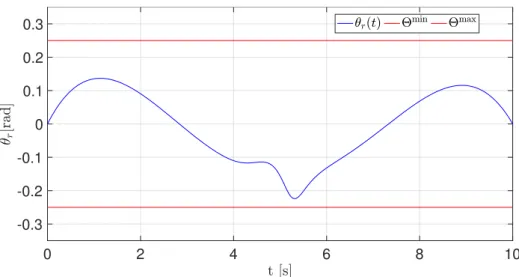
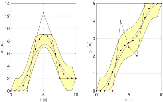
4.7 Aggressive trajectory tracking . . . 92

4.7.1 The Lissajous trajectory . . . 93

4.7.2 The B-spline trajectory . . . 94

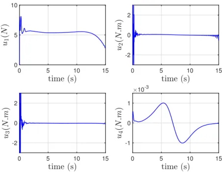
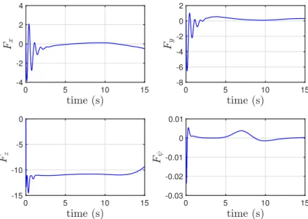
4.8 Simulation results . . . 96

4.8.1 Scenario 1: Unknown measurement noise . . . 97

4.8.2 Scenario 2: Unknown time-varying wind disturbance . . . . 100

4.8.3 Scenario 3: Mass parameter variation . . . 104

4.9 Closing remarks . . . 105

4.A Boundedness of the interconnection term . . . 109

5 Model-Free Control Framework for Cloud Resource Elasticity 113

5.1 Introduction . . . 114

5.1.1 Data is driving the revolution . . . 114

5.1.2 Utility Computing and Cloud Computing . . . 115

5.1.3 Problem statement . . . 116

5.2 Existing approaches . . . 119

5.3 Model-Free Control . . . 120

5.3.1 The ultra-local model . . . 120

5.3.2 Intelligent controllers . . . 121

5.3.3 Estimation of F . . . 121

5.4 Model-Free setting in the Cloud framework . . . 123

5.5 Experiments . . . 124

5.5.1 Experimental Setup . . . 126

5.5.2 Experimental results . . . 127

5.6 Closing remarks . . . 129

6 Conclusion and Future Works 135 6.1 Results summary and advantages . . . 135

6.2 Limits and further development tracks . . . 136

6.3 Future work: Robust control of flat systems . . . 137

1

Introduction

1.1 Motivation

Control System Engineering, together with its mathematical sub-field Control Theory, studies the properties of dynamical systems in engineering. Each control system is composed of inputs u, states x and outputs y. Control theory’s aim is to design a control input such that the states/outputs reach a defined goal. The inputs act on the states which usually represent the internal dynamics of the system. While the outputs representing the measurable components, are related to the states. When the control input solely depends on the output measure, and only the error between the reference goal and the measured output is used in the design, the control is called a feedback control. The feedback controller or the one-degree-of-freedom framework often fails for nonlinear systems, where a global asymptotically stable solution that satisfies the system constraints does not exist (as stated in [95]).

In this thesis, we work in the framework of differential flatness or the

two-degree-of-freedom framework, which is a combination of a trajectory generator and a

feedback controller. Fliess and his coworkers research work [54–56] on differentially flat systems and their properties led to a deeper understanding of trajectory tracking through the system trajectories parametrization. For a differentially flat system [55], all the states and the inputs can be parametrized through a so-called flat

output and the trajectory planning can be obtained immediately without solving

differential equations. Moreover, with the flatness property, the behaviour of each system variable can be easily analyzed. From this perspective, the control design can thus be decomposed in two steps:

• Design of flat outputs reference trajectory; off-line computation of the open-loop controls (feedforward part).

• On-line computation of the complementary closed-loop controls in order to stabilize the system around the reference trajectories (feedback part).

This two-step design is better suited than a classical feedback controller (stabilization scheme) i.e. one-degree of-freedom framework. The first step obtains a first-order solution to the tracking problem while following the model instead of forcing it (like in a usual pure stabilization scheme). The second step is a refinement one, where the error between the actual measured values and the tracked references will be much smaller than in the pure stabilization case. The two-degree-of-freedom framework is a more attractive solution considering the computational effort, tuning complexity and stability. In addition, many classes of nonlinear systems are differentially flat [55], which makes them easier to analyse.

However, when the flat systems are faced with the problem of constrained control, there are still great difficulties that remain.

1.1.1 Constraints

Constraints are present in all control systems and may lead in damaging effects on the system performance unless they are accounted in the control design. In general, constraints arise from the constitutive and physical relationships existing between the components of the control system, and its working environment. Most often constraints are identified as input, state and/or output constraints:

• Input constraints:

The inputs constraints depend on the actuator constraints. Actuator (for

e.g. , motors, valves, switches) is a mechanical component of a system that

receives a control signal and a source of energy (e.g. , electricity, liquid, air), and converts the signal energy into motion or force. Actuators are subject to magnitude and rate saturations. They are able to deliver only a limited amount of motion or force. The actuator can take a value between a lower and upper limit umin< u < umax. In some applications, the saturations are avoided by choosing more powerful actuators but this may not be a permanent solution. A common example of actuator is the DC motor which is present in every unmanned aerial vehicle (UAV) system to deliver a rotational motion. The DC motor is constrained in input voltage and current (which without load is equivalent to a velocity or acceleration). Other examples for input constraints are: maximum available torque for mechatronic devices or limited cooling/heating power for chemical reactors.

• State constraints:

State constraints may arise from the system’s structure. We can considered the following examples: in non-holonomic mobile robots (e.g. , a cart with two forward driving wheels and two back wheels that cannot move sideways), constraints on forward and angular velocities; in underactuated systems (e.g. , a quadrotor), constraints on the angles; in chemical processes, constraints on the process variables.

• Output constraints:

The output constraints are usually defined by the working environment. In motion planning, mobile robots steer from one point to another while avoiding the obstacles in the environment. In some applications, for safety or comfort reasons, output constraints are imposed by the user demand. For instance, limitations on the longitudinal velocities, angular velocities, temperatures. The reference trajectory should consider the system’s constraints. Such a trajectory that lies inside the admissible state domain and that does not violate the constraints is called a feasible trajectory. If system’s constraints are not considered, the trajectory may be infeasible and the defined task may not be accomplished. Task unaccomplishment occurs for example when actuators hit their limits, and cannot deliver the actuation inputs desired by the controller.

It is therefore likely to have a trajectory generator that defines a set of feasible reference trajectories i.e. feed-forwarding trajectories that will fulfil the defined constraints. A systematic approach able to satisfy the constraints beforehand and to embed the constraint satisfaction directly in the control formulation is a key advantage. This fact motivates us to embed systematically the constraints in the trajectory design based on the flatness property.

1.1.2 Disturbances

For a physical system, besides constraints fulfilments, dealing with uncertain disturbances is essential to its well functioning. For example, a quadrotor should track its trajectory despite the wind perturbations or mass variation (when carrying a payload). However, when compensating the disturbances, the reference trajectories in time must induce a sufficiently slow motion i.e. decreasing its velocity or change its initial reference trajectory in order to avoid saturations of the quadrotors motors.

Consequently, an important control problem is how to design the reference trajectory in the presence of disturbances such that the constraints are fulfilled. In

control engineering practice, to cancel the disturbances, a closed-loop controller or a feedback controller is used to overcome the limitations of the open-loop controller. Moreover, the so-called robust controllers are able to compensate for disturbances that may affect the nominal evolution of the system. The system disturbances may be divided in two groups:

• internal disturbances, for, e.g., unknown model or partly model mismatching, model parameter uncertainties, and

• external disturbances, for, e.g., sensor noise, wind gusts or any other environ-mental disturbance.

To deal with the system disturbances, in this thesis, we employ the Model-Free Control. The Model-Model-Free Control (MFC), introduced by Michel Fliess and Cédric Join [47, 48], already proved its power through a wide range of successful applications[1, 49, 93, 96, 105] and even, with experimental results [59, 60], where the system model and disturbances are unknown. Successful attempts for nonlinear MFC and for delay systems are presented in [26, 106] and in [37] respectively. The first detailed proof of stability of the MFC that provides insights to the tuning of the control parameters, was given in [35].

1.2 Thesis Organization and Contributions

This thesis is devoted to two problems: the first is the control of differentially flat systems with constraints, and the second is the application of the Model-Free Control using its robustness with respect to unmodelled dynamics and uncertainty of the system and its environment (see Figure 1.1).

Remark 1.1 Each thesis chapter is self-explanatory and contains all the necessary introduction and preliminaries to its presented contents. In this introduction, we define the main lines of thought which we explain in more details in the corresponding chapters.

The ultimate goal of this thesis project is to show that constraints can be fulfilled through the nominal feedforwarding inputs, and that internal and external disturbances can be managed by the MFC. Since the goal behind these two control problems (the constraints and the disturbances), are essential for almost every control system, it is interesting to note how little research is done in simultaneously dealing with these two problems. The difficulty arises from the need to quickly re-plan the feedforwarding part when a big disturbance occurs i.e. the feedback part

Chapter 1 Introduction

Chapter 5 Model-Free Control Framework for

Cloud Elasticity Model-Free Control Applications Chapter 6 Conclusion And Future Works Flatness-based Constrained Control Chapter 4 Cascaded Model-Free Control of Quadrotors Chapter 3 Constraints on Linear Flat Systems with Delays Chapter 2

Constraints on Nonlinear Finite Dimensional Flat

Systems

Figure 1.1: Organization of the thesis

increases. When such disturbances occur, a fast trajectory re-planning is essential to avoid actuator saturation. In [127], is discussed the control law composed of two parts: first part is constructed following differential flatness and second part is following the model-free control law for a special case where the disturbance and its derivative are assumed to be bounded.

But what happens when a big disturbance suddenly occurs? How to quickly re-plan a new reference trajectory ?

To that purpose, we studied the constrained trajectory approach presented in the first part of the thesis, where we define a set of feasible trajectories.

• In Chapter 2, we focus on trajectories generation rather than feedback transformations. Our goal is to write the state/input constraints in terms of

flat output and its derivatives. We propose to use Bézier curves as reference trajectories because of their useful properties (one of the keys in the design of our constrained open-loop control). We show how the inputs expressed by the flat outputs, each represented in terms of a Bézier curve, can be expressed as a combination of Bézier curves. We thus obtain explicit equations for the input/state control points as functions of the flat output control points. We then search for feasible regions of the Bézier control points i.e. a set of feasible reference trajectories. There are a number of existing related approaches [43, 62, 63, 79, 80, 120, 128, 129, 136], which all rely on optimization procedures to obtain a flat output reference trajectory. Moreover, differentially flat systems with constraints are generally attacked through the use of optimal control problems (see, e.g. [38, 42, 108, 111, 126])).

• In Chapter 3, we study the presence of delays in the state or the input that characterizes many natural as well as artificial systems. A large part of the control literature is thus devoted to the study of linear and nonlinear delay systems [119], but few results are able to handle constraints. Constraints in the input or the state variables of a delay system are usually tackled with numerical methods entailing the computation of trajectory invariant intervals [103] and positively invariant sets [32, 70], or more complex, but similar in spirit, Model Predictive Control approaches (see for instance [87, 107]). A systematic approach capable of embedding the constraint satisfaction directly in the control formulation is still lacking for delay systems.

The second part of the thesis presents the Model-Free Control framework [48] which estimates and cancels the unknown disturbances and/or unknown system dynamics. The contribution of the second part of the thesis lies in two applications of the Model-Free Control (MFC) of different nature:

• In Chapter 4, we propose a controller design that avoids the quadrotor’s system identification procedures while staying robust with respect to the endogenous (the control performance is independent of any mass change, inertia, gyroscopic or aerodynamic effects) and exogenous disturbances (wind, measurement noise). To reach our goal, based on the cascaded structure of a quadrotor, we divide the system into positional and attitude subsystems each controlled by an independent Model-Free controller of second-order dynamics. Then, we give proof results on the practical stability of the proposed control

design. We validate our control approach in three realistic scenarios: in presence of unknown measurement noise, with unknown time-varying wind disturbances and mass variation.

• In Chapter 5, we use Model-Free Control to control the “horizontal elasticity” of a Cloud Computing system. When compared to the commercial “Auto-Scaling” algorithms, our easily implementable approach behaves better, even with sharp workload fluctuations. This is confirmed by experiments on the Amazon Web Services (AWS) public cloud.

• Finally, in Chapter 6, we summarize the research work of the thesis and propose, as a perspective, a unified gray-box framework using the two above presented studies.

2

Constraints on Nonlinear Finite

Dimensional Flat Systems

Contents

2.1 Chapter overview . . . 10 2.2 Differential flatness overview . . . 14 2.3 Problem statement: Trajectory constraints fulfilment 15 2.3.1 General problem formulation . . . 15 2.3.2 Constraints in the flat output space . . . 16 2.3.3 Problem specialisation . . . 18 2.3.4 Closed-loop trajectory tracking . . . 20 2.4 Preliminaries on Symbolic Bézier trajectory . . . 21 2.4.1 Definition of the Bézier curve . . . 22 2.4.2 Bézier properties . . . 22 2.4.3 Quantitative envelopes for the Bézier curve . . . 24 2.4.4 Symbolic Bézier operations . . . 26 2.4.5 Bézier time derivatives . . . 27 2.5 Constrained feedforward trajectory procedure . . . 30 2.6 Feasible control points regions . . . 31 2.6.1 Cylindrical Algebraic Decomposition . . . 33 2.6.2 Approximations of Semialgebraic Sets . . . 35 2.7 Applications . . . 37 2.7.1 Longitudinal dynamics of a vehicle . . . 37 2.7.2 Quadrotor dynamics . . . 41 2.8 Closing remarks . . . 54 2.A Geometrical signification of the Bezier operations . . 57 2.B Trajectory Continuity . . . 57

Abstract: This chapter presents an approach to embed the input/state/output constraints in a unified manner into the trajectory design for differentially flat systems. To that purpose, we specialize the flat outputs (or the reference trajectories) as Bézier curves. Using the flatness property, the system’s inputs/states can be expressed as a combination of Bézier curved flat outputs and their derivatives. Consequently, we explicitly obtain the expressions of the control points of the inputs/states Bézier curves as a combination of the control points of the flat outputs. By applying desired constraints to the latter control points, we find the feasible regions for the output Bézier control points i.e. a set of feasible reference trajectories.

2.1 Chapter overview

Motivation

The control of nonlinear systems subject to state and input constraints is one of the major challenges in control theory. Traditionally, in the control theory literature, the reference trajectory to be tracked is specified in advance. Moreover for some applications, for instance, the quadrotor trajectory tracking, selecting the right trajectory in order to avoid obstacles while not damaging the actuators is of crucial importance.

In the last few decades, Model Predictive Control (MPC) [22, 89] has achieved a big success in dealing with constrained control systems. Model predictive control is a form of control in which the current control law is obtained by solving, at each sampling instant, a finite horizon open-loop optimal control problem, using the current state of the system as the initial state; the optimization yields an optimal control sequence and the first control in this sequence is applied to the system. It has been widely applied in petro-chemical and related industries where satisfaction of constraints is particularly important because efficiency demands operating points on or close to the boundary of the set of admissible states and controls.

The optimal control or MPC maximize or minimize a defined performance criterion chosen by the user. The optimal control techniques, even in the case without constraints are usually discontinuous, which makes them less robust and more dependent of the initial conditions. In practice, this means that the delay formulation renders the numerical computation of the optimal solutions difficult.

A large part of the literature working on constrained control problems is focused on optimal trajectory generation [42, 79]. These studies are trying to find feasible trajectories that optimize the performance following a specified criterion. Defining

y

yr

Stabilized System

Two degree of freedom control scheme

Flat System Stabilizing Feedback Feedforwarding Control yd ud u The chosen trajectory Online Update of the Regions

Symbolic Constrained Reference Management System Specification: - Flat Model - Input/State Constraints - Singularities Environment Changes (Example: new obstacles) Conditions (Feasible regions)

on the reference trajectory

Stage B Stage A

A1

A2

B1 B2

Figure 2.1: Two degrees of freedom control scheme overview

the right criterion to optimize may be a difficult problem in practice. Usually, in such cases, the feasible and the optimal trajectory are not too much different. For example, in the case of autonomous vehicles [76], due to the dynamics, limited curvature, and under-actuation, a vehicle often has few options for how it changes lines on highways or how it travels over the space immediately in front of it. Regarding the complexity of the problem, searching for a feasible trajectory is easier, especially in the case where we need real-time re-planning [68, 69]. Considering that the evolution of transistor technologies is reaching its limits, low-complexity controllers that can take the constraints into account are of considerable interest. The same remark is valid when the system has sensors with limited performance.

Research objective and contribution

In this chapter, we propose a novel trajectory-based framework to deal with system constraints. We are answering the following question:

Question 2.1 How to design a set of the reference trajectories (or the feed-forwarding trajectories) of a nonlinear system such that the input, state and/or output con-straints are fulfilled?

For that purpose, we divide the control problem in two stages (see Figure 2.1). Our objective will be to elaborate a constrained reference trajectory management (Stage A) which is meant to be applied to already pre-stabilized systems (Stage B).

Unlike other receding horizon approaches which attempt to solve stabilization, tracking, and constraint fulfilment at the same time, we assume that in Stage

B, a primal controller has already been designed to stabilize the system which

provide nice tracking properties in the absence of constraints. In stage B, we employ the two-degree of freedom design consisting of a constrained trajectory design (constrained feedfowarding) and a feedback control.

In Stage A, the constraints are embedded in the flat output trajectory design. Thus, our constrained trajectory generator defines a feasible open-loop reference trajectory satisfying the states and/or control constraints that a primal feedback

controller will track and stabilize around.

To construct Stage A we first take advantage of the differential flatness property which serves as a base to construct our method. The differential flatness property yields exact expressions for the state and input trajectories of the system through trajectories of a flat output and its derivatives without integrating any differential equation. The latter property allows us to map the state/input constraints into the flat output trajectory space.

Then, in our symbolic approach (stage A1), we assign a Bézier curve to each flat output where the parameter to be chosen are the so-called control points (yielding a finite number of variables on a finite time horizon) given in a symbolic form. This kind of representation naturally offers several algebraic operations like the sum, the difference and multiplication, and affords us to preserve the explicit functions structure without employing discrete numerical methods. The advantage to deal with the constraints symbolically, rather than numerically, lies in that the symbolic solution explicitly depends on the control points of the reference trajectory. This allows to study how the input or state trajectories are influenced by the reference trajectory.

We find symbolic conditions on the trajectory control points such that the states/inputs constraints are fulfilled.

We translate the state/input constraints into constraints on the reference trajectory control points and we wish to reduce the solution of the systems of equations/inequations into a simpler one. Ideally, we want to find the exact set of solutions i.e. the constrained subspace.

We explain how this symbolic constrained subspace representation can be used for constrained feedforwarding trajectory selection. The stage A2 can be done in two different ways.

• When a system should track a trajectory in a static known environment, then the exact set of feasible trajectories is found and the trajectory is fixed by our choice. If the system’s environment changes, we only need to re-evaluate the exact symbolic solution with new numerical values.

• When a system should track a trajectory in an unknown environment with

moving objects, then, whenever necessary, the reference design modifies the

reference supplied to a primal control system so as to enforce the fulfilment of the constraints. This second problem is not addressed in the thesis.

Our approach is not based on any kind of optimization nor does it need computations for a given numerical value at each sampling step. We determine a set of feasible trajectories through the system constrained environment that enable a controller to make quick real-time decisions. For systems with singularities, we can isolate the singularities of the system by considering them as additional constraints.

Existing Methods

• Considering actuator constraints based on the derivatives of the flat output (for instance, the jerk [58, 143], snap [91]) can be too conservative for some systems. The fact that a feasible reference trajectory is designed following the system model structure allows to choose a quite aggressive reference trajectory. • In contrast to [136], we characterize the whose set of viable reference

trajecto-ries which take the constraints into account.

• In [131], the problem of constrained trajectory planning of differentially flat systems is cast into a simple quadratic programming problem ensuing computational advantages by using the flatness property and the B-splines curve’s properties. They simplify the computation complexity by taking advantage of the B-spline minimal (resp. maximal) control point. The simplicity comes at the price of having only minimal (resp. maximal) constant constraints that eliminate the possible feasible trajectories and renders this approach conservative.

• In [63], an inversion-based design is presented, in which the transition task between two stationary set-points is solved as a two-point boundary value problem. In this approach, the trajectory is defined as polynomial where only the initial and final states can be fixed.

• The thesis of Bak [7] compared existing methods to constrained controller design (anti-windup, predictive control, nonlinear methods), and introduced a nonlinear gain scheduling approach to handle actuator constraints.

Outline

This chapter is organized as follows:

• In section 2.2, we recall the notions of differential flatness for finite dimensional systems.

• In section 2.3, we present our problem statement for the constraints fulfilment through the reference trajectory.

• In section 2.4, we detail the flat output parameterization given by the Bézier curve, and its properties.

• In section 2.5, we give the whole procedure in establishing reference trajectories for constrained open-loop control. We illustrate the procedure through two applications in section 2.7.

• In section 2.6, we present the two methods that we have used to compute the constrained set of feasible trajectories.

2.2 Differential flatness overview

The concept of differential flatness was introduced in [55, 56] for non-linear finite dimensional systems. By the means of differential flatness, a non-linear system can be seen as a controllable linear system through a dynamical feedback.

A model shall be described by a differential system as:

˙x = f(x, u) (2.1)

where x œ Rn denote the state variables and u œ Rm the input vector. Such a system is said to be flat if there exists a set of flat outputs (or linearizing outputs) (equal in number to the number of inputs) given by

y = h(x, u, ˙u, ..., u(r)) (2.2)

with r œ N such that the components of y œ Rm and all their derivatives are functionally independent and such that we can parametrize every solution (x, u) of (2.1) in some dense open set by means of the flat output y and its derivatives

up to a finite order q:

x= Â(y, ˙y, ..., y(q≠1)), (2.3a)

where (Â, ’) are smooth functions that give the trajectories of x and u as functions of the flat outputs and their time derivatives. The preceding expressions in (2.3), will be used to obtain the so called open-loop controls. The differential flatness found numerous applications, non-holonomic systems, among others (see [126] and the references therein).

In the context of feedforwarding trajectories, the “degree of continuity” or the smoothness of the reference trajectory (or curve) is one of the most important factors. The smoothness of a trajectory is measured by the number of its contin-uous derivatives. We give the definitions on the trajectory continuity when it is represented by a parametric curve in the Appendix 2.B.

2.3 Problem statement: Trajectory constraints

fulfilment

Notation

Given the scalar function z œ CŸ(R, R) and the number – œ N, we denote by zÈ–Í the tuple of derivatives of z up to the order – 6 Ÿ: zÈ–Í= z, ˙z, ¨z, . . . , z(–). Given the vector function v = (v1, . . . , vq), vi œ CŸ(R, R) and the tuple – = (–1, . . . , –q),

–i œ N, we denote by vÈ–Í the tuple of derivatives of each component vi of v up to its respective order –i 6 Ÿ: vÈ–Í= v1, . . . , v(–1 1), v2, . . . , v(–2 2), . . . , vq, . . . , vq(–q).

2.3.1 General problem formulation

Consider the nonlinear system

˙x(t) = f(x(t), u(t)) (2.4)

with state vector x = (x1, . . . , xn) and control input u = (u1, . . . , um), xi, uj œ

CŸ([0, +Œ), R) for a suitable Ÿ œ N. We assume the state, the input and their derivatives to be subject to both inequality and equality constraints of the form

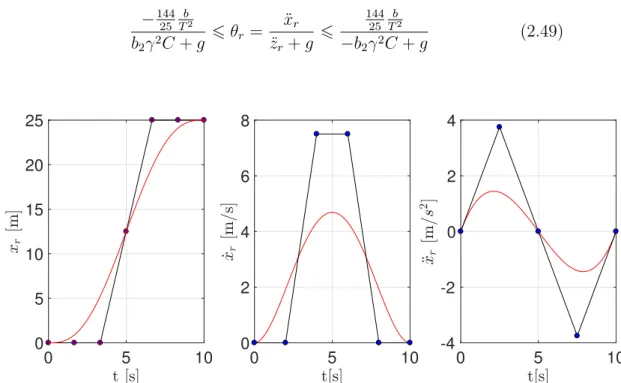
Ci(xÈ– x iÍ(t), uÈ–uiÍ(t)) 6 0 ’t œ [0, T ], ’i œ {1, . . . , ‹in} (2.5a) Dj(xÈ— x jÍ(t), uÈ—ujÍ(t)) = 0 ’t œ I j, ’j œ {1, . . . , ‹eq} (2.5b) with each Ij being either [0, T ] (continuous equality constraint) or a discrete set {t1, . . . , t“}, 0 Æ t1 6 · · · 6 t“ 6 T < +Œ (discrete equality constraint), and

–x

constraints) on the finite interval [0, T ]. Objectives can be also formulated as a concatenation of sub-objectives on a union of sub-intervals, provided that some continuity and/or regularity constraints are imposed on the boundaries of each sub-interval. Here we focus on just one of such intervals.

Our aim is to characterise the set of input and state trajectories (x, u) satisfying the system’s equations (2.4) and the constraints (2.5). More formally we state the following problem.

Problem 2.1 (Constrained trajectory set) Let C be a subspace of CŸ([0, +Œ), R).

Constructively characterise the set Ccons _{™ C}n+m of all extended trajectories (x, u)

satisfying the system (2.4) and the constraints (2.5).

Problem 2.1 can be considered as a generalisation of a constrained reachability problem (see for instance [43]). In such a reachability problem the stress is usually made on initial and final set-points and the goal is to find a suitable input to steer the state from the initial to the final point while possibly fulfilling the constraints. Here, we wish to give a functional characterisation of the overall set of extended trajectories (x, u) satisfying some given differential constraints. A classical constrained reachability problem can be cast in the present formalism by limiting the constraints Ci and Dj to x and u (and not their derivatives) and by forcing two of the equality constraints to coincide with the initial and final set-points.

Problem 2.1 is difficult to be addressed in its general setting. To simplify the problem, in the following we make some restrictions to the class of systems and to the functional space C . As a first assumption we limit the analysis to differentially flat systems [55].

2.3.2 Constraints in the flat output space

Let us assume that system (2.4) is differentially flat with flat output1

y = (y1, . . . , ym) = h(x, uÈfl u_Í

) , (2.6)

with flu _{œ N}m. Following Equation (2.3), the parameterisation or the feedforwarding trajectories associated to the reference trajectory yr is

xr = Â(yrÈ÷ x_Í ) (2.7a) ur = ’(yrÈ÷ u_Í ) , (2.7b)

with ÷x _{œ N}n and ÷u _{œ N}m.

Through the first step of the dynamical extension algorithm [44], we get the flat output dynamics

Y _ _ _ _ ] _ _ _ _ [ y₁(k1)= „₁(yȵy1Í_{, u}ȵu1Í) ... y(km) m = „m(yȵ y mÍ_{, u}ȵumÍ) , (2.8) with µy i = (µyi1, . . . , µyim) œ Nm, µui = (µiu1, . . . , µuim) œ Nm and ki > maxjµyji. The original n-dimensional dynamics (2.4) and the K-dimensional flat output dynamics (2.8) (K = q_iki) are in one-to-one correspondence through (2.6) and (2.7). Therefore, the constraints (2.5) can be re-written as

≈i(yrÈÊ in i Í) 6 0 ’t œ [0, T ], ’i œ {1, . . . , ‹in} (2.9a) ∆j(yrÈÊ eq j Í) = 0 ’t œ I j, ’j œ {1, . . . , ‹eq} (2.9b) with ≈i(yrÈÊ in i Í) = C_i((Â(y_rÈ÷xÍ))È–xiÍ, ’(y_rÈ÷uÍ)È–uiÍ), ∆j(yrÈÊ eq j Í) = D j((Â(yrÈ÷ x_Í )È—x jÍ, ’(y rÈ÷ u_Í )È—u jÍ) and Êin i , Êjeq œ Nm.

Remark 2.1 We may use the same result to embed an input rate constraint ˙ur.

Thus, Problem 2.1 can be transformed in terms of the flat output dynamics (2.8) and the constraints (2.9) as follows.

Problem 2.2 (Constrained flat output set) 2_{Let C}

ybe a subspace of Cp([0, +Œ), R)

with p = max((k1, . . . , km), Êin1, . . . , Ê‹inin, Êeq1 , . . . , Ê‹eqeq). Constructively characterise

the set Ccons

y ™ Cym of all flat outputs satisfying the dynamics (2.8) and the

constraints (2.9).

Working with differentially flat systems allows us to translate, in a unified fashion, all the state and input constraints as constraints in the flat outputs and their derivatives (See (2.9)). We remark that  and ’ in (2.7) are such that Â(yÈ÷xÍ)

and ’(yÈ÷uÍ) satisfy the dynamics of system (2.4) by construction. In other words,

the extended trajectories (x, u) of (2.4) are in one-to-one correspondence with

y _{œ C}m

y given by (2.6). Hence, choosing y solution of Problem 2.2 ensures that

x and u given by (2.7) are solutions of Problem 2.1.

2.3.3 Problem specialisation

For any practical purpose, one has to choose the functional space Cy to which all components of the flat output belong. Instead of making reference to the space Cgen:= Cp([0, +Œ), R), mentioned in the statement of Problem 2.1, we focus on the space Cgen

T := Cp([0, T ], R). Indeed, the constraints (2.9) specify finite-time objectives (and constraints) on the interval [0, T ]. Still, the problem exhibits an infinite dimensional complexity, whose reduction leads to choose an approximation space Capp _{that is dense in C}gen

T . A possible choice is to work with parametric functions expressed in terms of basis functions like, for instance, Bernstein-Bézier, Chebychev or Spline polynomials.

A scalar Bézier curve of degree N œ N in the Euclidean space R is defined as

P(s) =

N ÿ j=0

–jBjN(s), sœ [0, 1] where the –j œ R are the control points and BjN(s) =

1 N

j 2

(1 ≠ s)N≠j_sj are Bernstein polynomials [34]. For sake of simplicity, we set here T = 1 and we choose as functional space

Capp = I_N ÿ 0 –jBjN|N œ N, (–j)0N œ RN+1, Bj œ C0([0, 1], R) J (2.10) The set of Bézier functions of generic degree has the very useful property of being closed with respect to addition, multiplication, degree elevation, derivation and integration operations (see section 2.4). As a consequence, any polynomial integro-differential operator applied to a Bézier curve, still produces a Bézier curve (in general of different degree). Therefore, if the flat outputs y are chosen in Capp and the operators ≈i(·) and ∆j(·) in (2.9) are integro-differential polynomials, then such constraints can still be expressed in terms of Bézier curves in Capp_{. We stress} that, if some constraints do not admit such a description, we can still approximate them up to a prefixed precision Á as function in Capp _{by virtue of the denseness} of Capp _{in C}gen

1 . Hence we assume the following.

Assumption 2.1 Considering each flat output yrœ Capp defined as

yr = N ÿ j=0

the constraints (2.9) can be written as i(yrÈÊ in i Í) = N_iin ÿ k=0 ⁄ikBkN(s), (2.11) j(yrÈÊ eq j Í) = N_ieq ÿ k=0 ”jkBkN(s) (2.12) where ⁄ik = rinik(–0, . . . , –N) ”jk = reqjk(–0, . . . , –N) rin_ik, req_{jk œ R[–0}, . . . , –N] i.e. the ⁄ik and ”jk are polynomials in the –0, . . . , –N.⌅

Set the following expressions as‹in

rin = (rin_1,0, . . . , rin_‹in_,Nin ‹in), req = (req_1,0, . . . , req_‹eq_,Neq

‹eq), r= (rin, req),

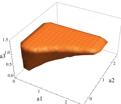
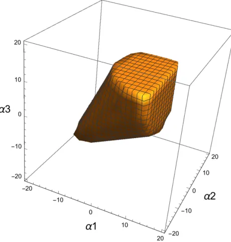
the control point vector – = (–1, . . . , –N), and the basis function vector B = (B1N, . . . , BN N). Therefore, we obtain a semi-algebraic set defined as:

I (r,A) =Ó–_{œ A | r}in(–) 6 0, req(–) = 0Ô

for any parallelotope

A = [–0,¯–0] ◊ · · · ◊ [–_N,¯–N], –i,¯–i œ R fi {≠Œ, Œ}, –i< ¯–i (2.13) Thus I (r, A) is a semi-algebraic set associated to the constraints (2.9). The parallelotope A represents the trajectory sheaf of available trajectories, among which the user is allowed to choose a reference. The semi-algebraic set I (r, A) represents how the set A is transformed in such a way that the trajectories fulfill the constraints (2.9). Then, picking an – in I (r, A) ensures that yr= –B automatically satisfies

the constraints (2.9).

The Problem 2.2 is then reformulated as :

Problem 2.3 For any fixed parallelotope A, constructively characterise the semi-algebraic set I (r, A).

This may be done through exact, symbolic techniques (such as, e.g. the Cylidrical Algebraic Decomposition) or through approximation techniques yielding outer approximations Iout

l (r, A) ´ I (r, A) and inner approximations Ilinn(r, A) ™ I (r,A) with lim læŒI out l = lim læŒI inn l = I . ⌅

This characterisation shall be useful to extract inner approximations of a special type yielding trajectory sheaves included in I (r, A). A specific example of this type of approximations will consist in disjoint unions of parallelotopes:

Ilinn(r, A) = € jœIl

Bl,j, ’i, j œ Il,Bl,ifl Bl,j = ÿ (2.14) This class of inner approximation is of practical importance for end users, as the applications in Section 2.7 illustrate.

2.3.4 Closed-loop trajectory tracking

So far this chapter has focused on the design of open-loop trajectories while assuming that the system model is perfectly known and that the initial conditions are exactly known. When the reference open-loop trajectories (xr, ur) are well-designed i.e.

respecting the constraints and avoiding the singularities, as discussed above, the system is close to the reference trajectory. However, to cope with the environmental disturbances and/or small model uncertainties, the tracking of the constrained open-loop trajectories should be made robust using feedback control. The feedback control guarantees the stability and a certain robustness of the approach, and is called the second degree of freedom of the primal controller (Stage B2 in figure 2.1). We recall that some flat systems can be transformed via endogenous feedback and coordinate change to a linear dynamics [55, 126]. To make this chapter self-contained, we briefly discuss the closed-loop trajectory tracking as presented in [88]. Consider a differentially flat system with flat output y = (y1, . . . , ym) (m being the number of independent inputs of the system). Let y_r(t) œ C÷(R) be a reference trajectory for y. Suppose the desired open-loop state/ input trajectories (xr(t), ur(t)) are generated offline. We need now a feedback control to track them.

Since the nominal open-loop control (or the feedforward input) linearizes the system, we can take a simple linear feedback, yielding the following closed-loop error dynamics:

e(÷)+ ⁄÷≠1e(÷≠1)+ · · · + ⁄1˙e + ⁄0e= 0 (2.15) where e = y ≠ yr is the tracking error and the coefficients = [⁄0, . . . , ⁄÷≠1] are chosen to ensure an asymptotically stable behaviour (see e.g. [56]).

Remark 2.2 Note that this is not true for all flat systems, in [66] can be found an example of flat system with nonlinear error dynamics.

Now let (x, u) be the closed-loop trajectories of the system. These variables can be expressed in terms of the flat output y as:

x= Â(yÈ÷≠1Í), u = ’(yÈ÷Í) (2.16)

Then, the associated reference open-loop trajectories (xr, ur) are given by

xr = Â(yrÈ÷≠1Í), ur = ’(yrÈ÷Í)

Therefore,

x= Â(yÈ÷≠1Í) = Â(yrÈ÷≠1Í+ eÈ÷≠1Í)

and

u= ’(yÈ÷Í) = ’(yrÈ÷Í+ eÈ÷Í,≠ eÈ÷Í).

As further demonstrated in [88][See Section 3.3], since the tracking error e æ 0 as t æ Œ that means x æ xr and u æ ur.

Besides the linear controller (Equation (2.15)), many different linear and non-linear feedback controls can be used to ensure convergence to zero of the tracking error. For instance, sliding mode control, high-gain control, passivity based control, model-free control, among others.

Remark 2.3 An alternative method to the feedback linearization, is the exact feedforward linearization presented in [67] where the problem of type "division by zero" in the control design is easily avoided. This control method removes the need for asymptotic observers since in its design the system states information is replaced by their corresponding reference trajectories. The robustness of the exact feedforwarding linearization was analyzed in [69].

2.4 Preliminaries on Symbolic Bézier trajectory

interpretations. The Bézier/B-spline curve can be handled by conveniently handling the curve’s control points.

The main reason in choosing the Bézier curves over the B-Splines curves, is the simplicity of their arithmetic operators presented further in this Section. Despite the nice local properties of the B-spline curve, the direct symbolic multiplication3 of B-splines lacks clarity and has partly known practical implementation [98].

In the following Section, we start by presenting the Bézier curve and its properties. Bézier curves are chosen to construct the reference trajectories because of their nice properties (smoothness, strong convex hull property, derivative property, arithmetic operations). They have their own type basis function, known as the Bernstein basis, which establishes a relationship with the so-called control polygon. A complete discussion about Bézier curves can be found in [116]. Here, some basic and key properties are recalled as a preliminary knowledge.

2.4.1 Definition of the Bézier curve

A Bézier curve is a parametric one that uses the Bernstein polynomials as a basis. An nth degree Bézier curve is defined by

f(t) =

N ÿ j=0

cjBj,N(t), 0 6 t 6 1 (2.17)

where the cj are the control points and the basis functions Bj,N(t) are the Bernstein

polynomials (see Figure 2.2). The Bj,N(t) can be obtained explicitly by:

Bj,N(t) = A N j B (1 ≠ t)N≠j_tj _{for j = 0, . . . , N.} or by recursion with the De Casteljau formula:

Bj,N(t) = (1 ≠ t)Bj,N≠1(t) + tBj≠1,N≠1(t).

2.4.2 Bézier properties

For the sake of completeness, we here list some important Bézier-Bernstein properties. 3_{The multiplication operator is essential when we want to work with polynomial systems.}

j= 2 j= 3 j= 4 j= 0 j= 1 0.0 0.2 0.4 0.6 0.8 1.0 0.0 0.2 0.4 0.6 0.8 1.0

Figure 2.2: Bernstein Basis for degree N = 4.

C4 C2

C0

Figure 2.3: The convex hull property for Bézier curve (N = 4) with control points