Holistic optimization of buildings based on the evaluation of annual performances from short simulation sequences

HAL Id: tel-03219964

https://tel.archives-ouvertes.fr/tel-03219964

HAL is a multi-disciplinary open access archive for the deposit and dissemination of sci-entific research documents, whether they are pub-lished or not. The documents may come from teaching and research institutions in France or abroad, or from public or private research centers.

L’archive ouverte pluridisciplinaire HAL, est destinée au dépôt et à la diffusion de documents scientifiques de niveau recherche, publiés ou non, émanant des établissements d’enseignement et de recherche français ou étrangers, des laboratoires publics ou privés.

evaluation of annual performances from short simulation

sequences

Hasan Sayegh

To cite this version:

Hasan Sayegh. Holistic optimization of buildings based on the evaluation of annual performances from short simulation sequences. Civil Engineering. Université savoie mont blanc, 2020. English. �tel-03219964�

THÈSE

Pour obtenir le grade de

DOCTEUR DE L’UNIVERSITÉ SAVOIE MONT

BLANC

Spécialité : Génie civil et sciences de l’habitat Arrêté ministériel : 25 Mai 2016

Présentée par

Hasan SAYEGH

Thèse dirigée par Gilles FRAISSE et Etienne WURTZ

encadrée par Antoine LECONTE et Simon ROUCHIER

préparée au sein du laboratoires LISE du CEA et LOCIE de l’Université Savoie Mont Blanc

dans l'École Doctorale SISEO

Holistic optimization of buildings

based on the evaluation of annual

performances from short simulation

sequences

Thèse soutenue publiquement le « 3 Décembre 2020 », devant le jury composé de :

Mrs, Evelyne, LUTTON

Directrice de recherche, INRAE, Président

Mr, Bruno, PEUPORTIER

Directeur de recherche, Ecole de Mines de Paris, Rapporteur,

Mr, Jean-Jacques, ROUX

Professeur, INSA Lyon, Rapporteur

Mr, Jean-Michel, RENEAUME

Professeur, Université de Pau et des pays de l’Adour, Examinateur

Mr, Gilles, FRAISSE

Professeur, Université Savoie Mont Blanc, Directeur de thèse

Mr, Etienne, WURTZ

Directeur de recherche, CEA, Codirecteur de thèse

Mr, Antoine, LECONTE

Docteur, CEA, Encadrant

Mr, Simon, ROUCHIER

iii

Abstract

Performing global approach studies on buildings, which take into consideration both the envelope and the connected systems, lead to the complexity of models under study. Simulation of such models may lead to high computational time expenses. Usually, simplified or surrogate models instead of detailed ones are used to avoid this issue. A global approach based on the reduction of input data profiles rather than the model itself is a current case of interest. The approach evaluates annual performances of a model starting from a short simulation sequence of typical selected days instead of complete data profiles.

After presenting and analyzing the methods used in the literature for typical day selection, the thesis presents a new iterative approach with an embedded grouping algorithm. The new algorithm, called TypSS (Typical Short Sequence) Algorithm, creates and enhances iteratively a short simulation sequence of typical days based on target criteria reflecting the annual performances of a model. The algorithm was applied on a detailed building model and led to much faster simulations while obtaining results of high correlation with the reference ones. Results were also compared to an iterative and a clustering approach used for day selection and its potential was noticed. The approach also showed its efficiency when generalized, and a sensitivity analysis on its input parameters was performed to evaluate its sensitivity to initial inputs imposed by operators.

Finally, the reduced sequence was used in a heavy multi-objective optimization study by NSGA-II. An adaptive strategy for optimization employing reduced sequences named OptiTypSS was introduced comparing the obtained results to an adaptive metamodel based approach. The method succeeded in obtaining optimal results very close to the ones from a reference full year simulation requiring less heavy simulations (30 for the metamodel approach while 9 for OptiTypSS). On the other hand computational time taken by the proposed strategy was higher than the one of metamodel due to the time consumed in the day selection process which could be enhanced in future work.

Keywords: Buildings, energy systems, short sequence, computation time reduction, multi-objective optimization.

v

Résumé

Les approches holistiques en modélisation des bâtiments sont des démarches globales considérant les fortes interactions entre l’enveloppe, les systèmes, l’environnement et les usagers. Par contre, ils sont très pénalisants en temps de calcul du fait de l’utilisation de modèles détaillés en régime dynamique et de périodes simulées longues. Dans ce contexte, la réduction du temps de calcul est un véritable défi pour les études holistiques.

La démarche classique utilise les méta-modèles ou des modèles réduits. La thèse explore une autre voie basée sur la réduction de la période simulée au lieu du modèle lui-même. L’objectif est de définir une séquence de jours suffisamment courte pour déterminer avec le modèle dynamique complet les performances qui sont ensuite extrapolées à l’année complète. Cela permettrait ainsi de développer une approche méthodologique plus rapide et plus accessible pour la conception des bâtiments. Après avoir présenté et analysé les méthodes utilisées dans la littérature, la thèse présente une nouvelle approche itérative intégrant un algorithme de regroupement. Le nouvel algorithme, appelé TypSS (Typique Short Sequence) Algorithme, crée et améliore de manière itérative une séquence courte de jours typiques basée sur des critères de sélection reflétant les performances annuelles d'un cas d’étude. L'algorithme a été appliqué sur un modèle de bâtiment détaillé et a conduit à des simulations beaucoup plus rapides tout en obtenant des résultats très proches des résultats annuels. Les résultats ont également été comparés à une approche itérative et de regroupement utilisées pour la sélection de jours et son potentiel a été remarqué. L'algorithme a également montré son efficacité lorsqu'elle est généralisée. Une analyse de sensibilité sur les paramètres d'entrée a été réalisée pour évaluer la sensibilité aux paramètres devant être fixés par un utilisateur.

Enfin, la séquence réduite a été utilisée dans une étude d'optimisation multicritères par NSGA-II. Une approche adaptative d'optimisation utilisant des séquences réduites nommée OptiTypSS est introduite en comparant les résultats obtenus à une approche adaptative basée sur le métamodèle. La méthode a permis d'obtenir des résultats très proches des individus optimaux obtenus à partir de simulations sur une année complète. D'autre part, le temps de calcul pris par la stratégie proposée était plus élevé

vi

que celui du métamodèle en raison du temps consommé dans le processus de sélection du jour. En conséquence, elle pourrait être amélioré dans les travaux futurs.

Mots clés: Bâtiments, systèmes énergétiques, séquence courte, réduction du temps de calcul, optimisation multi-objectifs.

vii

Acknowledgments

Three years of continuous work to be written in a single report was hard, but not as hard as writing this section. This path was full of great people that supported, encouraged and influenced me throughout this journey and I cannot mention them all in couple pages. To them all I dedicate this work.

I would like to acknowledge the financial support provided by the Region Auvergne-Rhône-Alpes, France for this PhD thesis through the project “Optimization of energy networks and energy producing buildings” OREBE. Thanks also to all partners contributing in the project for their interesting exchanges and valuable advices during the periodic meetings.

I would like to thank my directors and supervisors who were always around and assuring that I have all the necessary conditions to succeed. Gilles Fraisse for his excellent direction and all the time he dedicated for the success of this thesis throughout its course. Etienne Wurtz for the support, for believing in me, giving me the opportunity to participate in international projects and the efforts he did to assure the success of my international exchange program to Berkeley Lab. Antoine Leconte for his big heart and daily presence for all my questions making the long days of work go very smooth. And finally Simon Rouchier for his remarks regarding the coding and writing process.

I would like to thank every single colleague from CEA who became family after sharing a lot of good memories both in and outside the working hours. Special thanks go to Franck who was always a great support and helped me blend in since day one through his kind gestures and great humor. You were a huge part of this. Special thanks go also to Blaise and Clémence for always being kind and helping me fit better.

I would like to thank colleagues in LOCIE. From its director Monika Woloszyn to all permanent and non-permanent members and especially PhD students, we have shared a lot together. Special thanks go to Ainagul, Madina, Amin, Parul, Marie, Hugo and Gaetan, I am glad that we ended this journey as we started it, together. Thanks go also to Mathi, Manu and Taini for all the good memories we shared in and outside the lab.

viii

I would also like to thank colleagues from Berkeley lab for their kind welcome in my short yet very rich stay with them. Thanks to Michael, Jianjun, Kun, Nari, Tea, Haris, Lisa, Hagar, Antoine, Jose and Javi for the great time we spent. Thanks also to my roommates Arjit, Surej and Mohit. My American experience was unforgettable thanks to you all.

Thanks to all my Lebanese friends in France who were a great part of this journey. From Paris to Chambery you always made me feel home. I wish I could mention you all but you are too special to miss.

Finally I would like to thank my family. To my mom and dad who are the reason I made it so far. You have given me the light that I am following to pursue my dreams and for that I am forever thankful. Thanks to Ali, Hussein, Lamia and Youssef, my siblings and backbones whom I am blessed to have.

ix

Table of contents

Abstract --- iii

Résumé --- v

Acknowledgments --- vii

Table of contents --- ix

List of figures --- xiii

List of tables --- xvii

Abbreviations --- xix

Nomenclature --- xxi

General Introduction --- 1

Chapter I Concept of building performance evaluation and model

study by reduced sequences --- 3

I.1. Introduction --- 5

I.2. Buildings sector on worldwide scale --- 7

I.3. Buildings sector on French scale --- 8

I.4. Concept of building performance simulation (BPS) and optimization --- 9

I.5. Model study by short sequence --- 16

I.5.1. Heuristic Approaches --- 17

I.5.2. Iterative Approaches --- 18

I.5.3. Grouping Algorithms --- 19

I.6. Extrapolation of results --- 24

I.7. Analysis and discussion --- 24

I.8. Conclusion --- 28

Chapter II Description of the Typical Short Sequence algorithm

(TypSS) --- 31

II.1. Introduction --- 33

II.1.1. Objectives --- 33

II.1.2. Case study --- 33

II.2. TypSS: The process of the algorithm--- 37

II.2.1. Global Methodology --- 37

x

II.2.3. Initialization --- 42

II.2.4. Period setting phase--- 46

II.2.5. Typical days’ enhancement phase --- 52

II.3. Conclusion --- 58

Chapter III Application of TypSS and sensitivity analysis on its input

parameters --- 61

III.1. Introduction --- 63

III.2. Simulation results of the case study --- 64

III.2.1. Single individual I1 --- 64

III.2.1.1. Algorithm output --- 64

III.2.1.2. Temporal profiles of the target criteria --- 66

III.2.1.3. Annual values and cumulative profiles of the target criteria --- 69

III.2.1.4. Comparison with other approaches --- 72

III.2.2. Multiple tested individuals --- 77

III.2.2.1. Simulation results --- 77

III.3. Sensitivity of the TYPSS algorithm to its main parameters --- 81

III.3.1. Length of the initial sequence --- 83

III.3.2. Length of the generated sequence --- 85

III.3.3. Number of tested individuals --- 87

III.3.4. Number and type of the target criteria --- 91

III.4. Conclusion --- 96

Chapter IV Multi-objective optimization using reduced sequences:

Introducing OptiTypSS --- 99

IV.1. Introduction --- 101

IV.1.1. Objective --- 101

IV.1.2. Multi-objective optimization method --- 102

IV.1.3. Parametrizing the multi-objective optimization method --- 106

IV.2. Sequential multi-objective optimization methodology --- 109

IV.3. Adaptive multi-objective optimization methodology (OptiTypSS) --- 113

IV.4. Comparison of OptiTypSS with an adaptive metamodel based approach -- 119

IV.5. Conclusion --- 122

General conclusions and perspectives --- 125

xi

APPENDICES --- 147

Appendix A. Typical Short Sequence (TypSS) algorithm --- 149

Appendix B. Fifty samples generated by LHS --- 150

Appendix C. Temporal profiles obtained by reduced sequences of different

lengths --- 151

Appendix D. Periodic values obtained by reduced sequences of different

lengths --- 152

Appendix E. Cumulative profiles obtained by reduced sequences of different

lengths --- 153

Appendix F. CVRMSE influenced by the number of tested individuals -- 154

Appendix G. Two target criteria, three individuals Pareto front --- 154

Appendix H. Considering only three Pareto front individuals --- 155

Appendix I. Considering 10 individuals in OptiTypSS --- 156

xiii

List of figures

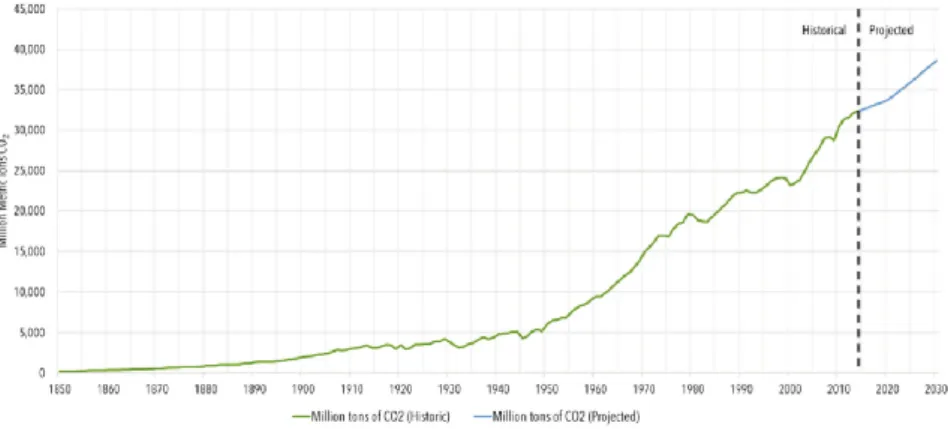
Figure I-1 . Evolution in global carbon dioxide emissions from 1850 to 2030. Source:

IEA. [8] --- 6

Figure I-2. Global final energy consumption by sector, history and projection. Source: IEA --- 6

Figure I-3. Final energy use per service in developed countries in 2007. Source: report of IIASA [10] (HDD = heating degree day). --- 7

Figure I-4. World final energy consumption by source in residential sectors (left), commercial and public (right) in 2007 [10] --- 7

Figure I-5. Final energy use for each sector adapted from French Environmental Energy Agency ADEME (Source: D. Mauree, 2014) --- 8

Figure I-6. Final energy use inside buildings adapted from French Environmental Energy Agency ADEME (Image credit: D. Mauree, 2014) --- 8

Figure I-7. The relation between the complexity of the case study and the type of time sequence used for simulations. --- 15

Figure I-8. General schema of the short sequence selection process followed by the iterative reduction approach. --- 17

Figure I-9. Heuristic method in typical day selection. --- 18

Figure I-10. Iterative method in typical day selection. --- 19

Figure I-11. Grouping method in typical day selection. --- 19

Figure I-12. Classification of clustering techniques [81] --- 20

Figure I-13. Principle of partitional and hierarchical clustering [82] --- 20

Figure I-14. Distribution of the reduction approaches as found in the literature.--- 25

Figure I-15. Approximation of the duration curves using the OPT approach to select a varying number of representative days [80] --- 25

Figure I-16. Approximation of the duration curves for two representative days selected by the different approaches [80] --- 25

Figure I-17. Relative error for the case of CHP system [82] --- 26

Figure I-18. Relative error for the case of residential system based on heat pumps and photovoltaics [82] --- 26

Figure II-1. A general scheme of a building model. --- 34

Figure II-2. Case study: (Up) solar combisystem connected to a building, (bottom) envelope parts with inside and outside facade areas. --- 35

Figure II-3. Daily (Left) and cumulative (Right) profiles of the target criteria: (a) backup energy, (b) energy stored in the tank, (c) internal room temperature. --- 36

xiv

Figure II-4. The global scheme of the algorithm TypSS. --- 38

Figure II-5. Fifty individual samples I50 found by Latin Hypercube Sampling. --- 41

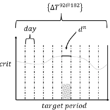
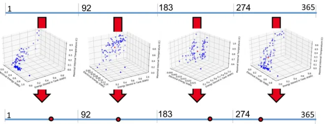
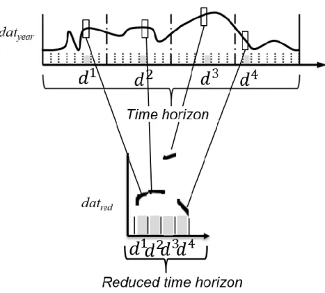
Figure II-6. Schema of a profile and dividing the year Tsim into four initial periods. - 42 Figure II-7. Profile of a criterion in period ∆T92@182 showing the day distribution in the period and a characteristic day dn. --- 43

Figure II-8. The process of generating the initial sequence of four days. --- 44

Figure II-9. The process of generating the reduced profile of the initial sequence starting from the annual one. --- 45

Figure II-10. The general process of the initialization phase. --- 45

Figure II-11. The general process of the Period setting phase. --- 46

Figure II-12. Comparison between the annual and extrapolated short sequence values for each criteria after being normalized and detecting the worst performing period (period 2). --- 51

Figure II-13. The process of detecting and dividing the worst performing period. --- 52

Figure II-14. The general process of the Typical days’ enhancement phase. --- 53

Figure II-15. The process of target period day modification. --- 56

Figure II-16. Scatter of the tested sequences (blue) with respect to the global coefficient of determination RGlobal2 and the global annual sum error EGlobal and the selected sequence (orange). --- 57

Figure III-1. The hourly ambient temperature and global horizontal radiation profiles: (a) reference annual profile (in blue) and the 12 selected days (in orange), (b) 12 selected days profile. --- 66

Figure III-2. Comparison between reference and extrapolated predicted backup energy: (a) temporal daily profile, (b) integrated values per period. --- 67

Figure III-3. Comparison between reference and extrapolated predicted energy stored in the tank: (a) temporal daily profile,( b) integrated values per period. --- 68

Figure III-4. Comparison between reference and predicted internal room temperature: (a) temporal daily profile, (b) averaged values per period. --- 69

Figure III-5. Annual and extrapolated cumulative profiles of the target criteria: (a) integrated backup energy, (b) integrated energy stored in the tank, (c) integrated internal room temperature. --- 70

Figure III-6. Principle of partitional clustering, Kotzur et al.[82] --- 73

Figure III-7. Annual and extrapolated cumulative profiles as obtained by the three methods: (a) backup energy, (b) energy stored in the tank, (c) internal room temperature. --- 77

Figure III-8. Annual (solid) and extrapolated cumulative (dashed) profiles as obtained by the five individuals: (a) backup energy, (b) energy stored in the tank, (c) internal room temperature. --- 79

xv

Figure III-9. Annual sum errors of the target criteria of all 50 individuals obtained after simulation with the typical day sequences obtained with one individual (orange) and five individuals (blue). --- 81 Figure III-10. Performances of generated sequences by TypSS starting from different initial sequences regarding each target criterion: (a) coefficient of determination, (b) annual sum error, (c) CVRMSE. --- 84 Figure III-11. Performances of generated sequences by TypSS of different sizes regarding each target criterion: (a) coefficient of determination, (b) annual sum error, (c) CVRMSE. --- 86 Figure III-12. Time recorded by the algorithm to converge to its final sequences of different sizes. --- 87 Figure III-13. Time recorded by the algorithm to converge to its final 12 days sequenc regarding different number of tested individuals. --- 88 Figure III-14. Global coefficient of determination recorded applying the generated sequences on their corresponding individuals (blue) and original 50 individuals (orange). --- 89 Figure III-15. Maximum annual sum errors recorded for each target criterion applying the generated sequences on: (a) their corresponding individuals and (b) the original 50 individuals. --- 90 Figure III-16. Cumulative profiles as obtained with different criteria combination: (a) backup energy, (b) energy stored in the tank, (c) internal room temperature. --- 93 Figure III-17. Annual sum errors of the target criteria of all 50 individuals obtained after simulation with the typical day sequences obtained with one criterion (blue), two criteria (orange) and three criteria (grey). --- 95 Figure IV-1. Dominated and Non-dominated regions of a reference point [96]. --- 103 Figure IV-2. Representation of the “crowding” distance [96]. --- 104 Figure IV-3. Example of a selection tournament for K = 3 and a maximization problem [97]. --- 105 Figure IV-4. Process of cross over between two parents and the mutation of a gene in their obtained child. --- 106 Figure IV-5. Reference Pareto front obtained with an annual simulation. --- 109 Figure IV-6. Predicted Pareto front with respect to the reference one after applying the short sequence obtained from a single individual and three target criteria. --- 109 Figure IV-7. Comparison between the reference and the two predicted Pareto fronts after applying the short sequence obtained from a single (blue) and five individuals (red) considering three target criteria. --- 111 Figure IV-8. Predicted Pareto front with respect to the reference one after applying the short sequence obtained from five individuals and backup energy as the only target criterion. --- 112

xvi

Figure IV-9. Proposed adaptive strategy to enhance the predicted Pareto front (OptiTypSS). --- 113 Figure IV-10. Predicted Pareto front obtained from three individuals and a single target criterion. Pareto is divided into three parts showing the initial and selected individuals. --- 115 Figure IV-11. Predicted Pareto front with respect to the reference one after applying the short sequence obtained from three individuals and a single target criterion.--- 116 Figure IV-12. Predicted Pareto front obtained from six individuals and a single target criterion. Pareto is divided into three parts showing the initial and selected individuals. --- 117 Figure IV-13. Predicted Pareto front with respect to the reference one after applying the proposed strategy. --- 118 Figure IV-14. Individuals corresponding the predicted (orange) and reference (blue) Pareto fronts as found after applying the proposed strategy. --- 119 Figure IV-15. The reference Pareto front with respect to the predicted ones by the proposed strategy and metamodel. --- 122

xvii

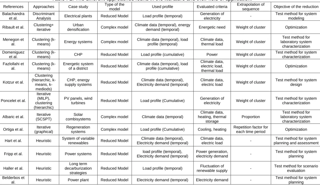
List of tables

Table I-1. The approaches used to reduce computational time expenses and their pros and cons. --- 16 Table I-2. The different approaches found in the literature and their field of application. --- 23 Table I-3. Comparison of the approaches --- 27 Table II-1. The parametric characteristics of the five initial individuals. --- 41 Table III-1.Typical short sequence of 12 days and the number of days in each period. --- 65 Table III-2. Comparison between reference and predicted annual sum of the target criteria. --- 72 Table III-3. Comparison between the three time reduction methods results. --- 75 Table III-4.Typical short sequence of 12 days and the number of days in each period obtained on five individuals. --- 77 Table III-5. The global and individual coefficient of determination of the three target criteria. --- 79 Table III-6. The reference (AN) and predicted (TS) annual values and their relative errors of the target criteria per individual. --- 80 Table III-7. Considered criteria in each case. --- 92 Table III-8. Results obtained with different criteria combination: considered criteria (in bold) and not considered criteria (italic). --- 93 Table III-9. Initial periods’ division influenced by the modification of the target criteria. --- 94 Table IV-1. Comparison between annual and predicted sums of the initial and selected individuals from the first predicted Pareto front. --- 116 Table IV-2. Comparison between annual and predicted sums of the initial and selected individuals from the second predicted Pareto front. --- 117 Table IV-3. Time consumed to obtain the final Pareto fronts of Reference, OptiTypSS and metamodel simulations. --- 121

xix

Abbreviations

ANN Artificial Neural Network

ASHRAE American Society of Heating, Refrigerating and Air-Conditioning Engineers

BES Building Energy Simulation BIM Building Information Modeling BOP Building Optimization Problem BPS Building Performance Simulation

CEA French Alternative Energies and Atomic Energy Commission

CHP Combined Heat and Power

CVRMSE Coefficient of Variation of Root Mean Square Error CO2 Carbon dioxide

DHW Domestic Hot Water GHG Greenhouse Gas HDD Heating Degree Day

IIASA International Institute for Applied Systems Analysis IPCC Intergovernmental Panel on Climate Change

LHS Latin Hypercube Sampling

MILP Mixed Integer Linear Programing NMBE Normalized Mean Bias Error

xx

NSGA-II Improved Non Dominated Sorting Genetic Algorithm OECD Organization for Economic Co-operation and

Development

OptiTypSS Strategy for multi-objective optimization with TypSS PSO Particle Swarm Optimization

RMSE Root-mean square error

SCSPT Short Cycle System Performance Test TypSS Typical Short Sequence Algorithm

xxi

Nomenclature

Variables

Used in model

INS Insulation thickness m

VST Volume of storage tank m3

SCOLL Surface of solar collector m²

Used in TypSS

𝑐𝑟𝑖𝑡 target criterion -

𝑐𝑟𝑖𝑡𝑦𝑒𝑎𝑟,𝑖𝑛𝑑𝑣𝑛,𝑗 Criterion value obtained with the reference annual

simulation for day j of the period n by the individual indv

criterion unit

𝑐𝑟𝑖𝑡_{𝑦𝑒𝑎𝑟,𝑖𝑛𝑑𝑣𝑛} Criterion value obtained with the reference annual simulation for period n by the individual indv

criterion unit

𝑐𝑟𝑖𝑡_{𝑦𝑒𝑎𝑟,𝑖𝑛𝑑𝑣𝑚𝑎𝑥} Maximum criterion value obtained with the reference annual simulation for all periods by the individual indv

criterion unit

𝑐𝑟𝑖𝑡_{𝑦𝑒𝑎𝑟,𝑖𝑛𝑑𝑣𝑚𝑖𝑛} Minimum criterion value obtained with the reference annual simulation for all periods by the individual indv

criterion unit

𝑐𝑟𝑖𝑡̃ _{𝑦𝑒𝑎𝑟,𝑖𝑛𝑑𝑣}

𝑛 Normalized criterion value obtained with the

reference annual simulation for period n by the individual indv

-𝑐𝑟𝑖𝑡

̅̅̅̅̅_{𝑦𝑒𝑎𝑟,𝑖𝑛𝑑𝑣} Mean criterion value obtained with the reference annual sequence by the individual indv

criterion unit

𝑐𝑟𝑖𝑡_{𝑟𝑒𝑑,𝑖𝑛𝑑𝑣𝑛} Criterion value obtained with the short sequence for period n by the individual indv

criterion unit

𝑐𝑟𝑖𝑡̃ _{𝑟𝑒𝑑,𝑖𝑛𝑑𝑣}

𝑛 Normalized criterion value obtained with the short

sequence for period n by the individual indv

-

𝑐𝑟𝑖𝑡𝑦𝑒𝑎𝑟,𝑖𝑛𝑑𝑣𝑠𝑢𝑚 Criterion annual sum value obtained with the

reference annual sequence by the individual indv

criterion unit

xxii

𝑐𝑟𝑖𝑡_{𝑟𝑒𝑑,𝑖𝑛𝑑𝑣𝑠𝑢𝑚} Criterion annual sum obtained with the short sequence by the individual indv

criterion unit

𝑐𝑟𝑖𝑡 ̅̅̅̅̅_{𝑦𝑒𝑎𝑟}

𝑝𝑒𝑟𝑖𝑜𝑑 Mean criterion value obtained with the reference

annual sequence by an individual

criterion unit

𝑑𝑎𝑡𝑟𝑒𝑓 Reference data (year, 3 years, 10 years…) -

𝑑𝑎𝑡_{𝑦𝑒𝑎𝑟} Yearly data -

𝑑𝑎𝑡𝑟𝑒𝑑𝑆𝑇𝐴𝑅𝑇 Initial reduced sequence data -

𝑑𝑎𝑡𝑟𝑒𝑑𝑆𝑇𝑂𝑃 Intermediate reduced sequence data -

𝑑𝑎𝑡_{𝑟𝑒𝑑𝑓𝑖𝑛𝑎𝑙} Final reduced sequence data -

𝑑𝑛 Characteristic day of a period n -

𝑑𝑎𝑦_{𝑛𝑠𝑡𝑎𝑟𝑡} First day of a period n -

𝑑𝑎𝑦𝑛𝑠𝑡𝑜𝑝 Last day of a period n -

Ecrit Relative annual sum error of a criterion by an individual

%

EGlobal Relative annual sum error of all criteria by an individual

%

Emax Maximum global annual sum error of all criteria between all the individuals

%

𝐼𝑖𝑛𝑑𝑣 Tested individuals -

𝑚𝑜𝑑 Tested model -

𝑛_{𝑐𝑟𝑖𝑡𝑒𝑟𝑖𝑎} Number of target criteria -

𝑛𝑖𝑛𝑑𝑖𝑣 Number of individuals -

nperiod Number of periods -

𝑛𝑆𝑇𝐴𝑅𝑇 Number of days in the initial sequence days

𝑛𝑆𝑇𝑂𝑃 Number of days in the generated sequence days

xxiii

𝑁_{𝑑𝑎𝑦𝑠} Number of days in the test sequence days

𝑝𝑎𝑟𝑖𝑛𝑑𝑣 Parametric configuration of an individual -

𝑅_{𝑐𝑟𝑖𝑡}2 Coefficient of determination of a target criterion by an individual

-

𝑅_{𝑐𝑟𝑖𝑡}2 _𝑎𝑙𝑙 Coefficient of determination of a target criterion by data points from all individuals

-

R2_{𝐺𝑙𝑜𝑏𝑎𝑙} Global coefficient of determination of all criteria by data points from all individuals

-

𝑆𝑐𝑜𝑟𝑒_{𝑐𝑟𝑖𝑡𝑛} Period n score for a criterion -

𝑆𝑐𝑜𝑟𝑒_𝑝𝑛 Period n score for all criteria -

𝑡𝑎𝑟𝑔𝑝𝑒𝑟𝑖𝑜𝑑 Target period -

(∆_{𝑐𝑟𝑖𝑡𝑛})_{𝑖𝑛𝑑𝑣} Difference between normalized reference and predicted criterion value for a period n and an individual indv

-

∆_𝑝𝑛 Difference between normalized reference and predicted criterion value for a period n and all individuals

-

∆𝑇𝑑𝑎𝑦𝑛𝑠𝑡𝑎𝑟𝑡@𝑑𝑎𝑦𝑛𝑙𝑎𝑠𝑡 _{Target period specifying its limits}

Used in SCSPT

G’coll Target irradiation sum kWh

G’hor Target horizontal irradiation sum kWh

T’amb Target ambient temperature °C

µSCSPT Breaking threshold %

∆E_{𝑆𝐶𝑆𝑃𝑇} Global error %

Used in NSGA-II

xxiv

𝑝₁(𝑖) Parent 1 individual at iteration 𝑖 -

𝑝₁(𝑖) Parent 2 individual at iteration 𝑖 -

𝛼 Percentage of crossing %

Used in OptiTypSS

costTotal Total investment cost €

cost_Coll Investment cost of solar collector € cost_Vol Investment cost of storage tank € cost_Ins Investment cost of insulation material €

cost_{Insext wall} Investment cost of external wall insulation €

costInsroof Investment cost of roof insulation €

Qbackup Annual backup energy kWh

𝑛𝑖𝑛𝑑𝑣𝑖𝑛𝑖 Number of initial tested individuals indvs

𝑛_{𝑖𝑛𝑑𝑣𝑠𝑒𝑙𝑒𝑐} Number of individuals selected from the predicted

Pareto

indivs

1

General Introduction

The building sector in its two forms, residential and commercial, accounts for about one-third of the global energy demand. However, the sector offers significant potential for improved energy efficiency with high-performance envelops and energy-efficient systems. Building energy simulations (BES) and optimization are increasingly demanded in the field because of its emphasis on sustainability. Yet, performing global approache studies on buildings, which takes into consideration both the envelope and the systems, leads to the complexity of models under study, leading therefore to unfeasible computational time expenses. Usually, simplified or surrogate models instead of detailed building models are used to avoid this issue.

However, this model replacement may affect severely the representation of the tested case study and therefore rises doubts concerning the credibility of applied studies. In addition to that, surrogate models may be inapplicable in case of large complex models due to the need of numerous learning data to construct. A holistic approach that might solve those doubts is a current case of interest. It is based on the reduction of input data profiles rather than the model itself.

The thesis presents and evaluates a developed day selection approach called TypSS (Typical Short Sequence) Algorithm to generate reduced sequences that can be applied on detailed models, despite their level of complexity, in dynamic simulations. A multi-objective optimization approach, named OptiTypSS, is then presented and evaluated in this research work. It employs reduced sequences generated by TypSS to accelerate heavy multi-objective optimization studies.

The manuscript is divided into four chapters starting from a thorough literature review. In this first chapter, the problem of energy sources depletion and global warming is discussed showing the role of the building sector in this worldwide crisis. A literature review is then conducted around the studies and approaches applied in the domain as attempts to reduce the energy impact of the sector. The main issues facing researchers and engineers are discussed which are directing toward global approaches for building performance evaluation such as the use of reduced sequences in building simulations, the subject of this thesis. Approaches for typical day’s selection used in the literature

2

are described afterwards showing the interest in developing a new generalized approach.

Chapter two presents this generalized approach, named TypSS, explaining the process it takes in each step starting from reference data to a final reduced sequence of typical days. The process is explained on a building connected to a combined solar thermal and heat pump system to simplify its presentation.

The third chapter is divided in two parts. The first part presents the obtained results upon a dynamic simulation of the case study and compares them to those obtained by two other methods of sequence reduction used in the literature. Using the sequence obtained by TypSS was 25 times faster than the annual one and best performant with respect to the others. Moreover, the chapter evaluates the generalization potentials of the algorithm through simulating the case study but this time with several parametric configurations simultaneously and not considered in the day selection process. The sequence estimated the performances with relative errors inferior to 10% and Coefficient of Variation of Root Mean Square Error (CVRMSE) inferior to 25% the limit specified by ASHREA. The second part presents a sensitivity analysis on the input parameters of the algorithm and implements recommendations for a better performing reduced sequence.

Finally, chapter four presents the results obtained upon using the obtained reduced sequence in a sequential and an adaptive multi-objective optimization study applying the conclusions acquired in the previous chapter. The adaptive OptiTypSS approach is introduced showing the accuracy of its obtained Pareto front by comparing it to the results obtained by a surrogate model of the tested case study. Obtained Pareto fronts by the two approaches were very close to the reference one but the global computational time was much higher with the new proposed strategy. Therefore, improvements are required and several measures are proposed in the perspectives that open the door to new more profound work.

Chapter I Concept

of

building

performance

evaluation and model study by reduced sequences

5

I.1. Introduction

During the industrial revolution, humanity witnessed a transition phase from an agricultural dominated society to a commercial industrial one [1]. World population has increased from around 700 million to more than 7 billion people nowadays. A growth pattern expected to exceed 9.7 billion by the year 2050 according to the International Energy Agency [2]. This is accompanied by a 70% expected increase in worldwide household (home unit) with respect to the year 2010 [3]. Due to this trend, man’s daily habits and living conditions have transformed radically, leading to a change in daily life style and the urge for resources to power the new growing communities.

Steam engines were soon powering transportation, factories, homes and farm implements. Coal was also used for heating buildings. At the end of the 19th _century,

oil, processed into gasoline, began trending as the main energy resource for internal combustion engines. Energy use was increasing rapidly, doubling every year while the cost of energy production was declining steadily. However, this was accompanied by the depletion of those abundant yet limited resources and a drastic increase in air, water and soil pollution.

Temperature measurements made in different places of the globe during the 20th century show an increase in average temperature compared to the previous century. This increase has taken place in two stages, the first from 1910 till 1945, the second from 1976 till today [4]. Moreover, the work of several researchers of the Intergovernmental Panel on Climate Change (IPCC) shows the existence of a correlation between the CO2 concentration and the temperature at the surface of the

earth [5]. Following these observations, the massive exploitation of fossil fuels has been singled out as certainly responsible. The assertions of the IPCC, expressed in the various reports it has produced [6], have ruled on the responsibility of fossil fuels in the increase of gases to greenhouse effect (GHG) in recent decades. Currently the majority of decision makers recognize that global warming is anthropogenic in origin. The overall energy and environmental situation is even more complex. The world population continues to increase almost linearly during the three past decades. Population growth naturally generates more activities and creates more needs. Between 1980 and 2015, carbon dioxide emission increased by around 60%. Recent forecasts show that demand for energy will continue to increase reaching up to 39 gigatonne of CO2 emissions by the year 2030 (Figure I-1). According to [7] the energy

6

consumption in developing countries will increase with an annual average of 3.2% exceeding that of developed countries.

Figure I-1 . Evolution in global carbon dioxide emissions from 1850 to 2030. Source: IEA. [8]

Examining the origin of this massive need, the final energy consumption is often attributed to four main economic sectors: industry, transport, residential and commercial. Figure I-2 reflects the share of energy consumption divided between the four sectors for both Organization for Economic Co-operation and Development (OECD) and non-OECD countries. Curves show that although the industrial sector dominates the global energy consumption, the building sector in its two forms, residential and commercial, accounts for about one-third of the global demand. A demand projected to increase progressively as the global demand increases. The constant search for comfort, growth of the population as well as the increase in time spent in buildings are the main reasons behind this growing need [9].

Figure I-2. Global final energy consumption by sector, history and projection. Source: IEA

7

I.2. Buildings sector on worldwide scale

Requirements for heating, production of domestic hot water (DHW) and for air conditioning (in hot climates) are the fields responsible for much of energy consumption in buildings (all types of buildings). As shown in Figure I-3, the use of energy allocated to these services, in the developed countries, represents approximately between 60% and 85% of energy consumed in the building.

Figure I-3. Final energy use per service in developed countries in 2007. Source: report of IIASA [10] (HDD = heating degree day).

Much of this energy is from a fossil source (Figure I-4). The housing and tertiary-type buildings are therefore responsible for around 33% of emissions of CO2, 66% of

chlorofluorocarbons and between 25% and 33% of carbon black [10]. In hot climatic zones the air conditioning needs take the place of heating needs. With a population extremely large and energy resources solely based on energies emitting greenhouse gases, the energy and environmental situation in these countries could be more worrying in the future.

Figure I-4. World final energy consumption by source in residential sectors (left), commercial and public (right) in 2007 [10]

8

I.3. Buildings sector on French scale

Regarding France, it is true that the unit needs of buildings is decreasing over time (thanks to thermal insulation, considering energy aspects during construction, housing rehabilitation etc.). However, energy demand in this sector remains very high especially due to the large stock of strongly consuming existing buildings. Overall, the consumption in the building sector (residential and tertiary) has been practically stable since 2003. It represents 44% of the total consumption, far ahead of transport (32%), industry (21%) and other sectors mainly agriculture (3%) (Figure I-5).

Figure I-5. Final energy use for each sector adapted from French Environmental Energy Agency ADEME (Source: D. Mauree, 2014)

Buildings sector consumption breaks down into two thirds for residential buildings (main and secondary residences) and a third for the commertial sector [11]. In 2013, space heating and cooling accounted for 68% of this share thus being the major contributor in the energy consumption in buildings. The remaining share was divided between domestic hot water needs, cooking and specific electricity such as lighting and appliance functioning requirements as shown in Figure I-6.

Figure I-6. Final energy use inside buildings adapted from French Environmental Energy Agency ADEME (Image credit: D. Mauree, 2014)

9

I.4. Concept of building performance simulation (BPS) and

optimization

From this point, governments all over the world started adopting new regulations and laws that take into consideration environmental impacts for new projects. In addition, research to improve the different sector performances has become more supported by governments through more funding and new policies.

For instance, the European Union had put a policy that requires to commit a 9% reduction in energy use by 2016 based on the 2006/32/EC directives [12], in addition to decreasing the greenhouse gas emissions as well as primary energy consumption by 20% as indicated by the climate change package legislation [13]. Paris climate change accord, COP21 [14], mandates involved countries to limit the total CO2

emission to 40 billion tons emitted per year in order to limit the global warming to 1.5°C. The building sector offers significant potential for improved energy efficiency with high-performance envelops and energy-efficient systems. From this point, the interest in building design studies has risen.

Building performance simulation (BPS), also denoted Building Energy Simulation (BES), is increasingly used to design buildings because of its emphasis on sustainability [15]. The requirement of building design are comprised of qualitative elements (social impact, esthetics, special planning, etc.) and quantitative elements (cost, yearly-consumed energy, amount of daylight, etc.). The design aims on satisfying multiple criteria in addition to measurable performances. Several papers examine how a geometric model can dynamically be operated in relation to BPS [16]– [18].

The potential of using different BPS tools can be categorized in two possible stages, simplified and detailed design stages [19]. Simplified tools have shown to be useful at certain point of early design stage but might be limited to apply on later design evaluation. Many researchers have published various methods containing high precision calculations, focusing on manual variations ([20], [21]) while others used Monte Carlo algorithms ([19], [22]). When it comes to optimization, most studies focus on optimizing singular or very few objectives such as the electrical consumption ([16], [23], [24]). In general, such methods seek high precision of performance functions, which in turn penalizes the speed of calculation time.

10

Optimization algorithms run numerical models iteratively, constructing sequences of progressively better solutions up to a point that satisfies pre-defined optimal conditions. This point is not necessarily the globally optimal solution since it might be unfeasible due to the nature of the case study [25] or even the program itself [26]. Because of code features, the search space may be non-linear and have discontinuities, requiring the use of special optimization methods that do not require the computation of the derivatives of the function [27]. In building optimization studies, the building simulation model is usually coupled with an optimization engine, which runs algorithms, and strategies to find what is described to be an optimal solution [28]. Two of the optimization examples used in building optimization and usually applied on simplified models are described hereunder:

 Pattern search, which is an iterative search for the optimum that does not require a gradient and therefore can be used in non-differentiable or continuous functions. The step size is halved in case of no more improvement is possible [29].

 Linear programing that simplifies the problem into a linear problem (matrix) to compute directly the optimum. The optimum falls in an external point if all objective functions and constraints are linear [30].

In their review on simulation based optimization studies for building performance analysis, Nguyen et al. [31] divided the process in three phases:

 Preprocessing phase where the formulation of the optimization problem takes place including the building model, the objective functions and constraints, selecting the appropriate optimization algorithm and coupling it with the model. It is important in this phase for the model to be simplified to avoid severely delaying the optimization process, but not too simplified to avoid inaccurate modeling of building phenomena [32].

 Optimization phase where monitoring, controlling and detecting errors of the study takes place. It is worth mentioning that in this phase, it is almost impossible to estimate the time of convergence of the optimization algorithm. Researchers do not usually mention the time taken by the algorithm to converge to an optimal solution since the behavior of the optimization algorithms is not trivial. However, several attempts have been applied to speed up the time of simulation while still reaching good final results such as in [33].

11

 Post processing phase where interpretation, verification, presenting of results and decision making take place.

In addition to simplified models based optimization methods, evolutionary algorithms are very common in the building optimization field. They are usually applied in dynamic detailed model optimization due to their learning process that helps in converging faster to optimal solutions based on results from previous iterations. Such algorithms apply the Darwinian principle of survival of the best by keeping a population of solutions of which the poorest are eliminated. Types of such algorithms include Genetic Algorithms (GA) [34], Evolutionary Programing (EP) [35], [36], Covariance Matrix Adaptation, Evolutionary Strategy (CMA-ES) [37] and Differential Evolution (DE) [38]. Other algorithms that mimic natural processes include Harmony Search (HS) [39], Particle Swarm Optimization (PSO) [40], Ant Colony Optimization (ACO) [41] and Simulated Annealing (SA) [42].

As mentioned previously, many building optimization studies use the single objective approach where one objective function can be optimized in an optimization run [43]. However in real world, designers have to deal with several contradictory design criteria simultaneously such as minimizing energy demand while minimizing cost or maximizing internal comfort [44], [45]. Therefore, multi-objective optimization is more relevant than the single objective approach and there exist numerous research papers that consider this approach for optimization as will be shown in the following paragraphs.

In their review done on the optimization methods applied to renewable and sustainable energy, Banos et al. [25] have shed the light on the concept of single and multi-objective optimization. They introduced the fact that in many applications, multi objective optimization is inevitable because of the interaction of several decision parameters.

There exist two main approaches to solve multi-objective problems:

 Scalarization approach that assigns different weight factors to each criterion and therefore back to a single objective problem, the weighted sum of the criteria [46].

 Pareto optimality approaches where a trade-off optimal solution is examined and appropriate solutions are then determined. The approach is referred to as

12

“Pareto optimization”. The basic principle, established by Pareto in 1896, is as follows: “In a multi-objective problem, there is such a balance that one cannot improve one criterion without deteriorating at least one of the other criteria ". This equilibrium is called the Pareto optimum. A solution is said to be Pareto optimal if it is not dominated by any other solution where there is no other solution that can better improve one criterion without deteriorating another. The Pareto front is the set of optimal Pareto solutions. Due to the complexity of BOPs, researchers often use up to two objective functions with very few studying three or more functions such as in [47] who optimized energy consumption, CO2 emission and initial investment cost or in [48] who optimized

energy consumption, thermal comfort and initial investment cost. The process of selecting the optimal solution from the front is not trivial and is known as multi-criteria decision-making. Many decision making techniques have been developed [49] such as “pros and cons”, “simple prioritization” and “bureaucratic”.

Stadler et al. [50] created a multi-objective process to minimize CO2 emissions by

optimizing the energy systems linked to the building. Similarly, Merkel et al. [51], Milan et al. [52], Lauinger et al. [53] and others have studied building and energy supply system optimization by multi-objective approaches.

In multi-objective problems, splitting building design problems into sub-problems (envelope, systems, renewables…) may lead to missing out on synergies between different areas. As a result, many researchers through optimizing variables from different areas considered the building globally such as in [54]. Yet, performing holistic approaches on buildings, which takes into consideration both the envelope and the systems, leads to the complexity of models under study, especially when analyzing heat networks in the case of multiple buildings i.e. districts or blocks, leading therefore to unfeasible computational time expenses. Simulation of detailed building models may take several minutes in building energy simulation [32]. On the other hand, simulation-based optimization techniques require up to thousands of simulations to evaluate the case study. The optimization schemes may therefore become infeasible due to such computationally expensive models. Usually, very simplified models instead of detailed building models are used to avoid this issue, as in [54]–[56]. Particularly, in [57] Lee used a two-step optimization scheme to deal with an expensive CFD model. In the first

13

step, Lee performed the optimization on the simple CFD model. Then he performed a few detailed CFD simulations on the optimal candidate solutions found in step 1 to refine the results. Other methods employ reducing the population size and/or the number of generations. Mancarella et al. [58] used spatial aggregation to reduce the number of nodes in an energy system network study and Milan et al. [59] reduced nonlinearities and discontinuities to avoid non-convexity of the program. Other work using simplified analytical models can also be found in [60]–[64].

However, these reductions significantly lower the performance of optimization algorithms, and may result in sub-optimal solutions [65]. Surrogate models are among promising solutions to this problem. A surrogate model (meta-model or emulator) is an approximation model of the original. It typically mimics the behavior of the original model to be able to produce the model responses at reduced computational cost. In the context of optimization, surrogate models can speed convergence by reducing function evaluation cost and/or smoothing noisy response functions [66]. After running the surrogate-based optimization, other refined optimization around the optimal points using the original model can be performed to obtain exact solutions. Klemm et al. [67] employed surrogate based optimization in their study by applying a polynomial regression method on CFD simulation results to derive explicit analytic objective functions, then optimizing them using a simple deterministic optimization method. Magnier and Haghighat [32] used TRNSYS simulations to train an artificial neural network (ANN), then used the trained – validated ANN to couple with the genetic algorithm (GA) to optimize thermal comfort and energy consumption. The database for training the ANN consists of output of 450 simulations. Time for generating the database was 3 weeks, but optimization time was very small. If direct coupling between TRNSYS and GA was used, it would need 10 year to finish the task [32]. Chen et al. [68] used a feed forwards neural network for the identification of temperature in intelligent buildings and then optimize by the particle swarm optimization (PSO). Eisenhower et al. [69] used the Support Vector Machines method to generate several meta-models of a 30-zone EnergyPlus building model and then performed sensitivity analysis to select the most influential variables for optimization. These authors stated that the optimization using the meta-model offers nearly equivalent results to those obtained by EnergyPlus model.

14

They also recommended that the use of Gaussian Process regression, sometimes-denoted Kriging models, for optimization of complex buildings require further investigations. Gengembre et al. [70] minimize 20-year life cycle cost of a single-zone building model using a surrogate model and the PSO. They concluded that the accuracy of their surrogate model is acceptable and such a surrogate model can further help designers in design space exploration with cheap simulation cost.

However, the accuracy and sensitivity of surrogate based optimization is currently not a well-developed area, especially when the number of input variables is large [71], the cost function is highly discontinuous or in cases many discrete input variables exist. The strength and weakness of various surrogate methods is a great research field of computational and statistical science and well beyond the scope of the building simulation community. There is currently no consensus on how to obtain the most reliable estimate of accuracy of a surrogate model, thus the coefficient of correlation R² is often applied, as in [32], [72]. R² is the proportion of the variance of a dependent variable that is predictable from independent variable(s). Furthermore, the random sampling method of inputs, the number of building model evaluations used to construct and validate a surrogate model is still problematic and is often chosen empirically by analysts. It also needs more studies to see whether significant difference between optimization results given by a surrogate model and an ‘actual’ building model exists. In addition to that, the processing time of optimization studies can be severely affected by the balance between the number of variables and their options. Usually, computer clusters are used for complicated optimization problems with large number of variables [73]. These questions are explicit challenges of the building research community. On the other hand, the use of detailed models is very useful for accurate and credible studies. A holistic approach that might solve those doubts, and working on detailed models, is a current case of interest. It is based on the reduction of input data profiles rather than the model itself. The approach evaluates annual performances of a model starting from a short simulation sequence of typical selected days instead of complete 365 days input data profiles. Therefore, instead of simplifying the models, running short sequences is used to reduce the computational time expenses of a fully dynamic simulation. Figure I-7 illustrates the different approaches of simulation adopted in the BPS domain and their relation to the complexity of the model.

15

Figure I-7. The relation between the complexity of the case study and the type of time sequence used for simulations.

Table I-1 shows the main advantages and disadvantages of these approaches. As mentioned above, reduced order models such as modal analysis, RC models and metamodels are derived from the case study numerical models and are simulated on complete annual profiles. On the other hand, the reduced simulation sequences are derived from input data profiles and introduced directly to complex models for dynamic simulations.

16 Approach Case study state Annual

profiles state Advantages Disadvantages

Reduced

order models Reduced

Complete (365 days data) Software widely available Easy to implement Requires specialist experience Time consuming to develop Simplifying model through analogical RC models Reduced Complete (365 days data) Easy to implement on envelop studies Rapid thermal dynamics become negligible

Not useful in non-linear problems Requires specialist experience Inaccurate when considering short dynamics Metamodel Reduced Complete (365 days data) Useful for deterministic applications Flexible Requires fewer parameters to fit than other methods Complex method Requires specialist experience Time consuming to develop for each case study Reduced simulation profiles Complex Reduced (Typical selected days) Applicable despite model changes Applicable in nonlinear problems Flexible to apply Requires previously calculated inputs to generate the reduced sequence Uses profile data for day selection, requires dynamic simulation

Table I-1. The approaches used to reduce computational time expenses and their pros and cons.

I.5. Model study by short sequence

The literature contains various approaches to select a representative set of historical periods. As shown in Figure I-8, the process starts by the original annual data and ends in a short sequence that will be later used in model testing or optimization. In between, the reduction approach implements day selection algorithms or works through continues testing to generate a sequence to reproduce the annual performance criteria after extrapolating the results found by the reduced simulation. These approaches can be grouped in three main categories: Heuristic Approaches, Iterative Approaches and Grouping Algorithms.

17

Figure I-8. General schema of the short sequence selection process followed by the iterative reduction approach.

I.5.1. Heuristic Approaches

Heuristic approaches are practical methods that select directly a set of typical days highly influenced by the personal expertise or experience of the developer. The selection is quick but not guaranteed to be optimal, Figure I-9. In their study, Belderbos et al. [74] selected the day that contains the minimum demand level of the year, the day that contains the maximum demand level and the day that contains the largest demand spread in 24 hours. Haller et al. [75] defined short-term fluctuation patterns represented by 13 days from the four seasons, each with three characteristic days that cover low, medium and high renewable energy supply regimes. They added an additional peak time day representing high demand and low renewable energy supply. Fripp et al. [76] discussed within investment periods optimized based on 12 days of sampled data: two for each even-numbered month. One day in each month corresponds to conditions that occurred on the peak-load day of the same. The second day of data for each month corresponds to a randomly selected day from the same month. Hart et al. [77] reduced the data size of energy generation by variable renewables by selecting eight specific days that contain hours with extreme meteorological and load events and 20 random days to characterize typical system

18

behavior. Weights for each day were assigned using least squares to best match the annual load, wind speed, and irradiance distributions.

Figure I-9. Heuristic method in typical day selection.

I.5.2. Iterative Approaches

Iterative approaches search for the best solution after repeating the same action several times and comparing the quality of results in each iteration Figure I-10. There are many examples in the literature that use this approach for day selection, either directly by implementing iterations or indirectly through performing graphical methods or performing Mixed Integer Linear Programing (MILP) based on repetitive iterations. Ortiga et al. [78] who reproduced two cumulative energy demand curves, one for heating and the other for cooling, used a graphical method of iteration while studying the optimization of cogeneration and tri-generation models for building.

The French Alternative Energies and Atomic Energy Commission (CEA) has developed an iterative approach that reduces a whole year into twelve days and was used for testing solar combisystems [79]. The test was called Short Cycle System Performance Test (SCSPT), which selects the short sequence based on weather data, the energy demand, comfort and energy stored by the system. Results were very promising and the sequence was able to reproduce the annual performance with a good degree of accuracy and worked for different models.

Poncelet et al. [80] developed a MILP iterative approach to predict the electricity demand, the onshore wind generation and the PV solar generation data supplied by the Belgian transmission system operator. The basic model divides each cumulative load duration curve into a number of bins. Each bin corresponds to values within a specific range. MILP is then employed in an iterative way to identify a representative day of each bin as well as the weight assigned to each day based on the weight of the

19

bin thus minimizing the difference between the original and predicted curve until finally obtaining a duration curve as close as that of the original.

Figure I-10. Iterative method in typical day selection.

I.5.3. Grouping Algorithms

Grouping algorithms are more advanced approaches to select a representative set of historical periods. Days with similar attributes are grouped into clusters followed by day selection of each group, Figure I-11.

Figure I-11. Grouping method in typical day selection.

While clustering algorithms were the most preferred in studies for their simplicity and precision, some studies employed discriminant analysis to achieve grouping. Clustering algorithms are classified into exclusive and non-exclusive algorithms as

20

shown inFigure I-12. Exclusive clustering algorithms are those in which each data segment belongs to only one cluster, whereas for non-exclusive clustering (also known as fuzzy c-means clustering) each data segment may belong to more than one cluster with different degrees of membership. Exclusive clustering can be further classified into hierarchical and partitional clustering. Partitional clustering directly divides data segments into a pre-determined number of clusters without building a hierarchical structure, whereas hierarchical clustering seeks to build a hierarchy of clusters with a sequence of nested partitions, either from singleton clusters to a cluster including all data segments or vice versa, Figure I-13. The former is known as agglomerative hierarchical clustering, and the latter is called divisive hierarchical clustering.

Figure I-12. Classification of clustering techniques [81]

Figure I-13. Principle of partitional and hierarchical clustering [82]

Divisive is very computationally intensive. Therefore, agglomerative methods are usually preferred. Partitional clustering can be classified into k-means clustering algorithm and the model-based clustering (also known as probabilistic clustering or a mixture of Gaussians clustering). In model-based clustering, each cluster can be mathematically represented by a parametric distribution, like Gaussian (continuous) or Poisson (discrete) distribution. A mixture of these distributions therefore models the entire data segments. The probabilistic clustering algorithm seeks to optimize the parameters of the mixture model to “cover” the data segments as much as possible, which is considered a very computationally intensive process. Most of the studies relied on clustering approach use k-mean clustering as their favored approach. Fazlollahi et al. [83] used k-mean clustering to perform a multi-objective optimization