HAL Id: hal-01856949
https://hal.archives-ouvertes.fr/hal-01856949
Submitted on 13 Aug 2018HAL is a multi-disciplinary open access archive for the deposit and dissemination of sci-entific research documents, whether they are pub-lished or not. The documents may come from teaching and research institutions in France or abroad, or from public or private research centers.
L’archive ouverte pluridisciplinaire HAL, est destinée au dépôt et à la diffusion de documents scientifiques de niveau recherche, publiés ou non, émanant des établissements d’enseignement et de recherche français ou étrangers, des laboratoires publics ou privés.
Mathematical modelling of sleep fragmentation diagnosis
Emna Bouazizi, Roomila Naeck, Daniel D ’Amore, Marie-Françoise Mateo,
Antoine Elias, Jean-Philippe Suppini, Rabih Ahmad, Adriana Raspopa,
Iuliana Cartacuzencu, Jacques Grapperon, et al.
To cite this version:
Emna Bouazizi, Roomila Naeck, Daniel D ’Amore, Marie-Françoise Mateo, Antoine Elias, et al.. Mathematical modelling of sleep fragmentation diagnosis. Biomedical Signal Processing and Control, Elsevier, 2016, 24, pp.83-92. �10.1016/j.bspc.2015.10.001�. �hal-01856949�
Mathematical Modelling of Sleep Fragmentation Diagnosis
Emna BOUAZIZI1 & Roomila NAECK2, Daniel D’AMORE3, Marie-Françoise MATEO4, Antoine ELIAS5, Jean-Philippe SUPPINI2, Rabih ALI AHMAD4, Adriana RASPOPA3, Iuliana CARTACUZENCU3, Jacques GRAPPERON4, Olivier TIBLE4 and Jean-Marc GINOUX6
1
Ecole Nationale Supérieur d’Ingénieurs de Tunis (ENSIT), Université de Tunis, 5 avenue Taha Hussein, 1008 Montfleury, Tunis, Tunisie.
2
Unité de Recherche Clinique, Centre Hospitalier Intercommunal de Toulon La Seyne, 54, rue Henri Sainte Claire Deville BP 1412, 83056 Toulon Cedex, France,
3
Service de Pneumologie, Centre Hospitalier Intercommunal de Toulon La Seyne 54, rue Henri Sainte Claire Deville BP 1412, 83056 Toulon Cedex, France.
4
Service de Neurophysiologie, Centre Hospitalier Intercommunal de Toulon La Seyne. 54, rue Henri Sainte Claire Deville BP 1412, 83056 Toulon Cedex, France.
5
Service de Médecine Vasculaire, Centre Hospitalier Intercommunal de Toulon La Seyne. 54, rue Henri Sainte Claire Deville BP 1412, 83056 Toulon Cedex, France.
6
Laboratoire des Sciences de l’Information et des Systèmes, Signal & Image, UMR CNRS 7296, Avenue George Pompidou, BP 56, 83162 La Valette du Var Cedex, France,
Correspondance to: Jean-Marc Ginoux, PhD Laboratoire LSIS, UMR CNRS 7296, Equipe Signal & Image, Avenue George Pompidou,
BP 56, 83162 La Valette du Var Cedex, France Tel: +33 6 85 23 43 62
Fax: +33 4 94 14 25 58 E-mail: [email protected]
Running head:
Financial support: none
Conflict of Interest: None of the authors has any conflict of interest to disclose.
Keywords: sleep fragmentation; sleep stages shifts; micro-arousal rate; intra sleep awakenings; ROC curves; Principal Component Analysis; Cohen’s kappa.
Abstract
Polysomnography (PSG) is the recording during sleep of multiple physiological parameters enabling to diagnose sleep disorders and to characterize sleep fragmentation. From PSG several sleep characteristics such as the micro arousal rate (MAR), the number of sleep stages shifts (SSS) and the rate of intra sleep awakenings (ISA) can be deduced each having its own fragmentation threshold value and each being more or less important (weight) in the clinician’s diagnosis according to his specialization (pulmonologist, neurophysiologist and technical expert). In this work we propose a mathematical model of sleep fragmentation diagnosis based on these three main sleep characteristics (MAR, SSS, ISA) each having its own threshold and weight values for each clinician. Then, a database of 111 PSG consisting of 55 healthy adults and 56 adult patients with a suspicion of obstructive sleep apnoea syndrome (OSAS), has been diagnosed by nine clinicians divided into three groups (three pulmonologists, three neurophysiologists and three technical experts) representing a panel of polysomnography experts usually working in a hospital. This has enabled to determine statistically the thresholds and weights values which characterize each clinician’s diagnosis. Thus, we show that the agreement between each clinician’s diagnosis and each corresponding mathematical model goes from
substantial ( 61%) to almost perfect ( 81%), according to their specialization and so, that the mean value of the agreements of each group is also substantial ( 73%) despite the existing variability between clinicians. It follows from this result that our mathematical model of sleep fragmentation diagnosis is a posteriori validated for each clinician.
1. Introduction
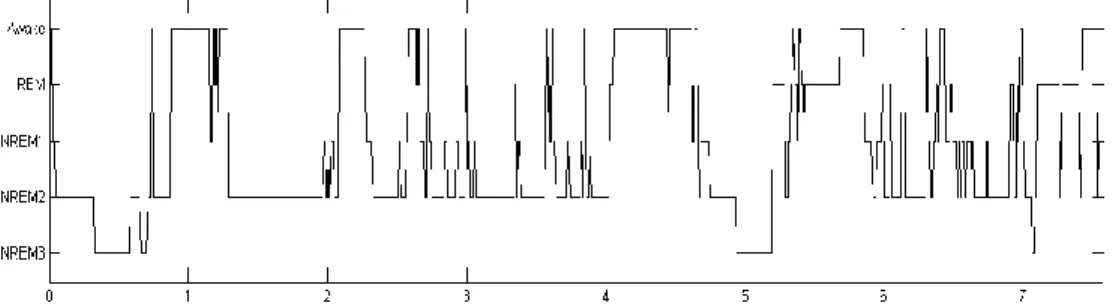
Polysomnography (PSG) consists in study of concurrent biophysiological electric signal shifts such as the electroencephalogram (EEG), electro-oculogram (EOG) and electromyogram (EMG) that occur during sleep. The PSG is commonly used as a diagnosis tool for the investigation of the sleep disorders and to characterize sleep fragmentation and sleep-disordered breathing such as sleep apnea (Obstructive Sleep Apnea / Hypopnea Syndrome, OSAHS). At the end of the sixties, Rechtschaffen and Kales [1] established a system of standardized rules and a scoring system for sleep stages of human subjects which enables the visual recognition by clinicians and technical experts of different sleep stages. Very recently, the American Academy of Sleep Medicine has updated these rules and technical specifications [2, 3] up to five: wakefulness, non-rapid eye-movement (NREM) sleep stages 1, 2 and 3, and rapid eye-eye-movement (REM) or paradoxical sleep (PS). Thus, the sleep stages are subsequently scored by sleep specialists every 30-second epoch. This graphic representation of the variations of the stages of sleep as a function of time leads to a temporal distribution called hypnogram (see Fig. 1.).
Because the PSG depicts the micro and macro-architecture of sleep, it has enabled to define many indicators called sleep characteristics used to assess sleep quality and so, to quantify sleep fragmentation. Then, from these characteristics and from their corresponding thresholds’ values, clinicians decide whether the patients’ sleep is fragmented or not. So, for mathematically modelling the sleep fragmentation diagnosis, a questionnaire has been sent to nine clinicians (three pulmonologists, three neurophysiologists and three technical experts) asking them to answer the following questions:
- What are the three main sleep characteristics enabling to diagnose a fragmented sleep? - What are the thresholds values for each of them?
- What is the importance (weight) of each of them in their diagnosis? It seems to be a consensus for the following three main sleep characteristics:
- the micro arousal rate (MAR),
- the number of sleep stages shifts (SSS) during the night recording,
- the number of intra sleep awakenings (ISA) by hour of total sleep time (hTST).
Concerning the thresholds values and the weights of these sleep characteristics from which the sleep can be considered as fragmented we observe some differences depending on each clinician’s specialization (pulmonologist, neurophysiologist and technical experts). So, the clinician’s diagnosis can be modelled according to three sleep characteristics (MAR, SSS, ISA) each having its own threshold and weight values.
In their seminal works, Lusted and Ledley [4, 5, 6] proposed many models from symbolic logic, probability, and value theory as a mathematical basis for logical analysis and in the use of machine aids to diagnosis. In the beginning of the eighties, Lezotte and Scheinok [7] discussed “The Role of Modelling Methods in Medical Diagnosis” using mathematical approaches which include cluster analysis, discriminant analysis, Bayesian methods, computer approaches, game theory, information theory, stochastic representations, stepwise procedures, decision analysis, and pattern recognition techniques. They pointed out some limitations of modelling methods in health care due to the complexity of the proposed model and also due to the sensitivity of the methodology to extract the informational content of the input parameters. Though mathematical models have been used in medical diagnosis since the sixties, it was only in the early nineties that they have been applied for analyzing the human sleep as exemplified by the article of Achermann and Borbély [8] who proposed a mathematical model for sleep regulation based on a continuous time dynamical systems. More particularly, it wasn’t until the last decades that several indicators of sleep quality were defined including the sleep fragmentation index (SFI) [9], the weighted-transition sleep fragmentation (WSFI) [10] and the sleep diversity index (SDI) [11]. Very recently, Swihart et al. [12] proposed a modelling of sleep fragmentation in sleep hypnograms based on the extension of current approaches of multivariate survival data analysis to clustered, recurrent event discrete-state discrete-time processes. Along with these mathematical approaches, the computational modelling of human sleep using Artificial Neural Networks for sleep stage scoring has been also developed since the nineties [13]. Thus, it appears that mathematical models of medical diagnosis and mathematical models of sleep fragmentation have been performed with the help of probabilistic methods, statistical methods, dynamical systems, artificial neural networks and sleep indicators. However, it does not seem, to our knowledge, that
there exists any mathematical model of sleep fragmentation diagnosis. Actually, the modelling of a clinician’s diagnosis is not an easy task if we take into account all the factors involved in such a process. Nevertheless, following the remark concerning the limitations of modelling methods highlighted by Lezotte and Scheinok [7], the aim of our work is to propose the most simple and consistent model of sleep fragmentation diagnosis. Our model, presented in Sec. 3, involving three sleep characteristics (MAR, SSS, ISA) each having its own threshold and weight values is thus based on the definition of a weighted arithmetic mean that we call below Mathematical
Diagnosis’ Index. Statistical methods are then used for these parameters’ estimation. Thresholds are deduced from Receiver Operating Characteristic (ROC) curves [14, 15] while weights are computed with the help of Principal Component Analysis (PCA) [16, 17], while. Hence, from a database of 111 PSG, a mathematical model of sleep fragmentation diagnosis is built for each clinician while taking into account its own specialization and which is a posteriori validated. 2. Material
2.1. Presentation of the PSG database
This retrospective and observational study (Protocol N° CH-2013-02) was conducted with the sleep laboratory of the Centre Hospitalier Intercommunal de Toulon la Seyne (CHITS). One hundred and eleven PSG under spontaneous breathing were selected in the sleep laboratory of the CHITS database: 55 from healthy adults and 56 from adult patients with a suspicion of obstructive sleep apnea syndrome (OSAS). The signals were recorded by a polysomnograph (Medatec®, Belgium). All the recordings were analyzed by nine clinicians (three pulmonologists, three neurophysiologists and three technical experts) and the sleep stages were encoded according to the American Academy of Sleep Medicine recommendations [2, 3].
2.2. Sleep characteristics extracted from the PSG recordings
Starting from our database, each polysomnographic (PSG) signal recording leads to the representation of the temporal distribution of sleep / wake stages with an hypnogram from which three sleep characteristics: Micro-Arousal Rate (MAR), Sleep Stages Shifts (SSS) and Intra Sleep Awakening (ISA) can be deduced among many others such as sleep latencies for example.
2.2.1. Micro Arousal Rate (MAR)
The micro-arousal rate (MAR) aka micro-arousal index, has been introduced by Guilleminault et al. [18] in 1988 and is defined by the total number of micro-awakenings divided by the total sleep time (TST) in hour. A micro-arousal is an abrupt shift in EEG frequency, which may include theta, alpha and / or frequencies greater than 16 Hz during 3 to 15 seconds. It is a change in the sleep micro-architecture that cannot be visualized on the hypnogram because it occurs during a sleep stage [19]. Thus, the micro-arousal rate has been introduced as the ‘gold standard’ to detect sleep fragmentation [19] and since it has been commonly considered as sleep characteristics reflecting sleep fragmentation.
2.2.2. Sleep Stages Shifts (SSS)
The number of sleep stages shifts (SSS) is defined as the number of transitions between the five sleep stages. According to Norman et al. [20] sleep fragmentation may be characterized with sleep stages shifts analysis.
2.2.3. Intra Sleep Awakenings (ISA)
An intra-sleep awakening is a stage encoded as an awake that occurs between the first and the last sleep stages. The total number of ISA and their duration are specified in the PSG report. Then, we can deduce the rate of intra-sleep awakenings (ISA) which is defined by the total number of intra sleep awakenings divided by the total sleep time (TST) in hour. According to Norman et al. [20], the number of intra sleep awakenings captures various potentially fragmenting behaviours which might impair continuity and has been shown to correlate with daytime sleepiness.
From a clinical point of view, sleep is considered as fragmented when there is a disorder of sleep continuity [20]. Subjectively, such a disorder can be revealed by intra-sleep awakenings unusually long or frequent. Objectively, on the PSG recordings, it can be also highlighted by the presence of many micro-arousals, frequent sleep stage changes, or abnormalities of the general architecture of the hypnogram. Moreover, detection of sleep fragmentation is of great importance because of its effect on the daytime function as pointed out by Stepanski et al. [21].
To diagnose sleep fragmentation, the clinician has to read the PSG recording, to encode the various sleep stages and to define the various events occurring on micro-architecture such as micro-arousals and the breathing events such as apneas and hypopneas [1, 2, 3]. At the end of the analysis, a PSG report is provided with all the sleep and breathing characteristics (some are presented in Tab. 1) and the hypnogram. For one polysomnography it takes about one hour for the clinician to read and to make a diagnosis. During the patient consultation, the clinician will decide whether the sleep is fragmented or not starting from the various data included in the PSG report such as the main sleep fragmentation characteristics (MAR, SSS, ISA) and the hypnogram. This will take about 3 minutes.
The choice of these three main sleep fragmentation characteristics is essentially based on an empirical knowledge of this sleep pathology which depends on the clinician specialization. The neurophysiologists focus on the sleep micro-architecture (micro-arousal rate) because their patients suffer from sleep disorders and neurological pathologies while the pulmonologists focus on breathing troubles and so, they will first analyse the macro-architecture, i.e., the hypnogram in which sleep stages shifts and intra-sleep awakenings can be visualized. This is generally when the diagnosis of sleep fragmentation cannot be clearly established that pulmonologists focus on micro-arousal rate as a second step.
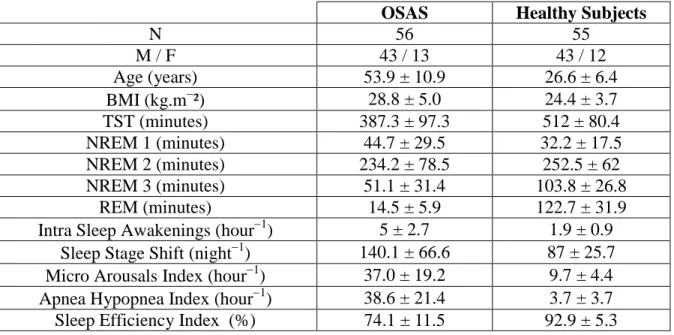
Clinical and sleep characteristics of the healthy subjects and the patients from our database of 111 PSG are presented in Tab. 1.
Table 1: Clinical and sleep characteristics of the normal subjects and the patients (i111). OSAS Healthy Subjects
N 56 55 M / F 43 / 13 43 / 12 Age (years) 53.9 ± 10.9 26.6 ± 6.4 BMI (kg.m²) 28.8 ± 5.0 24.4 ± 3.7 TST (minutes) 387.3 ± 97.3 512 ± 80.4 NREM 1 (minutes) 44.7 ± 29.5 32.2 ± 17.5 NREM 2 (minutes) 234.2 ± 78.5 252.5 ± 62 NREM 3 (minutes) 51.1 ± 31.4 103.8 ± 26.8 REM (minutes) 14.5 ± 5.9 122.7 ± 31.9
Intra Sleep Awakenings (hour1) 5 ± 2.7 1.9 ± 0.9 Sleep Stage Shift (night1) 140.1 ± 66.6 87 ± 25.7 Micro Arousals Index (hour1) 37.0 ± 19.2 9.7 ± 4.4 Apnea Hypopnea Index (hour1) 38.6 ± 21.4 3.7 ± 3.7 Sleep Efficiency Index (%) 74.1 ± 11.5 92.9 ± 5.3 2.2. Clinician’s thresholds values and weights of sleep characteristics
Concerning the thresholds values from which the sleep can be considered as fragmented, the result of our questionnaire for each group of clinicians is presented in Tab. 2.
Table 2: Sleep characteristics’ thresholds values from clinicians Thresholds Clin
MAR
(number/hTST) SSSClin (number/night) ISAClin (number/ hTST) Pulmonologists 15 10 10 100 100 110 1 3 3 Neurophysiologists 10 15 7 100 100 110 5 2 3 Technical experts 15 15 10 100 90 60 2 2 3
Concerning the importance, i.e. the weight of each sleep characteristic in the diagnosis of each clinician the result of our questionnaire is presented in Tab. 3.
Table 3: Sleep characteristics’ weights in each clinician’s diagnosis.
Weights Clin
MAR
w (%) wSSSClin (%) wISAClin (%) Pulmonologists 25 50 50 50 25 25 25 25 25 Neurophysiologists 50 25 70 25 15 20 25 60 10 Technical experts 40 10 10 50 10 30 10 60 60
Thus, the proposed mathematical model of sleep fragmentation diagnosis is mainly based on a set of three variables
X Y Z, ,
MAR SSS ISA, ,
each having two parameters:
X,wX
,
Y,wY
,
Z,wZ
which are respectively the thresholds and weights values for the MAR, the number of SSS and the rate of ISA. The comparison between the thresholds’ values provided by the clinicians themselves (Tab. 2) and those found in the literature highlights, of course, a quite good consistency. Indeed, by studying anonymous nocturnal polysomnograms from 10 normal subjects and 10 subjects with mild sleep disordered breathing, Norman et al. [21] found that the mean value of MAR for normal subjects is 14.8 5.1 , while for subjects with mild sleep disordered breathing they found 23.9 11.7 with a p-value ( p0.001). In the same work, Norman et al. [20] provide for normal subjects a mean value of the threshold for ISA equal to 3.00.9 with a p-value (p0.004). In a study on the effect of an antiepileptic on sleep including 10 healthy adults and 9 control subjects, Foldvary-Schaefer [22] found that during the baseline PSG the mean value of SSS for control subjects is 69.11 12.82 while during the follow-up PSG the mean value of SSS for control subjects is 78.78 20.78 with a p-value (p0.21).3. Method
3.1. Clinician’s diagnosis index
This population of 111 persons was diagnosed independently (double-blind procedure) by nine clinicians (three pulmonologists, three neurophysiologists and three technical experts). Each of them has established whether the sleep of each person (normal subject or adult patient) is fragmented or not. So, in order to transform their diagnosis into an index we use the following decision algorithm:
For each patient i, 1
i
D if the clinician considers patient’s sleep i as fragmented, 0
i
D if the clinician considers patient’s sleep i as not fragmented.
where D represents the result of each clinician’s diagnosis (fragmented or not fragmented) for i each patient i. From now on, we will call the clinician’s diagnosis represented by this index, CDI.
Remark. Let’s notice that the clinician’s diagnosis index (CDI) is not considered as a “gold
standard” but as the simple result of each clinician’s diagnosis which is based on his own experience and his own specialization (pulmonologist, neurophysiologist and technical expert).
3.2. Mathematic Diagnosis’ Index
Let
X Y Z, ,
MAR SSS ISA, ,
be the set of sleep characteristics andlet
xi x x1, 2,K,x111
be the specified finite list of values taken by the variable X, let
yi y y1, 2,K,y111
be the specified finite list of values taken by the variable Y, let
zi z z1, 2,K,z111
be the specified finite list of values taken by the variable Z,we define the thresholds vector as:
i X i Y i Z H x H y H z r (1)where H is the unit step function of Heaviside such that
1 if 0 if i A i A i A a H a a (2)and X, Y and Z are respectively the thresholds values of
X Y Z, ,
MAR SSS ISA, ,
.Then, we define the weights vector as
X X Y Z Y X Y Z Z X Y Z w w w w w w w w w w w w w r (3)
where w , X w and Y w are respectively the weights values of Z
X Y Z, ,
MAR SSS ISA, ,
. So, in order to define our Mathematic Diagnosis Index (MDI) we introduce the variable U that can take the specified finite list of values
ui u u1, 2,K,u111
. Then, the result of our mathematical diagnosis of sleep fragmentation is represented by
i i U d H u (4) where i T X
i X
Y
i Y
Z
i Z
X Y Z w H x w H y w H z u w w w w r r (5)where rT
H x
iX
,H yiY
,H ziZ
and U the threshold from which the sleep is considered as fragmented (see Sec. 3.3). From now on, we will call the mathematical diagnosis represented by this index, MDI.Remark. Thus, we have built a mathematical model of the sleep fragmentation diagnosis which
involves three variables
X Y Z , three thresholds , ,
X, Y, Z
and three weights
w w wX, Y, Z
. Obviously, the main difficulty lays in the determination of such thresholds and weights values with the best accuracy. A first approach had consisted in choosing the values provided by the clinicians themselves. Nevertheless, a great variability has been highlighted between the theoretical values they provided and the practical values that they use. So, in a second approach, we have chosen to compute statistically these values which are thus determined with a better accuracy. The same problem arises concerning the threshold value U of our MDI. Although, its theoretical value can be deduced mathematically (see Sec. 3.3. below), its practical value can be also computed statistically with a better accuracy.3.3. Threshold value determination of MDI
Let’s recall first that functions H involved in Eq. (5) are unit step function of Heaviside and so, they can only admit binary values equal to 0 or 1. Then, let’s suppose without loss of generality that wX wY wZ. The threshold U can be defined as:
X Y U X Y Z w w w w w (6)
The other cases can be easily deduced by circular permutations. As an example, we could consider that all these weights are identical and equal to 1. So, if we have wX wY wZ 1, the threshold is obviously U 2 3. However, as highlighted in Sec. 2.2, the weights given by each clinician to these sleep characteristics are not equal (see Tab. 2).
Remark. We will show also in the next section that the thresholds values of our MDI can be
statistically computed with a best accuracy. 3.4. Agreement between CDI and MDI
A measurement of the agreement between each clinician’s diagnosis (CDI) and each corresponding mathematical model (MDI) is then performed according to the Cohen's kappa coefficient [23] in order to test its efficiency in the sleep fragmentation diagnosis. So, Cohen's kappa coefficient MDI CDI is computed for the couple of variables
d D . i, i
The efficiency of our Mathematic Diagnosis’ Index (MDI) is then evaluated according to the amplitude of the Cohen's kappa coefficient CDI MDI for which Landis and Koch [24] provided a magnitude guideline for its interpretation (see Tab. 4).
Table 4: Magnitude guideline for interpretation of agreement of Cohen’s kappa coefficient [24] Kappa values 0 – 20% 21% – 40% 41% – 60% 61% – 80% 81% – 100% Interpretation slight fair moderate substantial almost perfect
3.5. Performance of our MDI
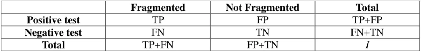
In order to assess the performance of our Mathematic Diagnosis’ Index (MDI) we also built the following confusion matrix (see Tab. 5).
Table 5: Confusion matrix for sleep fragmentation
Fragmented Not Fragmented Total
Positive test TP FP TP+FP
Negative test FN TN FN+TN
Total TP+FN FP+TN I
According to Bewick et al. [25] and Fawcett [26], in this confusion matrix also called contingency table, TP is the abbreviation for True Positive and represent the number of occurrence for which clinician’s diagnosis (CDI) and mathematic diagnosis’ index (MDI) have considered sleep as fragmented. While, TN (True Negative) is the number of times for which they have both considered sleep as not fragmented. These values located in the major diagonal represent the correct decisions made. On the contrary, if the sleep has been diagnosed as not fragmented by the clinicians and fragmented by our MDI, it is counted as a False Negative (FN). If the sleep has been diagnosed as fragmented by the clinicians and not fragmented by our MDI, it is counted as a False Positive (FP) and these numbers represent the errors – the confusion – between the various classes. Then, we compute the so-called sensitivity (Se) and specificity ratios (Sp) defined as follows (See also Altman et al. [27]). The sensitivity (Se) of a diagnostic test is the proportion of patients for whom the outcome is positive that are correctly identified by the test.
e TP S TP FN (7)
The specificity (Sp) is the proportion of patients for whom the outcome is negative that are correctly identified by the test.
Sp TN
TN FP
(8)
Then, sensitivity and specificity are combined to define the positive and negative likelihood ratios (LR+) and (LR). The positive likelihood ratio of a positive test result (LR+) is the ratio of the probability of a positive test result if the outcome is positive (true positive) to the probability of a positive test result if the outcome is negative (false positive). It is defined as
1 e p S LR S (9)
(LR+) represents the increase in odds favoring the outcome given a positive test result. Then, we can compute the pre-test probability (PRETP) of a positive outcome which is the prevalence of the outcome. The pre-test odds (PRETO) can be used to calculate the post-test probability (POSTO) of outcome with a Fagan’ nomogram [28] and can be expressed as follows:
-1
prevalence pre test odds
prevalence
(10) post test odds- pre test odds LR- (11) For a simpler interpretation, these post-test odds can be converted to a post-test probability (POSTP) using the expression:
-1
-post test odds post test probability
post test odds
(12)
Similarly, we can define the negative likelihood ratio (LR–) as the ratio of the probability of a negative test result if the outcome is positive to the probability of a negative test result if the outcome is negative. So, we have:
1 e p S LR S (13)
(LR–) represents the increase in odds favoring the outcome given a negative test result. We can also compute the pre-test probability of a negative outcome from which one can deduce the post-test probability defined by:
post test odds- pre test odds LR- (14) Similarly, these post-test odds can be converted to a post-test probability using expression (12). The performance of our Mathematic Diagnosis’ Index (MDI) will be then evaluated according to the positive and negative likelihood ratios (LR+) and (LR). According to Altman et al. [29] “a high (positive) likelihood ratio may show that the test is useful, but it does not necessarily follow that a positive test is a good indicator of the presence of the disease.” Deeks et al. [30] claim that a positive likelihood ratio LR above 10 and a negative likelihood LR below 0.1 are considered to provide strong evidence to rule in or rule out diagnoses respectively in most circumstances (see Tab. 6). This is transcribed by the increase between the pre-test and post-test probabilities which can be easily estimated while using the so-called Fagan’s nomogram [28].
Table 6: Magnitude guideline for interpretation of likelihood ratios
LR 1 2 – 5 5 – 10 > 10
Interpretation null Fair moderate substantial
LR > 0.5 0.2 – 0.5 0.1 – 0.2 < 0.1
3.6. Relevance of our MDI
In order to test the relevance of our Mathematic Diagnosis’ Index (MDI) in the diagnosis of sleep fragmentation we compare it to the so-called sleep fragmentation index (SFI) introduced by Haba-Rubio et al. [9] and defined by the addition of the number of sleep stage shift (Nsleep stage shift)
and the total number of awakenings (Nawakenings) divided by the total sleep time (TST) in hour:
SFI Nsleep stage shift Nawakenings TST
(15)
The computation of the Pearson’s correlation coefficient [31] between MDI and SFI will confirm the relevance of our Mathematic Diagnosis’ Index (MDI) for assessing the sleep fragmentation. 4. Results
From our database of 111 PSG recordings, we compute our Mathematic Diagnosis Index (MDI). Then, we measure the agreement between our MDI and each clinician’s diagnosis (CDI). However, as pointed out above, the main problem consists in the determination with a better accuracy the thresholds and weights values of the sleep characteristics as well as the threshold value of our MDI. So, in the next section 4.1 & 4.2, we propose to compute them statistically.
4.1 Thresholds values determination
X, Y, Z
As recalled above, although these thresholds values have been provided by each clinician (see Tab. 2) the fragmentation thresholds value
X, Y, Z
of each sleep characteristic
X Y Z, ,
MAR SSS ISA, ,
can be statistically computed while using the so-called Receiver Operating Characteristic (ROC) curves [14]. Starting from our database of 111 PSG each threshold is given by the maximum value of the Youden’s index. By considering the clinician’s diagnosis D as the reference we plotted for each couple i
x D , i, i
y D and i, i
z D the i, i
fraction of true positives out of the total actual positives (sensitivity) vs. the fraction of false positives out of the total actual negatives (1 specificity), at various threshold settings. Thus, the maximum value of the Youden’s index has enabled to find the appropriate threshold for each sleep characteristic. We called clinX , clin
Y
and clin Z
the thresholds given by the clinicians (see Tab. 2) and XROC, YROC and ZROC the thresholds determined with ROC curves (see Tab. 7). Then, the performance of our diagnostic variable has been quantified by calculating the area under the ROC curve (AUROC) [15]. By building ROC curves for each sleep characteristic
X Y Z, ,
MAR SSS ISA, ,
for each clinician (three pulmonologists, three neurophysiologists and three technical experts) we determine the fragmentation thresholds values (see Tab. 7).Table 7: Sleep characteristics’ thresholds values from ROC curves with p0.01 Threshold MARROC (number/hTST)
ROC SSS (number/night) ROC ISA (number/hTST) Pulmonologists 20 12 12 99 90 104 2.24 2.55 2.73 AUROC1 82% 78.1% 92.8% 90.6% 91.7% 77.4% 87% 83.6% 78.4% Neurophysiologists 11.7 20 18.3 110 95 109 2.51 2.49 2.73 AUROC 95.4% 79% 90.2% 73.1% 91.7% 87.7% 80.5% 94.5% 89.4% Technical experts 12 20 18.3 110 92 92 2.51 2.14 2.49 AUROC 90% 77.2% 76.9% 81.5% 83.9% 89.9% 81.1% 87.2% 89.6%
A comparison between the sleep characteristics’ thresholds for sleep fragmentation given by the clinicians themselves (Tab. 2) and those given by ROC curves (Tab. 7) highlights a great variability between the theoretical values they provided (Tab. 2) and the practical values that they use (Tab. 7).
4.2 Weights values determination
w w wX, Y, Z
As recalled above, although these weights values have been provided by each clinician (see Tab. 3) the fragmentation thresholds value
w w wX, Y, Z
of each sleep characteristic
X Y Z, ,
MAR SSS ISA, ,
can be statistically computed while using the so-called Principal Component Analysis [16, 17]. Starting from our database of 111 PSG each weight is given by the Pearson’s correlation [31] between each sleep characteristic and each corresponding clinician’s diagnosis, i.e.,
x D , i, i
y D and i, i
z D . Thus, we obtain for each couple a correlation i, i
coefficient, respectively , and . Then, we normalize these values and we obtain:
wPCAX ,wYPCA,wZPCA
, ,
We called wXclin, wYclin and wclinZ the weights values given by the clinicians (see Tab. 3) and wPCAX ,
PCA Y
w and wZPCA the weights values determined with PCA curves (see Tab. 8).
Table 8: Sleep characteristics’ weights values from PCA with p0.01 Weight wMARPCA (%)
PCA SSS w (%) wISAPCA (%) Pulmonologists 29.4 25 39.5 35.85 39.6 28.35 34.75 35.4 32.15 Neurophysiologists 40.3 25.75 33.75 27.2 36.25 32 32.5 38 34.25 Technical experts 35.64 27.15 25.77 31.7 34.58 36.8 32.66 38.27 37.43 1
Area Under ROC curve is equal to the probability that a classifier will rank a randomly chosen positive instance higher than a randomly chosen negative one (assuming “positive” ranks higher than “negative”) [15].
A comparison between the values of the sleep characteristics’ weights for sleep fragmentation given by the clinicians themselves (Tab. 3) and those given by PCA (Tab. 8) also highlights a great variability between the theoretical values they provided (Tab. 3) and the practical values that they use (Tab. 8).
4.3. Agreement between CDI and MDI
In Sec. 3.3., it has been stated that the thresholds values of our MDI can be mathematically deduced from Eq. (6). However, it can also be statistically computed with a better accuracy while using the so-called Receiver Operating Characteristic (ROC) curves [14]. Starting from our database of 111 PSG each threshold is given by the maximum value of the Youden’s index. By considering the clinician’s diagnosis D as the reference we plotted for each couple i
d D the i, i
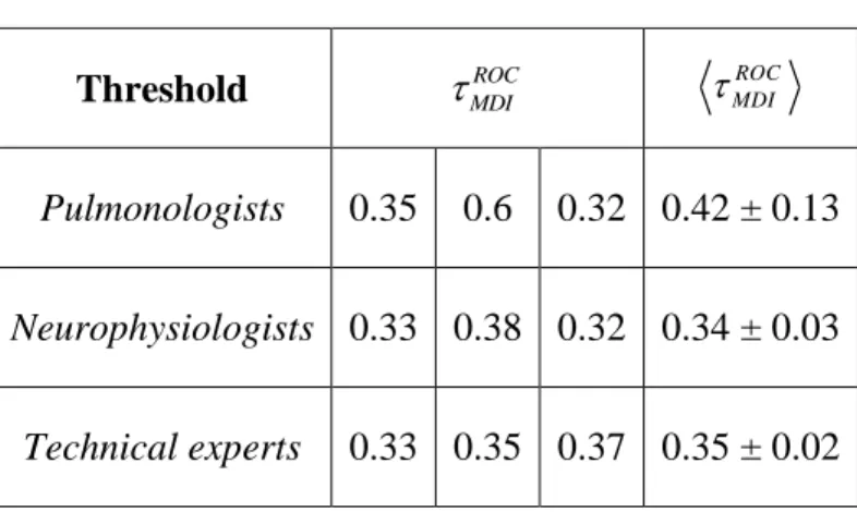
fraction of true positives out of the total actual positives (sensitivity) vs. the fraction of false positives out of the total actual negatives (1 specificity), at various threshold settings. Thus, the maximum value of the Youden’s index has enabled to find the appropriate threshold value of our MDI for each clinician. We called MDIROCthe thresholds of our MDI determined with ROC curves (see Tab. 9). Then, the performance of our diagnostic variable has been quantified by calculating the area under the ROC curve (AUROC) [15].
Table 9: Thresholds values of MDI withp0.01 Threshold MDIROC
ROC MDI Pulmonologists 0.35 0.6 0.32 0.42 ± 0.13 Neurophysiologists 0.33 0.38 0.32 0.34 ± 0.03 Technical experts 0.33 0.35 0.37 0.35 ± 0.02
Then, we compute the agreement between MDI and CDI with fragmentation thresholds and weights values obtained statistically (Tab. 7 & 8) and while using the thresholds values of MDI also determined statistically (see Tab. 10).
Table 10: Cohen’s kappa coefficient between MDI and CDI Clinicians CDI MDI
(%) CDI MDI (%) Pulmonologists 76.09 70.86 72.05 73.00 ± 2.24 Neurophysiologists 74.60 88.99 61.51 74.70 ± 11.62
So, according to Landis et al. [24] (see Tab. 4), the agreement between each clinician’s diagnosis (CDI) and each corresponding mathematical model (MDI) goes from substantial ( 61%) to
almost perfect ( 81%), according to their specialization. Moreover, the mean value of the agreements of each group is also substantial ( 73%). Then, to test the performance of our MDI we built the confusion matrix (Tab. 5) for the three groups of clinicians (pulmonologists,
neurophysiologists and technical experts). The results are presented in Tab. 11.
Table 11: Confusion matrices for sleep fragmentation for the three groups of clinicians
Pulmonologists 57 7 6 41 55 6 10 40 66 8 6 31 Neurophysiologists 65 5 8 33 60 3 3 45 62 9 11 29 Technical experts 66 3 7 35 67 5 11 28 59 5 10 37
From these matrices we deduce the main statistical characteristics for each clinician and so for each group of clinicians. The results are presented in Tab. 12.
Table 12: Statistical characteristics for the three group of clinicians (pulmonologists, neurophysiologists, technical experts)
Clinicians Pulmonologists Neurophysiologists Technical experts PPV2 (%) 89.06 90.16 89.18 92.85 95.23 87.32 95.65 93.05 92.18 NPV3 (%) 87.23 80 83.78 80.48 93.75 72.5 83.33 71.79 78.72 e S 57 63 55 65 66 72 65 73 60 63 62 73 66 73 67 78 59 69 p S 41 48 40 46 31 39 33 38 45 48 29 38 35 38 28 33 37 42 LR 6.2 6.48 4.46 6.76 15.23 3.58 11.45 5.66 7.18 LR 0.11 0.17 0.10 0.12 0.05 0.19 0.10 0.16 0.16 PRETP (%) 56.75 58.55 64.86 65.76 56.75 65.76 65.76 70.27 62.16 PRETO 1.3125 1.4130 1.8461 1.9210 1.3125 1.9210 1.9210 2.36 1.6428 POSTO 8.1428 9.1667 8.25 13 20 6.88 22 13.4 11.8 POSTP(%) 89.06 90.16 89.18 92.85 95.23 87.32 95.65 93.05 92.18 P (%) 32.30 31.60 24.32 27.09 38.48 21.55 29.88 22.78 30.02 2
Positive Predictive Value. 3 Negative Predictive Value.
Concerning the pulmonologists’ group we found (see Tab. 12) the following positive likelihood ratios LR 4.46, LR 6.2 and LR 6.48. This means that a person (chosen among our database of 111 PSG recordings) with a fragmented sleep is about 4.46 (respectively 6.2 and 6.48) times more likely to have a positive test than a person whose sleep is not fragmented. We also found the following negative likelihood ratios LR 0.10 1 10 ,
0.11 1 9
LR and LR 0.17 1 6 . This means that the probability of having a negative test for individuals with sleep fragmented is 0.1 (respectively 0.11, 0.17) times of that of those with sleep not fragmented. In other words, individuals with sleep not fragmented are about ten (respectively 9, 6) times more likely to have a negative test than individuals with sleep fragmented. Moreover, the difference (P) between pre-test and post-test probabilities, which corresponds to a gain in diagnostic, ranges from 24.32% to 32.30%.
For the neurophysiologists’ group, the following positive likelihood ratios LR 3.58, 6.76
LR and LR 15.23 and the following negative likelihood ratios LR 0.05 1 20 , 0.12 1 8
LR and LR0.19 1 5 have been obtained (see Tab. 12). For this group, the difference between pre-test and post-test probabilities, which corresponds to a gain in diagnostic, ranges from 21.55% to 38.48%.
As regards the technical experts’ group we obtained (see Tab. 12) the following positive likelihood ratios LR 5.66, LR 7.18 and LR 11.45. and the following negative likelihood ratios LR 0.10 1 10 , LR0.16 1 6 and LR 0.16 1 6 . For this group, the difference between pre-test and post-test probabilities, which corresponds to a gain in diagnostic, ranges from 22.78% to 30.02%.
Moreover, the agreement between two clinician’s diagnosis (CDI-CDI) of the same specialization, i.e., belonging to the same group (pulmonologists, neurophysiologists, technical
experts) and of different specializations has been also computed (see Tab. 13).
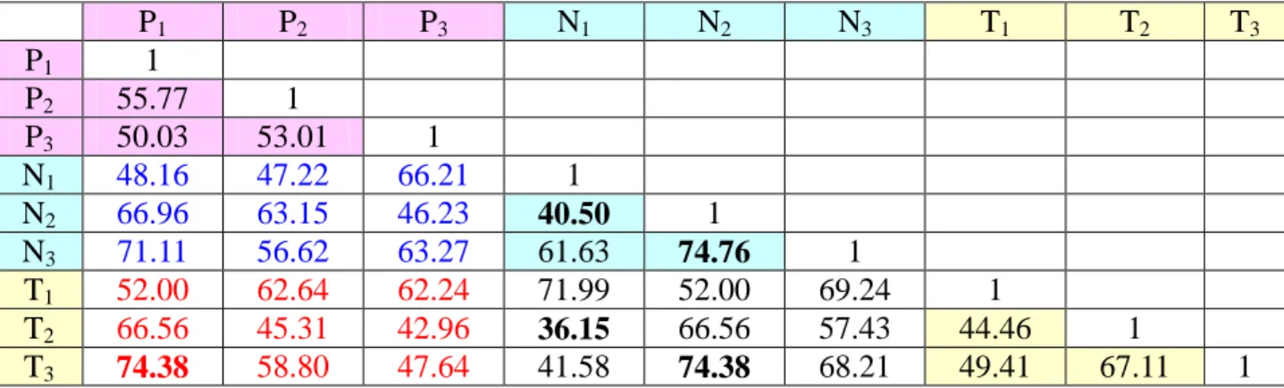
Table 13: Cohen’s kappa coefficient CDI CDI (%) between two clinician’s diagnosis (CDI-CDI)
P1 P2 P3 N1 N2 N3 T1 T2 T3 P1 1 P2 55.77 1 P3 50.03 53.01 1 N1 48.16 47.22 66.21 1 N2 66.96 63.15 46.23 40.50 1 N3 71.11 56.62 63.27 61.63 74.76 1 T1 52.00 62.64 62.24 71.99 52.00 69.24 1 T2 66.56 45.31 42.96 36.15 66.56 57.43 44.46 1 T3 74.38 58.80 47.64 41.58 74.38 68.21 49.41 67.11 1
According to Landis et al. [24] (see Tab. 4), we observe from Tab. 13 that the agreement between two clinicians’ diagnosis (CDI-CDI) of the same specialization (same group) ranges from
moderate (CDI CDI 40.50%) to substantial (CDI CDI 74.76%). We also observe that the
agreement between two clinicians’ diagnosis (CDI-CDI) of different specializations ranges from fair (CDI CDI 36.15%) to substantial (CDI CDI 74.38%).
Then, the agreement between two mathematical models of clinician’s diagnosis (MDI-MDI) of the same specialization, i.e., belonging to the same group (pulmonologists, neurophysiologists,
technical experts) and of different specializations has been also computed (see Tab. 14).
Table 14: Cohen’s kappa coefficient MDI MDI (%) between two mathematical models of clinician’s diagnosis (MDI-MDI)
P1 P2 P3 N1 N2 N3 T1 T2 T3 P1 1 P2 69.00 1 P3 47.70 74.26 1 N1 47.75 69.53 84.47 1 N2 68.73 85.45 65.68 53.77 1 N3 64.80 75.36 82.27 70.86 74.63 1 T1 46.69 71.24 86.69 98.09 55.64 72.99 1 T2 70.61 77.50 60.05 49.25 84.32 70.54 51.53 1 T3 66.79 87.32 67.04 55.31 98.18 76.19 57.21 85.88 1
Still according to Landis et al. [24] (see Tab. 4), we observe from Tab. 14 that the agreement between two mathematical models of clinicians’ diagnosis (MDI-MDI) of the same specialization (same group) ranges from moderate (MDI MDI 47.70%
) to almost perfect (MDI MDI 85.88% ). We also found that the agreement between two mathematical models of clinicians’ diagnosis (MDI-MDI) of different specializations ranges from moderate (MDI MDI 47.75%) to almost
perfect (MDI MDI 98.09%).
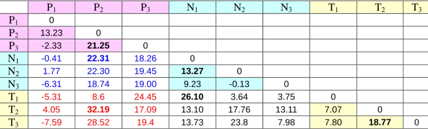
Table 15: Difference between Cohen’s kappa coefficient MDI MDI CDI CDI (%)
P1 P2 P3 N1 N2 N3 T1 T2 T3 P1 0 P2 13.23 0 P3 -2.33 21.25 0 N1 -0.41 22.31 18.26 0 N2 1.77 22.30 19.45 13.27 0 N3 -6.31 18.74 19.00 9.23 -0.13 0 T1 -5.31 8.6 24.45 26.10 3.64 3.75 0 T2 4.05 32.19 17.09 13.10 17.76 13.11 7.07 0 T3 -7.59 28.52 19.4 13.73 23.8 7.98 7.80 18.77 0
Table 15 enables to quantify the difference between the agreement between two mathematical
models of clinician’s diagnosis (MDI-MDI) and the agreement between two clinicians’ diagnosis (CDI-CDI). We observe that the agreement is improved up to 21.25% for pulmonologists, up to 13.27% for neurophysiologists and up to 18.77% for technical experts. Moreover, we also notice that the agreement between the groups of pulmonologists and of neurophysiologists (in blue) is improved up to 22.31%. While the agreement between the groups of pulmonologists and of
technical experts (in red) is improved up to 32.19% and the agreement between the groups of neurophysiologists and of technical experts (in black) is improved up to 26.10%
Finally, from our database of 111 PSG recordings, we compute the Pearson’s correlation coefficient between the mathematical model (MDI) of each clinician’s diagnosis (pulmonologist, neurophysiologist and technical expert) and the sleep fragmentation index (SFI). The results are presented in Table 16.
Table 16: Pearson’s correlation coefficient r between MDI and SFI withp0.01 Clinicians MDI SFI
r (%) rCDI SFI (%) Pulmonologists 74.15 71.79 75.02 73.65 ± 1.36 Neurophysiologists 74.34 74.27 78.25 75.62 ± 1.86 Technical experts 75.80 71.85 73.33 73.66 ± 1.63
From these results, it appears that each mathematical model (MDI) of the nine clinicians (pulmonologists, neurophysiologists, technical experts) belonging to the three groups is strongly correlated with the sleep fragmentation index (SFI) (r71% with p0.01). It follows that we can consider that our MDI is relevant for assessing the sleep fragmentation.
5. Discussion
By considering, as several authors [9, 19, 20], that sleep fragmentation diagnosis is essentially based on three main sleep characteristics which are the micro arousal rate (MAR), the number of sleep stages shifts (SSS) and the rate of intra sleep awakenings (ISA) each having its own fragmentation threshold value and each being more or less important (weight) in the clinician’s diagnostic according to his specialization (pulmonologist, neurophysiologist and technical expert), we have built a mathematical model of sleep fragmentation diagnosis for each clinician we called Mathematic Diagnosis’ Index (MDI) involving thresholds and weights values.
From a database of 111 PSG, consisting of 55 healthy adults and 56 adult patients with a suspicion of obstructive sleep apnoea syndrome (OSAS), a sleep fragmentation diagnosis has been performed independently by nine clinicians (three pulmonologists, three neurophysiologists and three technical experts) in a double blind procedure and by our mathematical model for each clinician. This has enabled to compute statistically the thresholds and weights values with a better accuracy. Then, a statistical analysis based on the use of the so-called Cohen’s kappa coefficient [23] has shown (Tab. 10) that the agreement between each of the nine clinician’s diagnosis (CDI) and each corresponding mathematical model (MDI) goes from substantial ( 61%) to almost
perfect ( 81%), according to their specialization.
Moreover, the use of our mathematical model of sleep fragmentation diagnosis MDI has provided for all nine clinicians a positive likelihood ratio LR ranging from 3.58 to 11.45 and a negative likelihood ratio LR ranging from 0.05 to 0.19. So, according Altman et al. [29] and Deeks et al. [30], this indicates that the test result (MDI) has an effect on increasing the probability of fragmented sleep presence which ranges from moderate to substantial.
Obviously, these statistical computations are dependent on the number of clinicians which may induce a great variability in the CDI measurements. As pointed out by Pr. Collop [32] “a significant variability exists between polysomnography technologists in the scoring of sleep
studies particularly regarding respiratory events.” Of course such variability has been observed between two clinicians of the same specialization and also between two clinicians of different specializations (Tab. 13). We observed that the agreement between two clinicians’ diagnosis (CDI-CDI) of the same specialization ranges from moderate (CDI CDI 40.50%) to substantial (CDI CDI 74.76%) while it ranges from fair (CDI CDI 36.15%) to substantial (CDI CDI 74.38%) for clinicians’ diagnosis (CDI-CDI) of different specializations.
However, let’s recall on the one hand that each clinician’s diagnosis index (CDI) has not been treated as a “gold standard” and on the other hand that our Mathematic Diagnosis’ Index (MDI) has not been built as a “universal model” of the sleep fragmentation diagnosis. On the contrary, it is important to point out that there is a biunivocal correspondence between each CDI and each MDI. In other words, it means that we have built a specific MDI for each clinician depending on his specialization. Nevertheless, despite this variability, we found that the agreement between each of the nine clinician’s diagnosis (CDI) and each corresponding mathematical model (MDI) goes from substantial to almost perfect as highlighted in Tab. 10.
Moreover, we observed from Tab. 15 that the difference between the agreement between two
mathematical models of clinician’s diagnosis (MDI-MDI) and the agreement between two clinicians’ diagnosis (CDI-CDI) is improved for clinicians of same specialization and also for clinicians of different specializations. Thus, we can consider that our MDI reduces the variability between “polysomnography technologists”, i.e., between the three groups of pulmonologists, neurophysiologists and technical experts.
Finally, from Tab. 16 we have found a strong correlation (r71% with p0.01) between our MDI and the SFI for all the nine clinicians whether they belong to the same group or to a different group. As a consequence, our MDI is relevant for assessing sleep fragmentation.
So, it follows from these results that the proposed mathematical model of sleep fragmentation diagnosis of each clinician we called Mathematic Diagnosis’ Index (MDI) based on the three main sleep characteristics (MAR, SSS, ISA) each having its own threshold and weight values for each clinician is a posteriori. According to Lezotte and Scheinok [7] the determination of these thresholds and weights values (input parameters) could have been a severe obstacle in any modelling attempt as evidenced by the differences observed between the theoretical values given by each clinician (see Tab. 2 & 3) and the practical values deduced from statistical computations (see Tab. 7 & 8). These differences represent what we could call a “problem of self interpretation” which leads to a distortion between the values that the clinician thinks he has used and the values he has really used in his own diagnosis. Nevertheless, it has been shown in this work that the thresholds values can be statistically deduced from ROC curves while the weights values can be statistically computed from PCA. Thus, it appears that these thresholds and weights values should be considered as the “signature” of each clinician’s diagnosis. So, as a perspective of research, we propose to validate each mathematical model (MDI) built for each clinician, while testing them on another database of 405 PSG resulting from a prospective multicenter protocol (Protocol N° CH-2014-02) and involving the same clinicians with their own thresholds and weights values that have been statistically computed in this work. If, as we expect, the agreement between each mathematical model (MDI) and each corresponding clinicians’ diagnosis (CDI) is substantial or almost perfect, then, our MDI will be validated a priori. Some preliminary results have enabled to confirm that these mathematical model (MDI) would be validated a priori. Indeed, from a CHITS database of 32 PSG recordings diagnosed by two clinicians (a pulmonologist and a neurophysiologist) we have found that the agreement between
each clinician’s diagnosis (CDI) and each corresponding mathematical model (MDI) is almost
perfect ( 81%) for both clinicians.
The heterogeneity of the demographic data presented in Table 1, i.e., the significant age difference between the two groups included in the study as well as the BMI difference, is another aspect that should have been also considered. Thus, such differences may have influenced the results to an extent that they would have simply reflected the existence of a spontaneous evolution in sleep quality with age rather than a real difference between normal and pathologic. Moreover, the diagnosis potential of the explored feature as valid indexes of pathologically fragmented sleep may have been discussed. Of course, such an heterogeneity should have been taken into account into our mathematical model (MDI) of the sleep fragmentation diagnosis. However, in this work, our aim was to show that it is possible to build a simple and consistent mathematical model of sleep fragmentation diagnosis of clinicians according to their specialization (pulmonologist, neurophysiologist and technical expert). Although in this modelling we have made some strong assumptions and certain choices about the selected sleep characteristics (we could have chosen some others), it appears from the substantial agreement between each MDI and each CDI highlighted in Tab. 10 that our mathematical model is a
posteriori validated. Let’s notice that if many mathematical models in medical diagnosis have
been developed for a long time (see for example [4-13]), it doesn’t seem, to our knowledge, that there exists any mathematical model of sleep fragmentation diagnosis.
6. Conclusion
In this work, we have built a simple and consistent mathematical model of sleep fragmentation diagnosis we called Mathematic Diagnosis’ Index (MDI) based on three main sleep characteristics (MAR, SSS, ISA) each having its own threshold and weight values for each clinician according to his specialization. Then, from a database of 111 PSG, consisting of 55 healthy adults and 56 adult patients with a suspicion of obstructive sleep apnoea syndrome (OSAS), a sleep fragmentation diagnosis has been performed independently by nine clinicians (three pulmonologists, three neurophysiologists and three technical experts) in a double blind procedure and by our mathematical model for each clinician. A statistical analysis has shown that the agreement between each of the nine clinician’s diagnosis (CDI) and each corresponding mathematical model (MDI) goes from substantial ( 61%) to almost perfect ( 81%), according to their specialization. Moreover, the computation of likelihood ratios deduced from the confusion matrices has exhibited a gain in diagnostic which ranges from 21% to 30% for each group of clinicians (pulmonologists, neurophysiologists, technical experts). Finally, the computation of the Pearson’s correlation coefficient between our MDI and the SFI has highlighted a strong correlation (r71%) which confirms that our MDI is relevant for assessing the sleep fragmentation. So, it follows from these results that our mathematical model MDI is a
posteriori validated for each clinician and could be very useful as a diagnostic aid.
Acknowledgements
Authors would like to thank the technical experts of CHITS for their important contribution to this work as well as the referees for their very helpful advices which have contributed to greatly improve the presentation and the content of this work, all the staff of the sleep laboratory of CHITS including Dr. Isabelle SUFFIA, PhD, Study Site Coordinator. The applet created in MatLab (MDI.m) for computing our MDI is available by simple request to the authors.
References
[1] A. Rechtschaffen, A. Kales, A manual of standardized terminology, techniques, and scoring system for sleep stages of human subjects, U.S. Government Printing Service, Washington D.C. Public Health Service, 1968.
[2] C. Iber, S. Ancoli-Israel, A. Chesson, S.F. Quan, The AASM Manual for the Scoring of Sleep and Associated Events: Rules, Terminology and Technical Specifications, 1st ed.: Westchester, Illinois: American Academy of Sleep Medicine, 2007.
[3] R. Berry et al., The AASM Manual for the scoring of Sleep and Associated Events: Rules Terminology and Technical Specifications, Version 2.0. Darien, IL: American Academy of Sleep Medicine, 2012.
[4] L.B. Lusted and R.S. Ledley, Mathematical Models in Medical Diagnosis, Journal of Medical Education 35 (3) (March 1960) 214–222.
[5] R.S. Ledley and L.B. Lusted, Reasoning foundations of medical diagnosis; symbolic logic, probability, and value theory aid our understanding of how physicians reason, Science 130 (3366) (July 3, 1959) 9–21.
[6] R.S. Ledley and L.B. Lusted, The Use of Electronic Computers in Medical Diagnosis. Proc. I.R.E. 47 (Medical Electronic Issue, Nov. 1959) 1970–1977.
[7] D. Lezotte and P.A. Scheinok, The role of modeling methods in medical diagnosis, Journal of Medical System 5 (3) (1981) 197–209.
[8] P. Achermann, D. J. Dijk, D. P. Brunner and A. A. Borbély, A model of human sleep homeostasis based on EEG slow-wave activity: quantitative comparison of data and simulations. Brain Research Bulletin 31 (1993) 97–113.
[9] J. Haba-Rubio, V. Ibanez, E. Sforza, An alternative measure of sleep fragmentation in clinical practice: the sleep fragmentation index, Sleep Medicine 5 (2004) 577–581.
[10] V. Swarnkar, U.R. Abeyratne, C. Hukins, B. Duce, A state transition-based method for quantifying EEG sleep fragmentation, Medical and Biological Engineering and Computing 47 (10) (2009) 1053–1061.
[11] R. Naeck, D. D'Amore, M.-F. Mateo, A. Elias, J.-Ph. Suppini, A. Rabat, Ph. Arlotto, M. Grimaldi, E. Moreau and J.-M. Ginoux, Sleep Diversity Index for sleep fragmentation analysis, Journal of Nonlinear Systems and Applications (in press).
[12] B.J. Swihart, N.M. Punjabi, C.M. Crainiceanu, Modeling sleep fragmentation in sleep hypnograms: An instance of fast, scalable discrete-state, discrete-time analyses, Computational Statistics & Data Analysis 89 (September 2015) 1–11.
[13] N. Schaltenbrand, R. Lengelle, M. Toussain, R. Luthringer, G. Carelli, A. Jacqmin, E. Lainey, A. Muzet, J.-P. Macher, Sleep stage scoring using the neural network model: comparison between visual and automatic analysis in normal subjects and patients, Sleep 19 (1) (Jan 1996) 26–35.
[14] J.P. Egan, Signal Detection Theory and ROC Analysis, Series in Cognition and Perception. Academic Press, New York, 1975.
[15] J.A. Hanley, B.J. McNeil, The Meaning and Use of the Area under a Receiver Operating Characteristic (ROC) Curve, Radiology 143 (1) (1982) 29–36.
[16] H. Hotelling, Analysis of a Complex of Statistical Variables into Principal Components, Journal of Educational Psychology, 24 (6 & 7) (1933) 417–441 & 498–520.
[17] I.T. Jolliffe, Principal Component Analysis, Second edition Springer Series in Statistics, New York: Springer-Verlag New York, 2002.
[18] C. Guilleminault, M. Partinen, Ma. Quera-Salva, B. Hayes, W.C. Dement, G. Nino-Murcia, Determinants of daytime sleepiness in obstructive sleep apnea, Chest 94 (1988) 32–37.
[19] M. Bonnet et al. EEG arousals: scoring rules and examples: a preliminary report from the Sleep Disorders Atlas Task Force of the American Sleep Disorders Association, Sleep 15 (2) (1992) 173–184.
[20] R.G. Norman, M.A. Scott, I. Ayappa, J.A. Walsleben, D.M. Rapoport, Sleep continuity measured by survival curve analysis, Sleep 29 (12) (2006) 1625–1631.
[21] E.J. Stepanski, The effect of sleep fragmentation on daytime function, Sleep 25 (3) (2002) 268–276.
[22] N. Foldvary-Schaefer, I. De Leon Sanchez, M. Karafa, D. Dinner, H.H. Morris, Gabapentin Increases Slow-wave Sleep in Normal Adults, Epilepsia 43 (12) (2002) 1493–497.
[23] J. Cohen, A coefficient of agreement for nominal scales, Educational and Psychological Measurement 20 (1) (1960) 37–46.
[24] J.R. Landis and G.G. Koch, The measurement of observer agreement for categorical data, Biometrics 33 (1) (1977) 159–174.
[25] V. Bewick, L. Cheek, J. Ball, Statistics Review 13: Receiver Operating Characteristics Curves, Critical Care 8 (6) (2004) 508–512.
[26] T. Fawcett, ROC graphs: Notes and practical considerations for researchers, ReCALL 31 (HPL-2003-4) (2004) 1–38.
[27] D.G. Altman and J.M. Bland, Diagnostic tests 1: sensitivity and specificity, BMJ 11 (1994 Jun) 308 (6943) 1552.
[28] T.J. Fagan, Nomogram for Bayes's theorem, New England Journal of Medicine 293 (5) (1975) 257.
[29] D.G. Altman, J.M. Bland, Diagnostic tests 2: predictive values, BMJ 9 (1994 Jul) 309 (6947) 102.
[30] J.J. Deeks, D.G. Altman, Diagnostic tests 4: likelihood ratios, BMJ 329 (2004 Jul) 168–169. [31] K. Pearson, Studies in the history of Statistics and probability, Biometrika, 13 (1920) 25–45. [32] N.A. Collop, Scoring variability between polysomnography technologists in different sleep laboratories, Sleep Medicine 3 (2002) 43–47.
![Table 4: Magnitude guideline for interpretation of agreement of Cohen’s kappa coefficient [24]](https://thumb-eu.123doks.com/thumbv2/123doknet/14620548.733699/10.918.127.791.994.1059/table-magnitude-guideline-interpretation-agreement-cohen-kappa-coefficient.webp)