Dans le cadre d’une cotutelle avec l’Université de São Paulo (USP)
Extraction photométrique en vol des étoiles de la mission PLATO:
Masques optimaux pour la détection de planètes extra-solaires
In-flight photometry extraction of PLATO targets:
Optimal apertures for detecting extra-solar planets
Soutenue par
Victor Atilio MARCHIORI
Le 16 September 2019 École doctorale no127 Astronomie et Astrophysique d’Île-de-France (AAIF) Spécialité Astronomie et Astrophysique Composition du jury : Marie-Christine ANGONIN
Professeur, Observatoire de Paris Présidente
Magali DELEUIL
Professeur, Université Aix Marseille Rapporteure
Suzanne AIGRAIN
Professeur, University of Oxford Rapporteure
Eduardo JANOT PACHECO
Professeur, Universidade de São Paulo Examinateur
Frédéric BAUDIN
Astronome, Université Paris-Sud Examinateur
Alexandre SANTERNE
Astronome adjoint, Univ. Aix Marseille Examinateur
Réza SAMADI
Astronome, Observatoire de Paris Directeur de thèse
Fábio de Oliveira FIALHO
In-flight photometry extraction of PLATO targets:
Optimal apertures for detecting extra-solar planets
Thesis presented to the Polytechnic School of the University of São Paulo for obtaining the degree of Doctor of Engineering. Thesis presented to the Paris Observatory for ob-taining the degree of PhD in Astronomy and Astrophysics.
Universidade de São Paulo / Observatoire de Paris
Departamento de Telecomunicações e Controle da Escola Politécnica (PTC/EPUSP) / Laboratoire d’Etudes Spatiales et d’Instrumentation en Astrophysique (LESIA)
Engenharia de Sistemas / Astronomie et Astrophysique
Supervisor: Fábio de Oliveira Fialho (EPUSP)
Supervisor: Réza Samadi (LESIA)
Meudon
2019
To my mom, Margarete, and my dad, Atilio. To my grandma, Maria.
To my friends.
I am deeply grateful to Marie-Christine, Suzanne, Magali, Eduardo, Frédéric, and Alexandre for having accepted being members of my thesis jury and for having dedicated their valuable time reading this manuscript. I give special thanks to the reviewers, Suzanne and Magali, for having also devoted their time to write the thesis report.
I would like to thank the French National Centre for Space Studies (CNES), the Paris Observatory – PSL and the Brazilian National Council for Scientific and Technological Development (CNPq) for having provided me financial support to develop this thesis.
I acknowledge the directorate and the members of the Doctoral School of Astronomy and Astrophysics of Ile-de-France (ED127) for their readiness to support PhD students whenever needed. I express my gratitude to the administration of LESIA and to the members of Pôle Étoile for their kindness and for having provided me excellent working conditions throughout my whole PhD. In especial, I thank Benoît, Bram, Caroline, Charlotte, Charly, Coralie, Daniel, Eric, Jordan, Marie-Jo, Morgan, Kévin, Rhita, Richard, Steven and Yveline for the great moments we shared together in the everyday working life au Labo.
I would like to express the deepest appreciation to my advisors Réza and Fábio. They were remarkably committed and responsive throughout the whole duration of this thesis, and their advices and support were key for me to obtain the results presented in this manuscript.
Finally, I am deeply grateful to my beloved wife, Gunila, for her invaluable company, support and encouragement to keep moving forward all the time. She and our one year old little Lucas were certainly one of my greatest motivators to take this thesis until its end.
and he becomes familiar to us without our needing to see him personally.” (In the Light of Truth, Grail Message by Abdrushin)
Figure 1 – Habitable zone around main sequence stars. . . 14
Figure 2 – Timeline of exoplanet missions. . . 15
Figure 3 – Confirmed exoplanets to date . . . 16
Figure 4 – Host star magnitude of confirmed exoplanets . . . 17
Figure 5 – Stellar evolution scheme . . . 19
Figure 6 – Hertzsprung–Russell diagram . . . 20
Figure 7 – Power density spectrum of the Sun . . . 22
Figure 8 – Representation of transit photometry method . . . 23
Figure 9 – Representation of radial velocity method . . . 25
Figure 10 – Astrophysical phenomena producing transit-like signatures . . . 26
Figure 11 – Schematic of aperture photometry method . . . 28
Figure 12 – Artist’s impression of PLATO spacecraft . . . 31
Figure 13 – Overview of PLATO PMC structure . . . 34
Figure 14 – Random noise requirements . . . 37
Figure 15 – Provisional locations of PLATO target fields . . . 39
Figure 16 – Orbit location of PLATO spacecraft . . . 40
Figure 17 – Schematic of spacecraft rotation around payload line of sight . . . 41
Figure 18 – Multi-telescope concept of PLATO spacecraft . . . 43
Figure 19 – PLATO’s Teledyne-e2v 270 CCD . . . 43
Figure 20 – Baseline optical layout of PLATO telescopes . . . 45
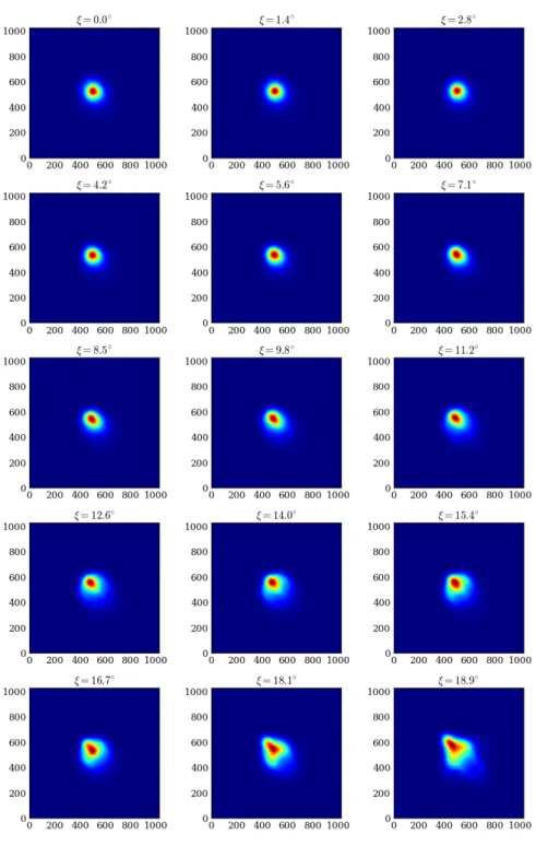
Figure 21 – Simulated PSF shapes of PLATO telescopes . . . 50
Figure 22 – Intrapixel energy distribution of PLATO PSF . . . 51
Figure 23 – Preliminary spectral response of PLATO normal cameras . . . 51
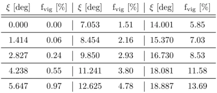
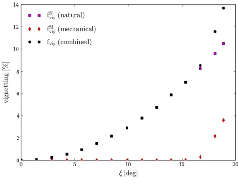
Figure 24 – Natural and mechanical obscuration vignetting of PLATO normal cameras 52 Figure 25 – Work breakdown structure of Data Processing Algorithms . . . 52
Figure 26 – Archimedean spiral used for micro-scanning strategy . . . 53
Figure 27 – Short description . . . 53
Figure 28 – Zodiacal light on the celestial sphere . . . 56
Figure 29 – Ecliptic coordinates with zero point in the Sun. . . 57
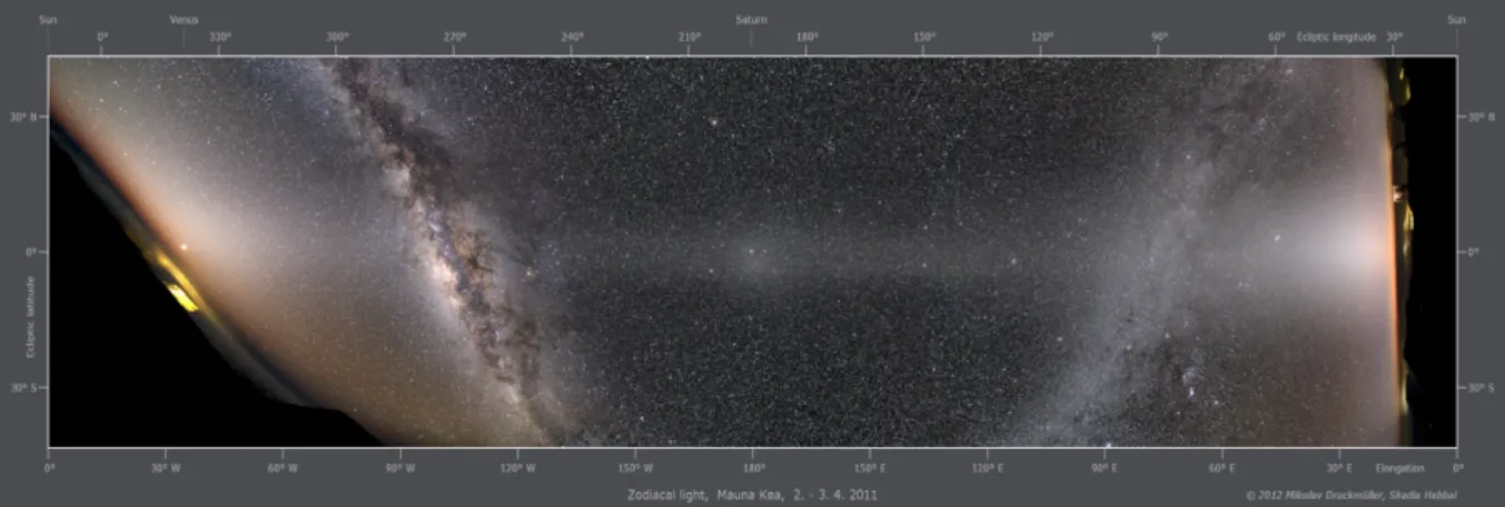
Figure 30 – Zodiacal light photo . . . 57
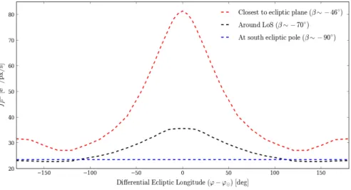
Figure 31 – Scatter plot of zodiacal light across the input field of view . . . 60
Figure 32 – Zodiacal light temporal gradient . . . 60
Figure 33 – Arbitrary camera reference frame . . . 61
Figure 34 – Projection of star position onto the focal plane . . . 62
Figure 35 – Euler angles . . . 63
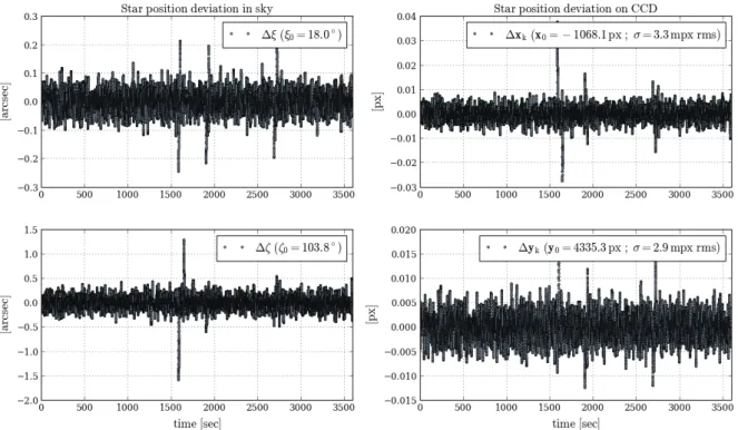
Figure 38 – AOCS nominal pointing error in the camera reference frame . . . 66
Figure 39 – Relationships between the photometric passbands V , P , and G . . . . 74
Figure 40 – Distances and differential magnitudes between contaminants and targets 75 Figure 41 – Example of input image . . . 75
Figure 42 – Noise-to-signal ratio as a function of aperture size . . . 87
Figure 43 – Shapes of photometric apertures. . . 87
Figure 44 – Nominal jitter time-series at sampling frequencies 8Hz and 0.8Hz . . . 88
Figure 45 – Noise-to-signal ratio results . . . 89
Figure 46 – SPRk results . . . 90
Figure 47 – SPRtot results . . . 90
Figure 48 – Scatter plot of NTCEgood . . . 93
Figure 49 – Statistics on transit depth and transit duration of eclipsing binaries . . 94
Figure 50 – Scatter plot of SPRappk . . . 99
Figure 51 – Histogram of the distribution of contaminant stars with SPRappk ě SPRcritk 100 Figure 52 – Fractional distribution of Nbad TCE as a function of Galactic latitude . . . 101
Figure 53 – Input image used for simulating long-term star position drift . . . 102
Figure 54 – 2D maps of aperture flux, NSR˚, and SPR as a function of the intrapixel location of target barycentre . . . 103
Figure 55 – Long-term drift simulation . . . 104
Figure 56 – Statistics on the morphology of binary masks . . . 112
Figure 57 – Schematic of double aperture photometry on board . . . 115
Figure 58 – Number of number of potential background eclipsing objects per target star . . . 116
Table 1 – Summary of PLATO mission stellar samples . . . 38
Table 2 – Summary of main payload characteristics . . . 44
Table 3 – Preliminary spectral response of PLATO normal cameras . . . 46
Table 4 – Natural and mechanical obscuration vignetting of PLATO normal cameras 46 Table 5 – Description of the parameters of zodiacal light model. . . 58
Table 6 – Coordinates of the input field line of sight . . . 59
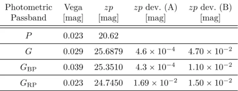
Table 7 – Zero points of the synthetic P , G, GBP and GRP photometric passbands 68 Table 8 – Predicted stellar flux entering PLATO’s normal cameras . . . 69
Table 9 – Description of the parameters of noise-to-signal ratio expression . . . 80
Table 10 – Noise-to-signal ratio degradation caused by jitter . . . 88
Table 11 – NTCEgood results (a) . . . 92
Table 12 – NTCEgood results (b) . . . 92
Table 13 – NTCEbad results (a) . . . 97
Table 14 – Nbad TCE results (b) . . . 98
1 Introduction . . . 13
1.1 Searching for potentially habitable planetary systems . . . 13
1.2 Stellar classification . . . 18
1.3 Probing stellar interior with asteroseismology . . . 21
1.4 Detecting exoplanets . . . 21
1.5 Extracting photometry from stars . . . 26
1.6 This thesis . . . 29
2 The PLATO space mission. . . 31
2.1 A brief history of the project. . . 32
2.2 Mission Consortium. . . 33
2.3 Science goals . . . 33
2.4 Science requirements . . . 35
2.5 Stellar samples . . . 37
2.6 Observation strategies and envisaged stellar fields . . . 38
2.7 Launch, orbit and science operations . . . 40
2.8 Data products . . . 41
2.9 Instrument description . . . 42
2.10 Data processing algorithms. . . 47
3 Image formation at PLATO detectors . . . 55
3.1 Zodiacal light . . . 55
3.2 The input stellar catalogue . . . 58
3.3 Determining stellar positions on the focal plane . . . 59
3.4 Satellite jitter . . . 61
3.5 A synthetic PLATO P photometric passband . . . 67
3.6 Identifying target and contaminant stars . . . 70
3.7 Setting up the imagettes . . . 71
3.8 Discussions . . . 71
4 Aperture photometry . . . 77
4.1 State of the art . . . 77
4.2 Proposed approach for PLATO P5 targets . . . 78
4.3 Photometric precision . . . 79
4.4 Confusion . . . 80
4.5 Detectability of planet transits. . . 81
4.6 Sensitivity to background false transits . . . 82
4.7 Background flux correction . . . 83
4.10 Discussions . . . 101
5 Conclusions and perspectives . . . 107
5.1 Conclusions . . . 108
5.2 Perspectives . . . 114
Bibliography . . . 121
Appendix
131
APPENDIX A Photometric performance breakdown of PLATO P5 stellar sample . . . 133Annex
135
ANNEX A Published papers. . . 1371 Introduction
The search for life beyond Earth is certainly one of the most captivating and inspiring questions in modern science. When contemplating the boundlessness of our universe, with its hundred billions galaxies composed of countless stars and planets, we might fell impelled to interrogate ourselves with a simple yet meaningful question: “Are we alone?”. It turns out that scientifically answering to this question has been proven to be one of the toughest challenges in the cohesive scientific fields of astronomy, astrophysics and astrobiology (see Caporael(2018),Galante et al. (2016)). Indeed, even with the most powerful telescopes available to date, which are sensitive to electromagnetic radiation in a wide range of wavelengths and thereby capable to probe the universe at mind-blowing distances far away from our Solar System, no clear sign or evidence of existing life beyond Earth was ever found yet.
1.1
Searching for potentially habitable planetary systems
From a scientific point of view, unveiling the secrets of the origin of life requires carefully examining the environment conditions and the physicochemical processes that favoured and sustained life. A valuable step towards that comprehension resides in searching for potentially habitable planetary systems beyond our Solar System, so that we can properly understand how these systems typically form and evolve. In this context, the concept of habitable zone gives, based on the only known life-sustaining sample (the Earth), a clue on where life as we know is (more likely) expected to be encountered.
Habitable zone (HZ), also called Goldilocks zones, may be understood as the zone around a star where the temperature is just right (i.e. not too hot and not too cold), so that liquid water can exist on the surface of a planet orbiting that star. Accordingly, the hotter a star is, the farther away and the larger will be its HZ, and vice-versa. In the literature, habitable zones are estimated based on planetary climate models such as those presented in Kasting, Whitmire & Reynolds (1993), Kopparapu et al. (2013), Shields, Ballard & Johnson (2016), Bin, Tian & Liu (2018). As represented in Figure 1, HZ sizes may be more optimistic (wider) or more conservative (narrower), depending on the considered
model. According to the conservative definition (Kopparapu et al. (2013)), the Earth is
located at the inner boundary of Sun’s habitable zone.
In a judicious way, habitable zones shall not be however strictly thought in terms of temperature only. There are other fundamental physical aspects that significantly contribute to make a planet capable to harbour life. An atmosphere (air), for example, is essential for the existence of life in a planet, because without it, there is not sufficient
pressure to keep water in liquid state, even if the planet has the right temperature. To some extent, an atmosphere also act as a protective skin against spatial objects on collision courses with a planet, by incinerating them before they can hit the planet surface. Persistent atmospheres require, in turn, the existence of sufficiently strong magnetic shields, otherwise the radiation winds emitted by a star may easily vaporize the atmosphere of a planet orbiting within its habitable zone. Hence, the conditions for the emergence and the maintenance of life are in practice much more complex than the formal definition of habitable zone might suggest. Yet, this concept still represents today our best guess on where to search for potentially habitable planetary systems.
Figure 1 – Habitable zone around main sequence stars of spectral type F, G, K, and M, as a function of the stellar temperature and the planetary orbit distance to its host star. Boundaries of HZ may be divided into optimistic (light green) and conservative (dark green) versions.
Source: Planetary Habitability Laboratory (PHL), University of Puerto Rico, Arecibo.
The first confirmed exoplanet discoveries dates from the 90’s (Wolszczan & Frail (1992), Mayor & Queloz(1995)). Yet, spatial missions dedicated to widely search for new exoplanets only started operating by the second half of the 2000’s (seeFigure 2); first, the pioneer mission Convection, Rotation and planetary Transits CoRoT (Baglin et al. (2006), Auvergne et al.(2009),Deleuil & Fridlund (2018)) from the French Space Agency (CNES),
in 2006; then the breaking though mission Kepler (Borucki et al. (2010)) from NASA, in
2009. At the present date, both CoRoT and Kepler spacecrafts are no longer operational.
In contrast, the NASA exoplanet hunter spacecraft TESS (Ricker et al. (2014)), launched
Additionally, the ESA spacecraft CHEOPS (Cessa et al.(2017)), expected to be launched by the end of 2019, will observe bright targets which are already know to host super-Earth to Neptune mass planets. The aim of this mission is to accurately determine the radii of these planets, for which the respective masses have already been obtained by ground-based spectroscopic surveys.
Figure 2 – Timeline of exoplanet missions.
Source: ESA.
Since the first detections, a substantial number of exoplanets were discovered and confirmed. To date, this number adds up to 4,009 exoplanets according to the NASA Exoplanet Archive1. However, most of these planets (seeFigure 3) are either much closer to their host star or much more massive when compared to the Earth (or both). Hence, even considering the important advances occurred in the matter of the exoplanet search science over the last two decades, which allowed us to discover thousands of new exoplanets, we are still incapable to assert if there are effectively other planets like our Earth, let alone how many of them and what type of star they orbit.
Besides, we cannot state either that Earth-like planets are simply rare, so that we can consider that we live in an “outlier” planet. The reason is that most of the stars around which the planets of Figure 3were detected are, typically, relatively faint (see Figure 4). In other words, the photometry of these stars do not have sufficient signal-to-noise ratio (SNR) allowing Earth-sized planets – orbiting within their habitable zone – to be detected
and accurately characterized in terms of mass and radii. Therefore, the fact that we have not found yet a planet like our Earth could be owed to the fact that we have still not observed a sufficiently large sample of bright stars.
Figure 3 – Confirmed exoplanets to date (4,009 in total).
The only spatial mission – within the next few years – that is qualified to find new exoplanets, TESS, will not be capable of making significant impact on the detection and characterization of Earth-sized planets, except for those orbiting coolest M-type stars, for which the mission is mostly designed for. Therefore, a clear gap exists when it comes to find Earth-like planets orbiting the habitable zone of Sun-like stars.
Figure 4 – Magnitude of the stars hosting the planets ofFigure 3.
Source: Nasa Exoplanet Archive.
In this respect, the ESA planet-hunter spatial mission PLATO appears as a promising solution to cover this gap. Expected to start operating in 2026, the PLATO mission takes place in the context of ESA’s long-term planning for space science missions called Cosmic Vision. This Program was conceived to address fundamental scientific questions related to the origin of our Universe and the physical laws that drives it, the formation of planetary systems and the origin of life. In that thematic, PLATO aims at
investigating three major questions (ESA(2017)):
• How do planets and planetary systems form and evolve?
• Is our solar system special or are there other systems like ours? • Are there potentially habitable planets?
To do it, PLATO builds upon the well-proven techniques that allowed the success of its predecessors CoRoT and Kepler missions. That is the transit method for detecting exoplanets, along with radial velocity spectroscopy follow-up from the ground, and the analysis of stellar oscillations via asteroseismology for characterizing their host stars. However, PLATO stands out from any other mission of its category in the sense that it is being specially designed to not only discover but also characterize (in terms of mass, radii, and density) Earth-like planets orbiting within the habitable zone of bright main-sequence Sun-like stars. Moreover, by also focusing on constraining stellar ages PLATO might be capable of determining changes in planetary systems architecture over the time, such as the dependency of exoplanet frequency with main-sequence stellar age (Veras et al. (2015)). Ultimately, PLATO is expected to provide enough elements allowing us to finally determine with accuracy whether Earth-like planets exist or not, how many of them and which type of star they orbit (Baudin & Damiani (2019)).
The work presented in this thesis takes place in the preparation phases of PLATO space mission, more precisely in the development of data processing algorithms.
1.2
Stellar classification
Simply stated, a star is a spherical celestial body of plasma (i.e. super hot gas) whose formation is resulted from the gravitational collapse of molecular clouds of cold gas – mostly composed of hydrogen and helium – that are present in the interstellar medium.
As the clouds accumulate, they form a central region – called protostar (see Campante,
Santos & Monteiro (2018)) – that becomes denser and hotter than the outer regions. At a certain point owing to the increasing pressure, the protostar temperature becomes high enough so that fusion reactions starts to take place in its core, thereby causing hydrogen to be converted in helium. Such splendid moment characterizes the birth of a star. From that point on, the star’s life expectancy is determined by the nuclear time-scale associated to its total fusing hydrogen mass (fuel). Hence, the more massive the star, the quicker it consumes hydrogen, thereby resulting in shorter lifespan, and vice-versa. The amount of gas and dust material orbiting a young star, known as the circumstellar disc, may also accumulate away from that star to form planets (Fortier et al.(2012)).
The different evolutionary states of a star throughout its lifetime (see schematic in Figure 5) are commonly represented using a Hertzsprung–Russell diagram (HRD), which displays the correlation between stellar surface luminosity and effective temperature. An
example of HRD produced with stars observed by Gaia (Gaia Collaboration et al., 2016)
is shown in Figure 6, with stellar luminosities normalized by that of the Sun. The diagram clear evidences that most of the stars found in our sky belongs to the main sequence branch, which is consistent with the fact this corresponds to the longest phase in stellar evolution. Effective temperature and abundances of heavier elements than hydrogen or
helium (i.e. metallicity) defines the spectral classification of a star, which is designated with the letters O, B, A, F, G, K, and M (in order of decreasing temperature). Besides, stars are also subdivided according to their luminosity class (Cox(2002)): I (supergiants), II (bright giants), III (giants), IV (subgiants), and V (dwarfs or main sequence). Moreover, the effective temperature of a star has a direct link with the colours form the electromagnetic spectrum. Accordingly, coolest stars look redder and hotter stars look bluer.
Figure 5 – Stellar evolution scheme.
Source: Encyclopedia Britannica, Inc.
Our Sun is a main sequence (dwarf) yellow G2V-type star with effective temperature of about 5,800K. Its total life expectancy is about 10 billion years (Campante, Santos & Monteiro (2018)). M-type stars of the main sequence branch have a fraction of the Solar mass, so they are relatively faint and cool (À 3, 500K) stars, and have an estimated lifespan of the order of trillion years (Adams, Graves & Laughlin(2004)), thereby extremely longer than the age of the Universe (about 13.8 billion years). In other words, such stars can be considered relatively young in their evolution. Also, this class of star is the most commonly encountered in the Milky Way (Henry, Kirkpatrick & Simons (1994)). Lastly, the earlier mentioned red giants are relatively cool (K or M) spectral type stars, but much brighter than our Sun as previously explained.
In terms of planetary formation, latest observations evidenced the existence of a direct correlation between stellar metallicity and the occurrence of gas giants (e.g. Neptune-and Jupiter-like) planets (Fischer & Valenti (2005), Johnson et al. (2010)), which however do extend to small ones, more specifically for those whose radius is smaller than four times that of the Earth (Rp ă 4R‘). Furthermore, analysis based on Kepler data indicate that
terrestrial or smaller planets are not constrained by environment metallicity, suggesting therefore that such category of planets might be relatively common across our Galaxy (Buchhave et al. (2012)).
Figure 6 – Hertzsprung–Russell diagram of stars observed with Gaia.
1.3
Probing stellar interior with asteroseismology
In astrophysics, stellar physics is the science of studying the internal structure of stars and how these evolve throughout time, which involves understanding several physical and chemical notions such as hydrodynamics, thermonuclear reactions, radiative transfer, quantum mechanics and general relativity. Although there exist no actual technology capable to directly explore the interior of stars (i.e. with physical instruments inside them), their composition, functioning and evolution can be fairly well understood thanks to the great advances – achieved in the last few decades – in the research field of asteroseismology (Baglin et al. (2006), Aerts, Christensen-Dalsgaard & Kurtz (2010), Mosser & Miglio (2016), Campante, Santos & Monteiro (2018)).
Asteroseismology is a branch of stellar physics that allows one to probe the internal structure of stars by studying the seismic waves that propagate inside them, as analogous to the approach used in terrestrial seismology. In other words, in the same way as analysing the seismic waves generated by earthquakes provides information about Earth’s interior (temperature, pressure, rocky composition etc.), analysing the oscillation modes of a star provides us key information about its internal physical properties and dynamics (e.g. mean density, chemical composition, rotation etc.).
Stellar oscillations cause periodic variations in star brightness that exhibit regular
patterns in the frequency domain (see Figure 7). These patterns, which carry important
information on specific characteristics of the stellar structure, can be measured by a sufficiently sensitive (high signal-to-noise ratio) photometer. For example, the average large separation ∆ν between larger peaks contains information about stellar mean density, whereas the small separations δν carry finger prints of the chemical composition in the stellar core, which can be used to infer the amount of hydrogen in it and ultimately the corresponding stellar age. Besides, inversion techniques (Reese et al. (2012), Buldgen et al. (2015)) can be applied to several observed and measured oscillation mode frequencies to determine e.g. the internal rotation profile of the star. In particular, stellar rotation may impact on both internal structure and evolution of stars (Gehan (2018)), including their ages (Lebreton & Goupil (2014)).
Asteroseismic studies can be performed through Doppler spectroscopy from ground-based observations. However, since measuring stellar oscillations requires sufficiently high duty-cycle and low-noise observations, better results in asteroseismology are obtained from spectral analysis of photometry signals extracted from stars with space-based surveys.
1.4
Detecting exoplanets
The exoplanet search science counts on a variety of detection methods, two of which are widely employed: the transit photometry and the radial velocity. Indeed, among
Figure 7 – Power density spectrum of the Sun.
Source:Campante, Santos & Monteiro (2018).
all the confirmed planets of Figure 3, which were detected using ten different methods,
transit photometry and radial velocity account respectively for „ 77% and „ 19%, that is „ 96% altogether, of these discoveries. The following sections provide brief descriptions of both methods. This thesis is focused in the science and usage of the transit method, on which the PLATO mission relies for detecting exoplanets. A complete list with detailed descriptions of planet detection techniques is provided inPerryman (2018).
1.4.1 The transit photometry method
The principle of the transit photometry method is simple: a planet passing in front of (eclipsing) its parent star (see representation inFigure 8) causes an apparent dip in its brightness whose amplitude is proportional to the second power of the planetary-to-stellar radius ratio.
Accordingly, dips produced by larger planets such as gas giants are much easier to detect than those produced by terrestrial planets. For example, a Jupiter-like planet orbiting a Sun-like star causes a stellar brightness dip (transit depth) which is about two orders of magnitude larger than that produced by an eclipse of an Earth-like planet
Figure 8 – Representation of transit photometry method.
Source: ESA.
orbiting that same type of star. In contrast, another important aspect that significantly influences in the detection capabilities of transit method is the angle between the observer’s line of sight and the planetary orbital plane. Assuming planets with randomly oriented orbits, their corresponding visibility angles in the sky represent a small fraction of the celestial sphere, decaying exponentially with respect to the planetary-to-stellar distance. For example, terrestrial planets orbiting at 1 AU distant from Sun-like stars produce transits that are visible from only „ 0.46% of the celestial sphere. For a Jupiter-like planet orbiting at 5.2 AU distant from Sun-like stars, that visibility drops to only „ 0.09% (Bozza, Mancini & Sozzetti (2016)), that is five times lower visibility probability (although the transit depth produced by such planet is significantly easier to detect as explained before). In any case, the intrinsic low probability of having a planet transit visible in the sky shows that building a statistically significant sample of exoplanets requires observing several thousands of stars over at least a few years.
The first known exoplanet to be discovered with transit photometry dates from the early 2000’s. The authors of this discovery reported a transiting object causing a 1.2% transit depth in its host star’s light curve, giving an estimated planetary radius of about 1.3 Jupiter radii. Later radial velocity measurements from that object suggested it to be a planet with around 90% of the Jupiter mass in an orbit at only 0.023 AU distant from the host star (Konacki et al.(2003)). Hence, given its proximity to the parent star and physical similarity to Jupiter, this planet enters in the category of planets called “hot Jupiters”. Hot Jupiters are virtually the easiest planets to detect since they are very
large and close to the host star, thereby producing large transit depths and having large fractions of the celestial sphere through which observers can see it. Not surprisingly, there is a relatively high occurrence of hot Jupiters among the confirmed exoplanets shown in Figure 3. Terrestrial planets around Sun-like stars, in contrast, are very tough to be detected, in particular because of the strong requirements in terms of noise performance. Indeed, detecting such category of planets requires photometric precisions of the order of a few dozens parts-per-million (ppm), which requires therefore observing sufficiently bright targets.
1.4.2 The radial velocity spectroscopy method
A planet orbiting its host star causes the latter to wobble around the centre of mass of the system formed by both celestial bodies. From an observer’s point of view, the light it receives from the wobbling star periodically shifts in wavelength over the time, going redder when it moves away and going bluer when it moves towards the observer (see representation in Figure 9), analogously to the change in wavelength that occurs in sound waves owing to the Doppler effect.
The radial velocity (or Doppler spectroscopy) method consists therefore in measur-ing the tiny („ 10´4Å) wavelength shift in the light from a wobbling star, which is then
translated into a corresponding stellar radial velocity projected in the direction of the radius connecting the star and the observer. That velocity depends on both star and planet masses. Since the former can be obtained from the stellar oscillation analysis through asteroseismology, the mass of the planet can finally be determined.
Radial velocity has shown to be a powerful method for detecting and characterizing masses of exoplanets. However, the main drawback of this method is the fact that it can only provide unambiguous mass estimations if the inclination angle between the observer’s line of sight and the orbital plane of the planet is known. Otherwise, the method is limited to estimate only the planet’s “projected mass” in the direction of the observer’s line of sight, that is the minimum planet mass (Campante, Santos & Monteiro (2018)).
1.4.3 False transit signatures
Planets orbiting stars are not the only astrophysical sources capable of producing transit-like signals in light curves. Binary stars, which are known to exist since William Herschel back in the 1700’s, can naturally produce transit dips as well. Therefore, if one looks at finding new exoplanets, then one should be capable of distinguishing legitimate planetary transits (i.e true positives) from those which are not (i.e. false positives).
In the context of the Kepler mission, a concept was created to designate statistically significant transit-like signatures marked for further data validation: the threshold crossing events (TCE) (see e.gTwicken et al. (2018)). Each of these events become a Kepler Object
Figure 9 – Representation of radial velocity (Doppler spectroscopy) method.
Source: NASA.
of Interest (KOI) (i.e. a planet candidate) which shall be subjected to proper vetting process in order to check whether they are true planets or not.
There are principally four astrophysical phenomena (Figure 10) capable of producing statistically significant transit-like signatures (Bozza, Mancini & Sozzetti (2016)):
1. Planets orbiting stars;
2. Grazing eclipsing binaries with similar mass and size;
3. Medium- or high-mass stars with low-mass (e.g. red dwarf) stellar companions; 4. Blended eclipsing binaries.
The latest three are examples of false positives. During vetting process, some of these false planet transits can be quickly identified by looking at their shape. For example, grazing stellar binaries produce transit signals that are V-shaped, whereas legitimate planet transits are U-shaped. Besides, a transit produced by eclipsing binaries with different effective temperatures is inevitably colour-dependant, which is naturally not the case of a true planet transit. Furthermore, eclipsing binaries periodically present two distinct transit depths, since both stars of the system are eclipsed alternately.
A blended eclipsing binary system consists of a isolate foreground (target) star, i.e. a star from which we are interested to extract photometry from, with a background
Figure 10 – Astrophysical phenomena producing transit-like signatures.
Source:Bozza, Mancini & Sozzetti (2016).
eclipsing binary (BEB) companion. Their separation in the sky is small enough so that the BEB can pollute the photometry of the target star on the detector of a photometer.
For the Kepler mission, Bryson et al. (2013) developed methods for detecting
background false positives based on changes in the star image that occur during a transit. The authors found that, at low Galactic latitudes, background false positives account for near 40% of all Kepler transit-like signals.
1.5
Extracting photometry from stars
Analysing stellar oscillations through asteroseismology and detecting exoplanets with transit photometry requires extracting light curves from targets stars. One of the key point in this task consists in properly quantifying the amount of signal and noise that is embedded in the light curve. Since stars emits photons following a Poisson distribution, the photometric flux signal measured from a star has variance σ2 and mean f such that f “ σ2.
Accordingly, the SNR of the raw stellar flux is SNR “ f {σ “ f {?f “?f , i.e. equal to the square root of the mean flux. Higher SNR requires therefore a proportionally higher average flux, which can be obtained by augmenting the interval during which photons from the target star are collected. In contrast, measuring the total photon count from a star necessitate a detector – typically a charge couple devices (CCD) in spatial applications – which counts photons in discrete packages (pixels) that contribute, each, with additional noise in the photometry. That amount of extra noise depends on the quality of the detector and on the Point Spread Function (PSF) of the optics that drives the (point source) flux
from a star towards a given position of the detector. The more distorted the PSF, the larger the number of pixels required to register the star signal on the detector, thereby the greater is its noise contribution in the photometry. Furthermore, sources of photon flux from the sky such as contaminant stars and scattered zodiacal and Galactic lights also contribute to the total noise embedded in the photometry extracted from a star.
In all such context, extracting high precision light curves from stars is far from being a straightforward task. While several photometry extraction methods exist in the literature, they are all essentially derived from two major techniques: PSF fitting and aperture photometry. We provide a general description of both methods in the following sections.
1.5.1 PSF fitting photometry
The PSF fitting method consists in fitting a PSF-based image model of a star to its measured one, such as to minimize the following functional:
χ2 “ ÿ i,j ´ Ii,j´ ˆIi,j ¯2 σ2 i,j , (1.1)
where Ii,j corresponds to the measured star image, ˆIi,j the modelled star image and σi,j2
the variance of the measured flux at pixel coordinate pi, jq. The modelled star image ˆIi,j
can be defined as (Deheuvels & Ballot (2019)):
ˆ
Ii,j “ a ˆ Pi,jpxc, ycq ` b, (1.2)
where ai,j is the stellar flux at pixel coordinate pi, jq, bi,j is the background flux at pixel
coordinate pi, jq, and Pi,jpxc, ycq is a PSF description at pixel coordinate pi, jq with centroid
coordinate pxc, ycq. Hence, the free parameters of the fit are xc, yc, a, and b.
The essential objective of this method is to determine, at pixel level, what are the contributions of the target star flux and the background flux to each pixel of the measured star image Ii,j. Going further, this method can be refined to include contributions from
contaminant stars present in the star image scene. By doing so, one is then capable to optimally detach the average flux of the target star from that of contaminant sources and the diffuse background light. Moreover, the PSF fitting technique has also the advantage of providing relative accurate („ 10´2 pixel) estimates on the centroid position of stars
and is less sensitive to satellite jitter and long-term stellar position drift. In contrast, since – in real world scenario – uncertainties on the knowledge of the instrument PSF always
1.5.2 Aperture photometry
In aperture photometry, each light curve sample is generated by integrating the target flux over a limited number of pixels which shall be appropriately selected to maximize the scientific exploitability of the resulting time-series light curve.
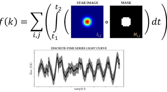
Figure 11 – Schematic of aperture photometry method to produce a time-series light curve. The symbol “˝” stands for the Hadamard (element-wise) product applied between the (generic) star image Ii,j and the (generic) aperture Mi,j, both of
identical shape.
Source: author, with plot fromSamadi et al. (2019).
Mathematically, the aperture photometry method can be described as
f pkq “ÿ i,j ˆżt2 t1 pIi,j˝ Mi,jq dt ˙ . (1.3)
In the above expression, Ii,j is a square matrix of indexes i and j representing the image of
a star; Mi,j is a square matrix of identical shape of Ii,j representing an aperture (mask); t is
the time in continuous domain; pt2´ t1q ą 0 is the detector integration time; k represents
the index of a single light curve sample; and f pkq if the photometric flux relative to the light curve sample k. The symbol “˝” stands for the Hadamard (element-wise) product applied between the star image Ii,j and the aperture Mi,j. A discrete-time series light
1.6
This thesis
The PLATO mission is expected to observe up to one million stars, depending on the final observation strategy. In contrast, transmitting to the ground individual images from each of these stars at sufficiently short cadence for further processing requires prohibitive telemetry resources. Hence, for a substantial fraction of the targets, an appropriate in-flight data reduction strategy (prior to data compression) needs to be executed. For that, the most suitable encountered solution consists in producing their light curves on board.
In view of its acknowledged high performance and straightforward implementation, mask-based (aperture) was adopted as photometry extraction method to produce light curves in flight. In such context, the present work unfolds the development carried out for defining the optimal collection of pixels (i.e. the aperture Mi,j,Equation 1.3) for extracting
photometry on board from a significant fraction of the PLATO targets. Compared to the common approaches found in the literature to determine aperture shapes, this work brings a novel perspective through which greater importance is given to the problematic of background false positives (subsubsection 1.4.3). The major motivation for that is to provide ways of eliminating astrophysical false positives as early as possible in the planet discovery process. This is justifiable since although effective techniques exist for detecting false positives (e.g. Bryson et al. (2013)) from the observations, in most cases the vetting process of planet detections usually requires ground-based confirmations via radial velocity measurements that consume (costly) telescope time. Accordingly, using such infrastructure to identify false positives – that could be earlier rejected by the time of the detection – represent significant waste of money and time. Furthermore, the vast majority of light curves produced in flight will not have pixel data available on the ground for the identification of false positives. The main challenge involved in this work relies on the fact that it needs to propose an aperture photometry solution delivering sufficiently high photometric precision to be in agreement with the science requirements defined for the PLATO mission, and sufficiently low sensitivity to false planet detections; all that for a huge number of targets with the limited CPU and memory resources available in the spacecraft payload.
The following of this document2 is organized as follows: Chapter 2 provides an
overview of the PLATO mission including its science objectives and requirements, envisaged observation strategies and data products. This chapter also describes the main payload characteristics, including instrument point spread function (PSF), spectral response, and
noise. Chapter 3 gives details on the extracted data from the adopted input catalogue
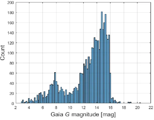
(Gaia DR2). That information is used to build synthetic input images, called imagettes, to characterize the performance of aperture photometry. A synthetic PLATO P photometric
2 This document uses the LATEX typesetting package abnTeX2 for technical and scientific documents.
passband, calibrated on the VEGAMAG system, is derived to avoid the inconvenience of having colour dependency when estimating stellar fluxes – at detector level – from visual magnitudes. Colour relationships with Johnson’s V and Gaia G magnitudes are thus provided. Moreover, an expression is derived to provide an estimation on the intensities
of zodiacal light entering each PLATO telescope.Chapter 4 describes the methodology
applied to find the optimal aperture model to extract photometry from stars in P5 sample. Three models are tested, including a novel direct method for computing a weighted aperture providing global lowest NSR. The chapter ends by showing comparative results between all aperture models with respect to their sensitivity in detecting true and false planet transits. Finally,Chapter 5concludes with discussions on the presented results and perspectives/open issues for future work.
2 The PLATO space mission
PLAnetary Transits and Oscillations of stars (PLATO)1 (Rauer et al. (2014)) is
a space mission from ESA whose science objective is to discover and characterize new extrasolar planets and their host stars. Expected to be launched by the end 2026, this mission will focus on finding photometric transit signatures of Earth-like planets orbiting the habitable zone of main-sequence Sun-like stars. Thanks to its instrumental concept comprising multiple telescopes covering a very large field of view, PLATO will be able to extract long duration photometry from a significantly large sample of bright stars at very high photometric precision, allowing it to accurately characterize planetary and stellar parameters such as mass, radii, density and age.
Figure 12 – Artist’s impression of PLATO spacecraft.
Source: OHB System AG.
In this chapter, we provide an overview of the very foundation on which the PLATO mission and the present work are built. We start by giving a brief history of the project until its current development stage, then we move along the top science goals of the mission and derived requirements, covering the aspects of observational constraints and strategies. Next, a description of the instrument concept is given, including a summary of the main payload characteristics containing all the instrument parameters used in this work. We also provide a overview of the science data processing pipeline, in which context the present work takes place.
The work presented in this chapter is partially based onMarchiori et al.
(2019). In-flight photometry extraction of PLATO targets: Optimal apertures
for detecting extra-solar planets, A&A, 627, A71.
2.1
A brief history of the project
The PLATO mission was first proposed to ESA by a broad group of European scientists headed by Dr. Claude Catala (Paris Observatory), in response to the Call for (M-class) mission proposals of Cosmic Vision 2015-2025 released on March of 2007. From
a total of 52 proposals, PLATO was pre-selected along with five other projects.
In June 2011, PLATO successfully completed phase A (feasibility evaluation), after having gone through assessment and definition studies which involved two independent industries to investigate the mission concept, and a Consortium of research Institutes and Universities to study the payload. The proposal however was not selected for the M1 or M2 launch opportunities as originally planned. Shortly after its non-selection, PLATO candidature was re-submitted for the M3 launch opportunity with renewed science case and mission design. One of the major changes in the new proposal was the transfer of the leading role from France to Germany, with Prof. Heike Rauer (DLR) taking place as PLATO Principal Investigator. On February 19th 2014, PLATO was selected by ESA for the M3 launch opportunity in 2022–2024.
After the selection, the mission entered in phase B (preliminary definition), this time involving three concurrent industrial contractors (Airbus Defence and Space, OHB System AG, and Thales Alenia Space) for designing the spacecraft. After being subjected to a thorough independent review at ESA, the new PLATO Science Management Plan was approved by the ESA Science Programme Committee in June of 2016. The approved plan included a (revised) baseline payload configuration comprising 26 telescopes with nominal science operations of fours years (plus a verified in-orbit lifetime of 6.5 years and eight years of consumables). The ESA Science Programme formally adopted the PLATO mission in June of 2017. In May of 2018, OHB System AG – a subsidiary of Bremen-based space and technology group OHB SE – was selected as the prime contractor of PLATO. The prime is responsible for constructing the spacecraft platform (which includes the main
satellite structure, the propulsion system, the solar panels, the attitude and orbit control system, among others features) and integrating it with the payload.
The mission is currently in end of phase B and shall be ready to start phase C (detailed definition and implementation) by end 2019. A recent important milestone for the mission was the delivery to ESA of a first batch of 20 charge-coupled devices (CCDs) in mid March of 2019.
2.2
Mission Consortium
The PLATO Mission Consortium (PMC) regroups several hundreds of scientists from almost all ESA Member States, including a few scientists from the United States and Brazil. The PMC is lead by the project Principal Investigator and is responsible for building, integrating, verifying, calibrating and delivering the PLATO payload to ESA. The payload subsystems include camera optical elements and detectors, flight hardware and software, electronics, as well as the pipeline algorithms and modules to generate high level scientific data products.
The PMC structure (Figure 13) includes the PLATO Data Centre (PDC) and the PLATO Science Management (PSM) teams. The PDC team is responsible for developing methods and tools for analysing, validating and calibrating the data collected by the spacecraft. The PSM provides scientific specifications for the PDC, specifies the PLATO input catalogue and organises preparatory and follow-up observations.
2.3
Science goals
The PLATO mission is in synergy with the fundamental questions that drives the ESA Cosmic Vision Program. Accordingly, the core design of the mission was established with top level science goals that can be broken down into the following specific objectives
(PLATO Study Team (2017)):
1. Determine the bulk properties (mass, radii, and mean density) of planets in a wide range of systems, including terrestrial planets in the habitable zone of solar-like stars;
2. Study how planets and planet systems evolve with age; 3. Study the typical architectures of planetary systems;
4. Analyse the correlation of planet properties and their frequencies with stellar param-eters;
5. Analyse the dependence of the frequency of terrestrial planets on the environment in which they formed;
Figure 13 – Overview of PLATO PMC structure.
Source: Dr. Heike Rauer, principal investigator of the PLATO Mission Consortium.
6. Study the internal structure of stars and how it evolves with age2;
7. Identify suitable targets for spectroscopic follow-up measurements to investigate planet atmospheres.
The above science goals should allow PLATO – among other aptitudes – to better constrain planet formation and evolution models, identify potential candidates for habitable planets, improve stellar models and ages in general, correlate planet parameters with stellar properties and correlate planet occurrence frequency with environment.
To achieve its science goals, the PLATO mission aims at building and characterizing a statistically significant sample of planets down to Earth-size orbiting within the habitable zone of bright main sequence F, G, K Solar-type stars and M-stars. To accomplish it, the mission builds upon the transit method for detecting exoplanets, spectroscopic radial-velocity follow-up and TTVs measurements for determining exoplanet mass, and asteroseismology to determine masses, radii and age of exoplanet host stars.
Following that strategy, PLATO should be capable of delivering seismic charac-terization of a large sample of bright stars across the HR diagram (PLATO Study Team
(2017)). Moreover, PLATO will be the first mission of its category being capable of provid-ing a significant sample of (super) Earth-like planets orbitprovid-ing within the habitable zone of Sun-like stars (Goupil(2017)). Furthermore, coupling accurate parameters of planets with those from their (bright) host stars should provide a consistent census of exoplanetary systems neighbour of our own Solar System.
2.4
Science requirements
We present here below a non-exhaustive list containing the major scientific require-ments established for both asteroseismology and exoplanet search sciences of the PLATO mission, derived from the science goals described in the previous section. PLATO shall be
capable of (PLATO Study Team (2017),ESA (2017), Goupil(2017)):
• detect a planet orbiting a G0V star with an orbital period of one year (this is roughly equivalent to being capable of detecting an Earth-like planet orbiting a Sun-like star at a distance of 1 AU);
• determine – with accuracy better than 2% – radius of G0V stars as bright as V “ 10; • determine – with accuracy better than 15% – mass of G0V stars as bright as V “ 10; • determine – with accuracy better than 10% – ages of G0V stars as bright as V “ 10; • detect and characterize terrestrial planets orbiting dwarf and sub-giants stars brighter then V „ 8 and of spectral type F5 to late-K at distances including the habitable zone of such stars;
• provide dual photometric band information for stars brighter than V „ 8;
• detect planets orbiting dwarf and sub-giants stars of spectral type F5 to late-K at distances including the habitable zone of such stars;
• detect terrestrial3 planets orbiting M-dwarf stars at distances including the habitable zone of such stars;
• determine – with accuracy better than 3% – radius of detected planets down to Earth-size orbiting G0V stars as bright as V “ 10;
• determine – with accuracy better than 2% – planetary-to-stellar radius of detected planets down to Earth-size orbiting G0V stars as bright a V “ 10;
3 A terrestrial planet is understood herein as being a planet whose radius R
p and mass Mp satisfy
• deliver photometric data allowing to determine – through radial velocity measure-ments and with accuracy better than 10% – mass of terrestrial planets orbiting G0V stars;
• deliver photometric data allowing to determine – with precision of the order of 0.1 µHz for main sequence stars – frequencies of normal oscillation modes above and below the mode with the maximum amplitude;
• observe between 10% and 50% of the sky with observation durations of at least two months;
• sustain in-orbit nominal science operations during at least four years.
The above science requirements translate – at instrument level – into noise
require-ments (seeFigure 14) which can be summarized as follows
(A) the residual errors from systematic effects in the light curves of stars brighter than V „ 10 must be limited to two thirds of their photon noise;
(B) The item (A) above must hold within the frequency range comprised between 20 µHz and 40 mHz;
(C) The total random noise of stars brighter than V „ 10 must be limited to 34 ppm hr1{2.
(D) Noise requirements must be assured in the wavelength range between 500nm and 1000nm (visible and near infrared domains).
Satisfying the requirement (A) ensures that the total random noise in the light curve of a star brighter than V „ 10 is dominated by its photon noise.
The frequency range of requirement (B) includes the time-domain interval comprised between a few minutes for the detection stellar oscillations and a few hours for the detection of planetary transits.
Satisfying the requirement (C) ensures that the oscillation modes of Solar-type stars can be identified, and that Earth-like planets orbiting in the habitable zone of Sun-like stars can be detected and their planetary-to-stellar radius characterized with accuracy
better than 2% (ESA (2017)).
The requirements (A), (B), (C), and (D) altogether also work as drivers for linking science and engineering requirements (e.g. spacecraft pointing error, thermal control, electronics, spectral range etc.).
Figure 14 – Random noise requirements at instrument level.
Source: PLATO Study Team (2017).
2.5
Stellar samples
To achieve the science requirements, the target stars of the PLATO mission are categorized into four distinct samples (see Table 1), namely P1, P2, P4, and P5, following a criterion of scientific priority.
The Sample P1 represents the core science of the mission and holds therefore the highest priority. It is composed of dwarf and sub-giants stars of spectral type between F5 and K7, and visual magnitude V À 11. Since these stars are relatively bright and have images acquired at 25 seconds cadence, they will have very high photometric precision (À 50 ppm hr1{2). As a consequence, ground-based radial velocity follow-up is expected to
be more effective for this stellar sample.
The Sample P2, second in the order of priority, contains the brightest stars (V À 8.2) to be observed by the mission. Since their photometric fluxes exceed the saturation limit of the detectors of the normal cameras, their photometry will be extracted with the fast cameras, which have shorter image acquisition cadence (2.5 seconds). The spectral type of the stars in this sample is the same as that of P1 targets.
The Sample P4, third in the order of priority, regroups M-type dwarf stars with V À 16. Because these stars are cooler than those of the other samples, their habitable zones are closer. Therefore, the planets of interest orbiting these stars have shorter orbital periods, typically on the order of a few weeks.
Lastly, the Sample P5 includes a massive number (ą 245, 000) of F5 to late-K dwarf and sub-giants stars with visual magnitude in the range 8 À V À 13. This sample aims to generate large statistical information on planet occurrence rate and systems evolution. For comparison, the Kepler and TESS missions – of the same category of PLATO – were
designed to survey, in nominal terms, about 150,000 (Borucki et al. (2010)) and 200,000
(Ricker et al. (2014)) targets, respectively.
Table 1 – Summary of PLATO mission stellar samples.
Description Sample P1 Sample P2 Sample P4 Sample P5
Number of stars ě 15, 000 ě 1, 000 ě 5, 000 ě 245, 000
Spectral type F5 to K7 F5 to K7 M F5 to late-K
Magnitude in V band À 11 À 8.2 À 16 À 13
Cadence of 25 seconds 2.5 seconds 25 seconds 25 seconds
image acquisition
Data type images images images light curves
(centroids @50 sec for 5% of the targets) (images @25 sec for at least 9,000 targets)
Data sampling 25 seconds 2.5 seconds 25 seconds 600 seconds
(50 seconds for 10% of the targets)
Source:ESA(2017).
Within PLATO’s mission design, light curves will be produced on board exclusively for the targets of the Sample P5. For all other stellar samples, which are primarily composed of the brightest targets, the photometry will be extracted on-ground from individual images downlinked from the spacecraft, thereby following the same principle as that of Kepler and TESS targets.
2.6
Observation strategies and envisaged stellar fields
To achieve the science requirements, the PLATO spacecraft shall be capable of carrying out uninterrupted long duration (few months to several years) photometric stellar observations of a very large sample of (bright) targets at very high photometric precision.
Considering a nominal mission duration of four years, two observation scenarios are considered for PLATO. The first consists of two long-duration (2+2 years) observation phases (LOP) with distinct sky fields. The second consists of a single LOP of three years plus one step-and-stare operation phase (SOP) of one year (i.e. a (3+1 years) observation configuration), covering multiple fields lasting a few months each.
Mission design constraints require the LOP fields to have absolute ecliptic latitude and declination above 63˝ and 40˝, respectively. Under such conditions, two LOP fields
are actually envisaged: a southern PLATO field (SPF) centred at Galactic coordinates l “ 253˝ and b “ ´30˝ (towards the Pictor constellation) and a northern PLATO field
(NPF) centred at l “ 65˝ and b “ 30˝ (towards the Lyra and Hercules constellations and
also including the Kepler target field).
An illustration containing the locations of both SPF and NPF is shown inFigure 15, as well as the possible locations of the SOP fields. The definite pointing coordinates of the PLATO target fields will be defined two years before launch.
Figure 15 – Sky coverage in Galactic coordinates of PLATO’s provisional SPF and NPF long-duration LOP fields, including the possible locations of the short-duration SOP fields (STEP 01-10). The illustration also shows some sky areas covered by the surveys: Kepler (red), Kepler -K2 (green), TESS (Continuous Viewing Zones-CVZ; yellow) and CoRoT (magenta).
Source: courtesy of Valerio Nascimbeni (INAF-OAPD, Italy), on behalf of the PLATO Mission Consortium. This image is front page of A&A’s Volume 627 (July 2019).
To give an idea of the potential of PLATO observations in the matter of exoplanet detections, with an observation baseline of 2+2 years, the estimated planet yield from stars brighter than V „ 13 is of the order of 4, 600 planets (all sizes and orbital periods comprised). This represents more than the total number of discovered exoplanets to date. Yet, if a mission extension of two more years is granted, the total planet yield – with an observation baseline of 3+1+2 years – might achieve expressive „ 13,000 planets from
stars brighter than V „ 13 (ESA (2017)). A mission extension of at least two years is
possible considering that the spacecraft is designed for a (nominal) in-orbit operation lifetime of 6.5 years and will carry consumables for 8 years.
2.7
Launch, orbit and science operations
Uninterrupted long duration and high photometric precision observations as those specified for PLATO requires a sufficiently stable spatial environment. That is, the satellite must be placed into an orbit where it can keep its sight permanently turned to the target field without any viewing obstruction, and preferably with (relative) high thermal stability.
Low-Earth orbits suffer from important flux gradients of energetic particles (e.g. due to the South Atlantic Anomaly (Baglin, Chaintreuil & Vandermarcq(2016), Nasuddin, Abdullah & Hamid (2019)), high levels of scattered Sun-light reflected by the Earth, frequent observation interruptions, and strong thermal variations at timescales of minutes to hours. Hence, the PLATO spacecraft will be placed into a (sufficiently away from the Earth) Lissajous orbit4 around the L2 Lagrangian point (Figure 16). The L2 point, which is about 1.5 million kilometres (0.01 au) beyond the Earth orbit distance with respect to the Sun, fulfils all the observational needs established for the mission. In L2 orbit, PLATO will be permanently on the line that passes through the Sun and the Earth; as a consequence, the spacecraft will have the exact same orbital period as that of the Earth. The launch of PLATO satellite is expected to take place by end 2026 from the Kourou base at French Guiana, possibly on a Soyuz-Fregat2-1b launcher. Once in space, the PLATO satellite will be subjected to regular (every 30 days) station-keep manoeuvres to compensate for dynamic orbital instabilities.
Figure 16 – Orbit location (Lagrange L2 point) of PLATO spacecraft.
Source: ESA/NASA.
The PLATO satellite will operate according to two distinct operation modes: the
observation mode and the calibration mode. The observation mode corresponds to the nominal science operation phase during which the instrument is pointing continuously towards a given direction to collect all useful data that are necessary for the mission to cover its core science objectives. The calibration mode, to be triggered every three months, corresponds to the period during which several correction procedures will be carried out to keep both spacecraft and payload in conditions to follow the mission requirements.
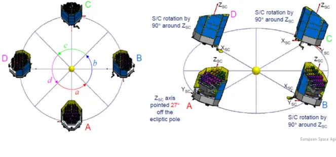
For example, during instrument calibration phases the satellite will be rotated by 90˝ around the payload line of sight to keep the solar panels and shields facing the Sun
(Figure 17). Also, images from the whole instrument field of view will be downlinked to the ground and used by the PMC to account for variations across the field of view such as the zodiacal light5. Furthermore, changes in the pointing direction of the instrument for switching between different LOP and SOP fields will also be performed during the calibration phases.
Figure 17 – Schematic of spacecraft rotation around payload line of sight to keep solar panels and shields facing the Sun.
Source: ESA.
2.8
Data products
All science data produced by the PLATO mission are categorized into three product levels that can be summarized6 as follows:
5 A detailed description of how to quantify the intensities of zodiacal light on PLATO cameras is provided
in subsection 3.1of this document.
• Level-0: comprises light curves, images and centroid curves of target stars from all individual telescopes, including eventual instrumental corrections applied on board only;
• Level-1: basically consists of Level-0 data that was calibrated and corrected for instrumental errors. These data will be mostly public available after calibration; • Level-2: comprises planetary candidates along with their respective transit depth,
transit duration, and estimated radius; list of planetary systems confirmed with TTVS, to be characterized by combining planetary transits and asteroseismology; results of asteroseismology analysis including stellar rotation periods, masses, radii and ages; and associated uncertainties;
• Level-3: list of confirmed planetary systems to be characterized by combining plane-tary transits, asteroseismology, and ground-based radial velocity follow-up.
2.9
Instrument description
2.9.1 Overall characteristics
The PLATO payload relies on an innovative multi-telescope concept consisting of
26 small aperture (12 cm pupil diameter) and wide circular field of view („1,037 deg2)
telescopes mounted in a single optical bench. Each telescope is composed of an optical unit (TOU), a focal plane assembly holding the detectors, and a front-end electronics (FEE) unit. The whole set is divided into 4 groups of 6 telescopes (herein called normal telescopes or N-CAM) dedicated to the core science and 1 group of 2 telescopes (herein called fast telescopes or F-CAM) used as fine guidance sensors by the attitude and orbit control system. The normal telescope assembly results in a overlapped field of view arrangement (see Figure 18), allowing them to cover a total sky extent of about 2,132 deg2, which represents almost 20 times the active field of the Kepler instrument. The N-CAM and F-CAM designs are essentially the same, except for their distinct readout cadence (25 and 2.5 seconds, respectively) and operating mode (full-frame and frame-transfer, respectively). In addition, each of the two F-CAM includes a bandpass filter (one bluish and the other
reddish) for measuring stellar flux in two distinct wavelength bands. Table 2 gives an
overview of the main payload characteristics based on (ESA, 2017).
2.9.2 Point Spread Function (PSF)
Starlight reaching the focal plane of PLATO cameras will inevitably suffer from distortions caused by both optics and detectors, causing this signal to be non-homogeneously spread out over several pixels. The physical model describing such effects is the PSF, from which one can determine – at subpixel level – how stellar signals are distributed over the
Figure 18 – Left: Schematic of one PLATO telescope. Centre: Representation of the PLATO spacecraft with 24+2 telescopes. Right: Layout of the resulting field of view obtained by grouping the normal telescopes into a 4 ˆ 6 overlapping configuration. The colour code indicates the number of telescopes covering the corresponding fractional areas (Table 2): 24 (white), 18 (red), 12 (green), and 6 (cyan).
Source: OHB-System AG (centre). The PLATO Mission Consortium (left and right).
Figure 19 – PLATO’s Teledyne-e2v 270 CCD.
Source: ESA.
pixels of the detector. This work uses synthetic optical PSF models obtained from the baseline telescope optical layout (Figure 20) simulated on ZEMAX R software. Estimated
assembly errors such as lens misalignment and focal plane defocus are included.
Beyond optics, the detectors also degrade the spatial resolution of stellar images through charge disturbances processes such as the charge transfer inefficiency (CTI) (Short et al.(2013), Massey et al.(2014)), “brighter-fatter” (Guyonnet et al.(2015)), and diffusion (Widenhorn(2010)). Several tests are being carried out by ESA to characterize such effects for the charge coupled devices (CCD) of PLATO cameras, so at the present date no formal specifications for the corresponding parameters are available. However, the optical PSFs alone are known to be a non-realistic final representation of the star signals. Therefore, to obtain a first order approximation of the real physics behind the PSF enlargement taking
Table 2 – Summary of main payload characteristics.
Description Value
Optics (24+2) telescopes
axisymmetric dioptric design
TOU Spectral range 500 ´ 1000 nm
Pupil diameter (per telescope) 12 cm
Detector back-illuminated
Teledyne-e2v CCD 270 (Figure 19)
N-CAM Focal Plane 4 full-frame CCDs
(4510 ˆ 4510 pixels each) F-CAM Focal Plane 4 frame-transfer CCDs
(4510 ˆ 2255 pixels each)
Pixel size 18 µm square
On-axis plate scale (pixel field of view) 15 arcsec Quantization noise „ 7.2 e´rms px´1
Readout noise (CCD+FEE) „ 50.2 e´rms px´1
Focal length 24.5 cm
Detector smearing noise „ 45 e´px´1s´1
Detector dark current noise „ 4.5 e´px´1s´1
N-CAM cadence 25 s
N-CAM exposure time 21 s
N-CAM readout time 4 s
F-CAM cadence 2.5 s
N-CAM field of view „ 1037 deg2 (circular)
F-CAM field of view „ 619 deg2
Full field of view „ 2132 deg2
Fractional field of view 294 deg2 (24 telescopes) 171 deg2 (18 telescopes) 796 deg2 (12 telescopes) 871 deg2(6 telescopes)
Source:ESA(2017).
place at PLATO detectors with respect to the diffusion, the optical PSFs are convolved to a Gaussian kernel with a standard deviation of 0.2 pixel. The resulting simulated PSF models are shown inFigure 21 for 15 angular positions, ξ, within the field of view of one camera. In this work, PSF shape variations due to target colour are assumed to be of second order and are thus ignored.
To reduce the overlap of multiple stellar signals and increase photometric precision, PLATO cameras are primarily designed to ensure that about 77% of the PSF flux is enclosed, on average, within „ 2.5 ˆ 2.5 pixels across the field of view, or 99% within