Arterial spin labeling performance in resting-state functional MRI: the effect of scan duration

HAL Id: tel-03139300

https://www.hal.inserm.fr/tel-03139300

HAL is a multi-disciplinary open access archive for the deposit and dissemination of sci-entific research documents, whether they are pub-lished or not. The documents may come from teaching and research institutions in France or abroad, or from public or private research centers.

L’archive ouverte pluridisciplinaire HAL, est destinée au dépôt et à la diffusion de documents scientifiques de niveau recherche, publiés ou non, émanant des établissements d’enseignement et de recherche français ou étrangers, des laboratoires publics ou privés.

Corentin Vallée

To cite this version:

Corentin Vallée. Arterial spin labeling performance in resting-state functional MRI: the effect of scan duration. Neuroscience. Université de rennes 1, 2020. English. �tel-03139300�

T

HÈSE DE DOCTORAT DE

L'UNIVERSITE

DE

RENNES

1

C

U

B

L

ECOLE DOCTORALE N°601

Mathématiques et Sciences et Technologies de l'Information et de la Communication Spécialité : Signal, Image, Vision

Arterial spin labeling performance in resting-state functional MRI: the

effect of scan duration

Thèse présentée et soutenue à Rennes, le 26/06/2020 Unité de recherche : IRISA

Par

Corentin Vallée

Rapporteurs avant soutenance :

Sophie Achard Directrice de recherche CNRS Laboratoire Jean Kuntzmann, Grenoble Patrícia Figueiredo Tenured Assistant Professor Instituto Superior Técnico, Lisboa

Composition du Jury :

Président : Michel Dojat Directeur de recherche Inserm Grenoble-Institut des Neurosciences, Grenoble Examinateurs : Sophie Achard Directrice de recherche CNRS Laboratoire Jean Kuntzmann, Grenoble

Patrícia Figueiredo Tenured Assistant Professor Instituto Superior Técnico, Lisboa Isabelle Corouge Ingénieure de recherche Université de Rennes 1, Rennes Dir. de thèse : Christian Barillot Directeur de recherche CNRS

Titre : Arterial spin labeling performance in resting-state functional MRI: the effect of scan duration

Mots clés : Arterial spin labeling, resting-state functional MRI, scan duration Résumé : L’arterial spin labeling en

resting-state (rsASL) dans la routine clinique et la recherche universitaire reste confidentiel par rapport à l'état de repos BOLD. Cependant, contrairement au BOLD, l'ASL permet un accès direct au flux sanguin cérébral (CBF), ce qui pourrait conduire à une application clinique importante à l'échelle du sujet, car l'ASL est une mesure non invasive du CBF (suivi des maladies avec déficience du CBF, études longitudinales de sujets sains, etc.). Malgré l'implication croissante de tous les acteurs de l'IRM dans l'ASL au cours de la dernière décennie, la question de la durée d'acquisition (DA) en rsASL semble n'avoir jamais été abordée dans la littérature, malgré ses fortes conséquences pratiques (mise en œuvre clinique et maintien de l’état de repos du sujet) et son impact sur la représentation des réseaux fonctionnels.

Dans cette thèse et comme travail préliminaire sur le sujet, nous discuterons tout d’abord de la manière d'étudier le rôle de la DA en rsASL avec des méthodes simples qui modélisent ce qu'un chercheur en rsMRI pourrait expérimenter. Nos résultats montrent que la représentation des réseaux fonctionnels se stabilise après une certaine durée d'acquisition pour des réseaux fonctionnels communs. Dans une deuxième partie, nous étudions les performance de l’ASL en resting-state par rapport au resting-state BOLD, tout en conservant la DA comme paramètre. Nous montrons que le rsBOLD surpasse la rsASL sur la plupart des aspects, mais pas sur tous. La possibilité de quantifier le CBF, contrairement au BOLD, tend à confirmer que le rsASL en particulier et l'ASL en général méritent encore plus d'implication de la part de la communauté de l’IRM fonctionnelle.

Title : Arterial spin labeling performance in resting-state functional MRI: the effect of scan duration

Keywords : Arterial spin labeling, resting-state functional MRI, scan duration Abstract :

(rsASL) in clinical routine and academic research remains confidential compared to resting-state BOLD. However, unlike BOLD, ASL provides with direct access to cerebral blood flow (CBF). This could lead to significant clinical subject scaled application as ASL is a non-invasive measurement of CBF (disease with CBF impairment follow-up, longitudinal studies of healthy subjects, etc.). Despite the significant increasing involvement of all MRI stakeholders is ASL over the past decade, the question of the acquisition duration (AD) in rsASL seems to have never been addressed in the literature, despite its strong practical consequences and its impact on functional networks representation.

In this thesis, and as a preliminary work on the subject, we will first discuss how to study the role of AD in rsASL with simple methods that model what a researcher in rsMRI might experience. Our results show that the representation of functional networks stabilizes after a certain acquisition time for common functional networks. In a second part, we study the performance of the ASL in resting-state compared to the BOLD resting-state, while keeping the AD as a parameter. We show that the rsBOLD outperforms the rsASL on most aspects, but not on all. The ability to quantify the CBF, unlike the BOLD, tends to confirm that rsASL in particular and ASL in general deserve even more involvement from the functional MRI community.

Acknowledgements

I would like to start by thanking Christian Barillot, Isabelle Corouge and Pierre Maurel for their supervision throughout this period. Their constant availability, support, and kindness have immensely helped me through the ups and downs of the PhD. I will always be thankful for sharing their experiences and advices with me during our animated meetings.

I would like to thank Sophie Achard and Patricia Figueiredo for reading the thesis and reporting on it with insightful remarks. I am also thankful to both of them and Michel Dojat for agreeing to be a part of the jury for the thesis defense. I would like to thank all the jury members again for providing their comments on this work.

I would like to thank Jean-Christophe Ferré and Michel Dojat for their wise feedback during PhD supervision committees.

I would like to thank Elise Bannier and the Neurinfo platform for the help in developing the MRI protocols, and thanks also to the subjects who participated in the study. I would like to thank Thomas Amand for his help in the organization of the visit in Beijing. I would like to express my special thanks of gratitude to Pr. Yu for making this visit possible, and his constant support during my stay.

I would also take this opportunity to thank Pr. Sui, Pr. Liu, Pr. Song, Pr. Jiang and their colleagues for their insightful opinions that have helped me identify the scopes for improving my work. Thanks also to Hua Jiaojiao, Han Xinyong, and Dai Rui for making my stay at Beijing a wonderful time.

I would now like to thank Pr. Klein, Pr. Caillau and Florian Brun without whose support motivated me to take up the PhD research.

Thanks also to the members of the Empenn team for making the work and the after-works so enjoyable.

I would finally like to extend a heartfelt thanks and gratitude to Christian Barillot. I would like to dedicate this manuscript to him.

ACKNOWLEDGEMENTS ... 1

CONTENTS ... 3

RESUME ... 7

INTRODUCTION ... 15

CHAPTER I.

CONTEXT ... 18

Section 1. Functional imaging ... 19

1.1 A brief history ... 19

1.2 Neurovascular coupling ... 20

1.3 Imaging techniques ... 23

Section 2. Functional magnetic resonance imaging ... 25

2.1 Introduction to Nuclear Magnetic Resonance ... 25

2.2 Functional MRI techniques ... 29

2.3 Application: task-based functional MRI ... 30

Section 3. Arterial Spin Labeling ... 31

3.1 General principle and declinations of ASL ... 31

3.2 CBF quantification ... 36

Section 4. Resting-state functional MRI ... 42

4.1 Introduction ... 42

4.2 Preprocessing resting-state fMRI data ... 44

4.3 Detecting functional networks with Seed-Based Analysis ... 47

4.4 Detecting functional networks with Independent Component Analysis ... 49

4.5 Alternative modeling methods ... 51

4.6 Organization of the resting-state networks... 52

4.7 Resting-state fMRI applications ... 54

4.8 Discussion ... 55

CHAPTER II.

THE EFFECT OF SCAN DURATION IN RESTING-STATE ASL ... 60

Section 5. Motivations ... 61 Section 6. Material ... 62 6.1 Subjects ... 62 6.2 MR Acquisition... 62 6.3 Data preprocessing ... 63 Section 7. Modeling ... 64

7.1 Detecting networks with Seed-Based Analysis ... 64

7.2 Evaluation scores ... 64

7.3 Modeling trend with respect to the duration... 67

Section 8. Results ... 68

8.1 How long is enough for the Default Mode Network? ... 68

8.2 How long is enough for all the networks? ... 72

Section 9. Discussion and conclusion ... 76

9.1 ASL feasibility ... 76

9.2 Acquisition duration ... 76

9.3 Methodological considerations ... 77

9.4 Conclusion ... 78

CHAPTER III.

STATE ASL PERFORMANCE COMPARED TO

RESTING-STATE BOLD

79

10.1 Motivation ... 80

10.2 Methodological consideration ... 80

Section 11. Comparing ASL and BOLD using MSDL references ... 82

11.1 Material and methods ... 82

11.2 Results for BOLD only ... 84

11.3 Comparison of ASL and BOLD ... 86

Section 12. Comparing ASL and BOLD without a reference ... 93

12.1 Foreword ... 93

12.3 Number of active voxels ... 94

12.4 Functional networks tissues distribution ... 97

12.5 Intrinsic functional connectivity of the functional networks ... 101

12.6 Spatial concordance between ASL and BOLD ... 105

12.7 Conclusion ... 109

CONCLUSION ... 110

APPENDIX ... 114

Resting-state ASL sequence parameters ... 115

Resting-state BOLD sequence parameters ... 117

Seeds Location in MNI152 coordinates ... 118

Boxplots of AUC distribution ... 119

LIST OF FIGURES ... 121

LIST OF TABLES... 123

LIST OF EQUATIONS ... 124

BIBLIOGRAPHY ... 125

Résumé

Dans cette section nous proposons un résumé en français du manuscrit. Nous conservons autant que possible la structure du document. Ce travail aborde l’effet de la durée d’acquisition sur les performances de l’arterial spin labeling (ASL) en imagerie par résonance magnétique (MRI) à l’état de repos. Le contexte de ce travail est présenté dans le premier chapitre du manuscrit. Le second chapitre est dédié à l’effet de la durée d’acquisition en resting-state ASL (rsASL), avec une attention toute particulière sur la méthodologie. Le troisième chapitre s’intéresse aux performances du rsASL par rapport à la technique actuelle de référence, le resting-state BOLD (Blood-Oxygen-Level-Dependent). Nous concluons dans le quatrième et dernier chapitre.

Introduction

En imagerie fonctionnelle, l’utilisation du resting-state ASL dans la routine clinique et pour la recherche académique reste limitée par rapport au resting-state BOLD. Cependant, contrairement au BOLD, l'ASL permet de quantifier la perfusion cérébrale. Cette caractéristique de l’ASL pourrait conduire à des applications cliniques importantes à l'échelle du sujet, car l'ASL est de fait une mesure non invasive du débit sanguin cérébral (DSC) : études longitudinales de sujets sains, suivi des maladies avec altération du DSC, etc. Malgré l'implication croissante de tous les acteurs de l'IRM dans l'ASL au cours de la dernière décennie, la question de la durée d'acquisition en rsASL semble n'avoir jamais été abordée dans la littérature, malgré ses fortes conséquences pratiques comme l’implémentation clinique, le maintien de l'état de repos par le sujet et, plus important encore, l'impact de la durée d'acquisition sur l’estimation des réseaux fonctionnels. Ce manuscrit à trois objectifs principaux. Le premier est de confirmer l'ASL en tant que technique viable pour l’IRM fonctionnelle à l'état de repos. Le deuxième est d'aborder l'effet de la durée d'acquisition sur l’estimation des réseaux fonctionnels. Le troisième est de tester les performances du resting-state ASL par rapport au resting-state BOLD, au regard de l’effet de la durée d’acquisition.

Chapitre I

La section 1 présente un bref contexte historique de l'étude des fonctions cérébrales qui a conduit au siècle dernier au développement rapide de technique d’imagerie fonctionnelle. Nous présentons également dans cette section le concept clé du couplage neurovasculaire. Le couplage neurovasculaire est l'interdépendance biologique qui existe entre l'activité électrique des neurones et le débit sanguin cérébral. Bien que le mécanisme exact du couplage neurovasculaire ne soit pas totalement élucidé, la réponse hémodynamique qui suit une activation neurale a été largement étudiée dans la littérature. Le principal avantage de cette connaissance de la réponse hémodynamique est que la fonction cérébrale peut être explorée non seulement par l'activation neuronale, mais aussi à partir des variations locales du débit sanguin cérébral. Nous terminons cette section en présentant des techniques d'imagerie qui, outre l'IRM, permettent d'étudier la fonction cérébrale, soit par l'activité électrique des neurones, ou bien par la réponse hémodynamique.

La section 2 présente un aperçu des bases de la résonance magnétique nucléaire (RMN). Comme l'IRM est notre technique d'imagerie fonctionnelle d'intérêt, nous présentons comment la RMN conduit à l'IRM. Nous introduisons également dans cette section les techniques d'IRM fonctionnelle, notamment l'IRM dynamique avec injection de produit de contraste (pour la mesure de perfusion cérébrale). Cependant, ce caractère invasif est discutable lorsque l'objectif est d'étudier une cohorte de sujets sains, ou encore dans le cadre d'une étude longitudinale.

La section 3 présente une dernière technique d'IRM fonctionnelle : l'imagerie de perfusion par marquage de spins du sang artériel, l’arterial spin labeling (ASL). Non invasive comme le BOLD, mais permettant la quantification du débit sanguin cérébral contrairement au BOLD, l'ASL est une technique d'IRM prometteuse qui malheureusement souffre d’une exposition limitée hors de la recherche académique.

Nous finissons par présenter avantages et limites de l'ASL en imagerie fonctionnelle, en particulier par rapport à la technique de référence qu’est le BOLD.

La section 4 présente l'IRM fonctionnelle au repos (rsfMRI). Au repos, le cerveau demeure actif : de nombreuses activations spontanées des neurones se produisent. La connectivité fonctionnelle est définie comme la concomitance de ces activations neuronales spontanées. Les zones dédiées à la même fonction montrent une forte connectivité fonctionnelle, comme l'a illustré la toute première expérience d'IRM fonctionnelle à l’état de repos avec l'aire motrice. L'étude de la connectivité fonctionnelle permet de subdiviser le cerveau en petites unités fonctionnellement cohérentes, appelées réseaux fonctionnels, et de montrer comment leur architecture globale a la propriété de graphe petit-monde chez le sujet sain. Dans cette section, nous définissons tout d'abord la connectivité fonctionnelle et présentons l’IRM de repos. Dans un second temps, nous présentons le prétraitement des données de rsfMRI ainsi que différents modèles de connectivité fonctionnelle qui permettent la reconstruction de réseaux fonctionnels. Enfin, nous introduisons brièvement la théorie des graphes, qui est un outil particulièrement adapté à la compréhension de l'organisation fonctionnelle du cerveau. Au-delà de la compréhension des fonctions cérébrales, l'IRMf au repos trouve également des applications cliniques. En effet, la neuropathologie peut affecter la disposition des réseaux fonctionnels et défaire l’organisation petit-monde des réseaux, à l'échelle du graphe. La section consacrée à l’IRM de repos se termine par une discussion qui guidera notre modélisation dans la partie suivante du manuscrit et permettra également de commenter les résultats obtenus.

Chapitre II

La section 5 motive nos premières contributions. La durée d'acquisition est un paramètre pratique essentiel dans une étude rsfMRI. Quelques articles ont déjà étudié directement ou indirectement l'influence de la durée en resting-state BOLD [Anderson et al., 2011; Birn et al., 2013; Bouix et al., 2017; Laumann et al., 2015; Termenon et al., 2016; Van Dijk et al., 2010]. Cependant, à notre connaissance, la question n'a pas encore été abordée en rsASL. Dans la deuxième partie de ce manuscrit, nous abordons donc l'influence de la durée d'acquisition en resting-state ASL. Afin de confirmer la viabilité de l'ASL comme technique d’IRM au repos, nous insistons également sur la faisabilité de la détection des réseaux fonctionnels cérébraux avec l’ASL. La plupart des études actuelles sur le resting-state ASL proposent une durée de 8 à 13 minutes et un TR de 3 à 4 s (soit 120 à 260 volumes). Intuitivement, on pourrait supposer que plus la durée est longue, plus l'échantillonnage de la corrélation des signaux (ou de toute autre mesure sur les signaux) dans le cerveau est bon et donc meilleure est l'acquisition. Toutefois, cela nécessite de définir ce que signifie réellement une "meilleure" acquisition, et cela ne tient pas compte des conditions cliniques et de maintien de l’état de repos du sujet.

La section 6 présente les paramètres d’acquisitions et le prétraitement des données utilisé. Nous nous efforçons de rester aussi proches que possible de ce qu'un chercheur en resting-state ASL pourrait classiquement expérimenter, en mettant en œuvre une séquence ASL habituelle et un prétraitement des données typique. Comme nous voulons

confirmer la faisabilité de l'ASL en tant que technique de rsfMRI, nous nous concentrons sur une étude à l'échelle du sujet.

La section 7 décrit les méthodes utilisées pour détecter les réseaux fonctionnels et modéliser leur évolution en fonction de la durée d’acquisition. Pour la modélisation de la connectivité fonctionnelle, nous nous appuyons sur une analyse de type « seed-based analysis » (SBA) qui facilite la comparaison directe entre les sujets. Afin d'évaluer l'effet de la durée d'acquisition sur la qualité des réseaux détectés par resting-state ASL, nous imitons le comportement d'une inspection visuelle des données. Un investigateur confirmerait qu'un réseau estimé est valide si l'estimation est proche d'une définition consensuelle du réseau attendu. Nous modélisons l'énoncé "proche d'une définition consensuelle" en associant un score au recouvrement entre un réseau fonctionnel estimé et un réseau de référence correspondant, provenant d'un atlas de rsfMRI, l'atlas Multi-Subject Dictionary Learning (MSDL) [Varoquaux et al., 2011]. Nous utilisons la régression locale LOESS pour modéliser l’évolution des scores en fonction de la durée d’acquisition. La section 8 est axée sur les résultats. Une analyse approfondie du réseau du mode par défaut (DMN) est présentée afin d'illustrer l'évolution des scores sur le réseau le plus typique de la rsfMRI. Pour tous les sujets, l'indice de Jaccard et l'aire sous la courbe (AUC) se stabilisent après une durée d'acquisition similaire, en adéquation avec l'interprétation de l'inspection visuelle. Comme tous les réseaux fonctionnels sont détectés à l'échelle du sujet, nos résultats confirment la faisabilité de L’ASL comme technique de resting-state MRI. En outre, nos résultats montrent une stabilisation de la qualité de l’estimation après un certain nombre de volumes/une certaine durée pour chaque réseau fonctionnel d'intérêt.

La section 9 discute les résultats et conclut ce chapitre du manuscrit. Comme la qualité des réseaux fonctionnels se stabilise après une certaine durée pour toutes les graines (seeds), la durée optimale peut donc être définie par le début de la stabilisation, interprétée comme un compromis entre la mise en œuvre clinique (la durée la plus courte possible) et les meilleures estimations de réseaux (couverte par des durées très longues). En suivant cette proposition, nous pouvons suggérer, pour notre ensemble de paramètres d’acquisition et de prétraitement, un nombre optimal de volumes de 240, correspondant à une durée optimale de 14 min. Comme nous avons utilisé un prétraitement basique, toute méthode qui améliore la détection des réseaux fonctionnels est susceptible de fournir un début de stabilisation plus précoce, c'est-à-dire un nombre de volumes plus faible et une durée optimale plus courte. Notre suggestion de 240 volumes devrait ainsi suffire pour fournir la meilleure estimation possible des réseaux pour la plupart des utilisations de resting-state ASL.

Chapitre III

La section 10 introduit la comparaison entre le resting-state ASL et le resting-state BOLD. Nous soulignons dans cette section quelques considérations méthodologiques avant de passer à la comparaison. Bien que distinctes dans l’approche, les deux techniques d’IRM mesurent indirectement une activation neurale, et ainsi les prétraitements sont presque interchangeables entre les deux modalités. Cependant, en ce qui concerne l’effet de la durée d'acquisition, la question est plus subtile. En effet, comme le signal est traité

numériquement, on ne peut pas simplement faire la comparaison par rapport à une durée : le nombre d’éléments de l'échantillon utilisé pour estimer une carte fonctionnelle n'est pas une durée en minutes, mais correspond en fait au nombre de volumes. Ainsi, en comparant les cartes fonctionnelles par rapport au nombre de volumes, si une carte est meilleure qu'une autre, ce n'est pas parce qu'elle a été estimée avec une taille d'échantillon plus importante.

La section 11 détaille la comparaison entre ASL et BOLD en appliquant tout d’abord aux données state BOLD le cadre d’évaluation que nous avons utilisé pour le resting-state ASL. Première étape, le prétraitement : il est commun entre le resting-resting-state BOLD et le resting-state ASL, mis à part l’étape de soustraction inter-volume propre à l’ASL. Deuxièmement, la seed-based analysis est également directement applicable : nous utilisons les mêmes graines. Troisièmement, la modélisation et les scores ne dépendent pas de la technique d’acquisition utilisée. Par conséquent, dans cette section, les données rsBOLD sont analysées en suivant la même méthodologie que celle proposée pour les données ASL, puis les résultats sont comparés à ceux obtenus en rsASL dans la partie précédente. Dans l'ensemble, la détection des réseaux semble plus facile en BOLD car plus de graines parviennent à fournir des estimations satisfaisantes des réseaux fonctionnels. Les deux scores de recouvrement par rapport aux références MSDL (indice de Jaccard et AUC) sont légèrement meilleurs en BOLD qu'en ASL. Une stabilisation peut également être observée en BOLD. Cependant, la variance intra-sujet et inter-sujets est beaucoup plus importante en BOLD qu'en ASL : les courbes de régression LOESS sont moins corrélées entre les sujets mais surtout moins corrélées entre les scores. Par conséquent, il est plus difficile en BOLD de définir avec précision un début de stabilisation car l’AUC suggère clairement un nombre plus élevé de volumes, quelle que soit la définition de la stabilisation considérée. Si l'on utilise les mêmes considérations qu'en ASL, c’est-à-dire un compromis entre la durée la plus courte possible pour l’implémentation clinique et la plus longue pour garantir avec le plus de certitude possible la stabilisation, la fourchette de valeurs optimales se situe pour le BOLD entre 250 et 290 volumes (contre 240 en ASL).

La section 12 présente des méthodes alternatives pour comparer l’ASL et le BOLD en resting-state, toujours en fonction du nombre de volumes. En effet, dans la section précédente, la comparaison est effectuée par le biais d'un atlas tiers : le MSDL. En étudiant une technique seule, l'impact de l'utilisation d'un atlas est limité, car il a un impact sur la hauteur des scores, mais pas sur le phénomène de stabilisation. Cependant, comme le MSDL dérive de données BOLD, le BOLD est très probablement avantagé. Dans cette section, nous comparons directement les cartes fonctionnelles obtenues par resting-state ASL et resting-state BOLD à travers quatre mesures. Tout d'abord, nous présentons le nombre de voxels actifs. Il s'agit simplement d'une mesure de la taille des réseaux fonctionnels correspondants. Nous montrons que quel que soit le nombre de volumes, les réseaux fonctionnels BOLD sont toujours 2 à 3 fois plus grands que les réseaux fonctionnels ASL correspondants. Ensuite, nous étudions la distribution tissulaire des réseaux fonctionnels estimés. En effet, nos réseaux fonctionnels d'intérêt devraient avoir la plupart de leurs voxels situés dans la matière grise, un peu dans la matière blanche, et aucun dans le liquide céphalorachidien. Malgré la grande différence de taille,

la distribution tissulaire des réseaux fonctionnels estimés est en fait extrêmement homogène entre l'ASL et le BOLD. Peu importe la graine, le sujet, le nombre de volumes, la technique IRM, la distribution tissulaire est pour presque chaque réseau estimé comme suit : 55-60% dans la matière grise, 25-30% dans la matière blanche, 10-15% dans le liquide céphalorachidien. En d'autres termes, étant donné une distribution tissulaire, il n'est pas possible de prédire à quelle technique d’acquisition elle correspond : la distribution tissulaire n'a pas de pouvoir discriminant. Troisièmement, nous étudions la connectivité fonctionnelle intrinsèque des réseaux fonctionnels estimés. Interprétée comme le résultat d’une classification statistique (clustering), on souhaite qu’une estimation d'un réseau fonctionnel, c'est-à-dire d'un cluster, ait une variance intra minimale, c'est-à-dire une connectivité fonctionnelle intrinsèque maximale. Nous montrons que peu importe les graines, les réseaux fonctionnels estimés avec succès ont une bien meilleure connectivité fonctionnelle intrinsèque en rsASL qu'en rsBOLD. Nous terminons la section en étudiant la corrélation spatiale entre l'estimation en rsASL et en rsBOLD. En ce qui concerne le nombre de voxels actifs, nous utilisons les informations préalables pour ne considérer que les graines qui sont capables de détecter efficacement un réseau fonctionnel. Pour chaque graine, la corrélation spatiale se comporte comme la LOESS lui correspondant dans la modélisation précédente : un faible nombre de volumes est associé à une faible corrélation spatiale, et il est intéressant de noter qu'après un nombre de volumes proche de la fourchette où nous avons détecté la stabilité avec le MSDL, la corrélation spatiale entre les cartes fonctionnelles rsASL et rsBOLD atteint ses valeurs les plus élevées et reste stable avec un plus grand nombre de volumes. Cela confirme que l'impact de l'utilisation d'un atlas est extrêmement limité dans l'apparition du phénomène de stabilisation. En effet, on aurait pu objecter que l'estimation des réseaux fonctionnels peut osciller autour de sa référence, et qu'une stabilisation du score ne traduit pas totalement une stabilisation de la disposition spatiale. Cependant, le cas où une estimation de réseau fonctionnel oscille autour d'une référence MSDL par rapport à l'indice de Jaccard, et oscille également autour de la référence par rapport à la AUC est déjà très difficilement réalisable. Avec ces informations auxiliaires, la stabilisation de la corrélation spatiale confirme la stabilisation de l'agencement spatial des réseaux fonctionels en rsASL et en rsBOLD après une certaine durée.

Chapitre IV

La dernière partie du manuscrit synthétise les résultats du travail effectué au cours de cette thèse et propose quelques perspectives. Dans ce manuscrit, nous nous sommes concentrés principalement sur les considérations méthodologiques de cette évaluation. L'IRM fonctionnelle étant un champ de recherche extrêmement vaste, les facteurs qui pourraient affecter le nombre optimal de volumes à utiliser sont nombreux. Heureusement, beaucoup de ces paramètres disposent de leur propre littérature. De plus, nous avons essayé de mettre en place des séquences et des traitements suffisamment généraux de tel sorte que le nombre de volumes que nous proposons couvre presque tous les usages de la rsASL. Les séquences et traitements appliqués sont aussi suffisamment standards afin de montrer que la rsASL est parfaitement viable en tant que technique de rsfMRI. À notre avis, une meilleure compréhension de l’effet de la durée d’acquisition est à chercher du côté de deux paramètres de la séquence : le temps de

répétition (TR) et le délai post-marquage (PLD). Nous souhaiterions en effet fournir une durée optimale d’acquisition en rsASL en minutes, et non en nombre de volumes, notamment pour la mise en œuvre clinique. Comme le temps de répétition lie les deux, il semble que son rôle spécifique soit le sujet naturel de recherche à approfondir. Le PLD peut également jouer un rôle décisif : un PLD plus long favorise une meilleure estimation du débit sanguin cérébral tandis qu'un PLD plus court favorise une meilleure estimation des réseaux fonctionnels. Comme il n'y a pas de meilleure option à choisir entre les deux, nous avons conservé un PLD long car le principal avantage de l'ASL par rapport au BOLD, est la possibilité de quantifier le débit sanguin cérébral. Par conséquent, l’effet du PLD sur le phénomène de stabilisation des réseaux fonctionnels semble extrêmement intéressant à étudier pour le resting-state ASL.

Introduction

Understanding the brain function has been an important area of research for millennia. The recent fast development of neuroscience in the last century, and in particular the emergence of neuroimaging techniques, has opened the field for in vivo investigations of the cerebral activity. In particular, Functional Magnetic Resonance Imaging (fMRI), thanks to its non-invasiveness and good spatial resolution, has been widely used to assess brain function, through two techniques: task-based fMRI and resting-state fMRI. Task-based fMRI confronts the subject to particular stimuli, which are expected to activate a corresponding specific functional area. In resting-state fMRI (rsfMRI), the subject does not perform any task nor is confronted to any stimuli. However, the similarities in the pattern of spontaneous neural activations at rest provide valuable information on brain function and define the functional connectivity of the brain. Indeed, brain regions can be structurally remote yet have strong a strong functional connectivity, forming what is called a functional network. RsfMRI provides a better understanding of the brain function and especially the organization of the brain into functional networks. RsfMRI has also found numerous clinical applications, as healthy subjects and patients show differences in functional connectivity, in common pathologies like Alzheimer’s disease, multiple sclerosis and schizophrenia.

In resting-state functional MRI the gold-standard technique is the Blood-Oxygen-Level-Dependent (BOLD) fMRI. However, due to the multifactorial nature of the BOLD signal, its measure of neural activation is indirect and relative. Arterial Spin Labeling (ASL) is an MRI technique which uses magnetically labeled arterial water protons as an endogenous tracer. An inversion pulse labels the inflowing blood and after a delay called post-labeling delay, a labeled image of the volume of interest is acquired. The subtraction of the labeled image from a control image, i.e., non-labeled, reflects the quantity of spins that have perfused the imaged volume, producing what is commonly called a perfusion-weighted (PW) image. The brain perfusion is the biological process that insures the delivery of oxygen and nutrients to the cerebral tissues by means of microcirculation. The

PW map can be used to quantify the cerebral blood flow (CBF) under some assumptions. The quantification of CBF is the main advantage of ASL over BOLD. The absence of injection and the possibility to employ this imaging technique to brain function or basal perfusion is very attractive. This could lead to significant clinical subject scaled application as ASL is a non-invasive measurement of CBF. Even though the principle of ASL were introduced around the same time of BOLD fMRI, resting-state ASL (rsASL) research has a limited exposure in clinical routine and academic research compared to resting-state BOLD (rsBOLD). The main explanation is probably the lower signal-to-noise ratio of ASL compare to BOLD and its harder practical implementation. Despite the increasing involvement of all MRI stakeholders in ASL over the past decade, much still needs to be done to provide standardized implementation and processing. In particular, the question of the acquisition duration in rsASL seems to have never been addressed in the literature despite its strong practical consequences: clinical implementation, resting-state upholding by the subject, and more importantly, the impact of acquisition duration on the estimation of functional networks.

This manuscript has three main objectives. The first one is to confirm ASL as a viable resting-state fMRI technique. The second one is to address the effect of scan duration on the functional networks estimation. The third one is to test rsASL performance against rsBOLD with respect to the scan duration.

Plan

Chapter I – Context

Section 1 presents an historical background of investigation of the brain functions that led in the last century to the rapid development of functional imaging. We also present in this section the key concept of the neurovascular coupling and the imaging techniques that, besides MRI, allow the investigation of brain function.

Section 2 presents an overview of the basics in nuclear magnetic resonance (NMR) and how NMR leads to MRI. We also introduce in this section functional MRI techniques, particularly the gold-standard of functional MRI technique: the blood-oxygen-level dependent (BOLD) functional MRI.

Section 3 presents the technique of interest of this manuscript: arterial spin labeling (ASL). Non-invasive as BOLD, but allowing the computation of CBF unlike BOLD, ASL is a promising MRI technique for clinical application.

Section 4 reviews the resting-state functional MRI (rsfMRI). We first define functional connectivity and present preprocessing of rsfMRI data, different modeling of the functional connectivity that allow the reconstruction of functional networks, and lastly, we briefly introduce the graph theory that provides practical insight into the understanding of brain functional organization. This rsfMRI section ends with a discussion of the definitions and methods, that guides our modeling in the following parts of the manuscript and also help to discuss the results afterwards.

Chapter II – The effect of scan duration in resting-state ASL

Section 5 motivates our first contributions on the effect of scan duration in resting-state ASL (rsASL) and the feasibility of rsASL.

Section 6 presents material and preprocessing used in the second chapter of the manuscript. We remain as close as what a typical investigator of rsASL might experience, by implementing a usual ASL sequence and typical rsfMRI preprocessing and focusing on a subject-scaled study, as estimating network on a subject is harder than on a group.

Section 7 describes the methods. For the modeling of functional connectivity, we rely on seed-based analysis (SBA). In order to assess a trend in the duration influence on rsASL detected networks quality, we score the overlap between an estimated functional network and a corresponding reference network from an atlas of rsfMRI.

Section 8 focuses on results. After describing the scores used and the modeling of their evolution over time using a LOESS, an in-depth analysis for the Default-Mode Network (DMN) is presented in order to illustrate scores evolution on the most typical resting-state network. For all subjects, scores stabilize after a similar scan duration, in adequation with visual inspection. Finally, we show results for five additional typical functional networks. As all functional networks are detected at a subject scale, our results confirm the feasibility of rsASL. Furthermore, our results show a stabilization after a certain number of volume/duration for every functional network of interest.

Section 9 discusses the results and concludes this part of the manuscript. We suggest 240 volumes / 14 min for rsASL as a sufficient amount of data to obtain stabilized and best estimation of functional networks.

Chapter III – Resting-state ASL performance compared to resting-state BOLD

Section 10 introduces the comparison between rsASL and rsBOLD. As rsBOLD technique is the gold-standard for rsfMRI, the performance of rsASL should be compared to rsBOLD. We point out in this section some methodological considerations in the comparison.

Section 11 details the comparison using the methodological framework we used for rsASL. Overall, the detection of networks seems easier in BOLD. Overlap scores are slightly better in BOLD than in ASL. A stabilization stage can also be observed with BOLD. If we use the same considerations as in rsASL that lead to suggest 240 volumes, the range of suggested values for BOLD is between 250 and 290 volumes.

Section 12 presents alternative methods for comparing rsASL and rsBOLD with respect to the number of volumes. In the previous section, the comparison is actually made through a third-party atlas. In this section, we directly compare rsASL and rsBOLD functional maps through four different measures: the number of active voxels, the tissue distribution, the intrinsic functional connectivity and the spatial correlation.

Conclusion

The last part of the manuscript gathers the results of the work done in the manuscript and suggest area for future investigation.

Chapter I.

Context

Section 1.

Functional imaging

In this section we introduced an historical background of investigation of the brain functions and the concept of neurovascular coupling that leads in the last century to the rapid development of functional imaging.

1.1

A brief history

Brain depictions could already be found in ancient Egypt, as Figure 1.1 illustrates. Since that age, the brain anatomy secrets have been continuously discovered with the increasing accuracy of tools, procedures and also accuracy of investigators. However, brain functions in the human body have resist the physicians for several millennia. Before the recent fast development of neuroscience in the last century, brain functions were unfortunately discovered through trauma, like aphasia resulting from a head injury already reported in Egyptians papyrus. While eminent thinkers like Aristotle conceived the brain as a blood cooling mechanism, the antic philosopher Alcmeon of Croton (5th

century B.C.) made the first ever reported true assumption about brain functions: “The seat of sensations is in the brain. This contains the governing faculty. All the senses are connected in some way with the brain; consequently, they are incapable of action if the brain is disturbed” [Gross, 1987]. In order to find a first evidence of Alcmeon hypothesis, we need to wait more than two millennia before Legallois’s experiment in 1811. A few years after the discovery of the role of electricity in the nervous system, Legallois’s point was to show that a tiny lesion in a specific area in the brain could totally block the respiratory system [Bruce Fye, 1995]. Legallois corollary showed for the first time that a specific cerebral area is used in a specific physiological function. In the end of the same

Figure 1.1: The Edwin Smith surgical papyrus (-1700 B.C.) and a partial translation The partial translation comes from [Breasted, 1930]. As Breasted state, the hieroglyphs evoke “organic substance of a viscous or semifluid consistency”. While enigmatic alone, its rare occurrences are most often followed by “of his skull”, giving no doubt on his meaning. This is the eldest designation of the brain in mankind history.

century, in 1881, a capital experiment was made by Mosso, who managed to exhibit a link between a cognitive task and variations in blood-flow [Raichle and Shepherd, 2014]. These historical elements give main objectives of functional imaging: measuring cerebral activity, associating areas of the brain with physiological roles, called functions, investigating how these areas interact, through the measurement of the electric activity of the brain or the cerebral blood supply. By extension, functional imaging is also about investigating numerous pathologies since alterations in the brain energy supply or electrical activity can lead to physiological impairment.

1.2

Neurovascular coupling

In the early 20th _{century, the rapid development of tools to investigate microanatomy}

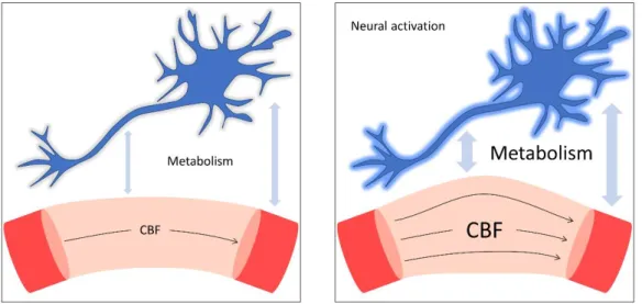
(histology), biochemistry and microbiology led to a better understanding of the brain energy supply through blood. However, as soon as in 1890, Roy and Sherrington described a key principle of functional imaging: the neurovascular coupling [Roy and Sherrington, 1890]. Neurovascular coupling is the biological interdependence that exists between the neurons electrical activity and the cerebral blood flow (CBF). Figure 1.2 illustrates this relationship. While the relationship between neural activation, local metabolism and CBF increase is factual, the exact underlying mechanism behind the coupling is still an active field of research [Huneau et al., 2015]. Numerous functional imaging techniques benefit from this coupling. Indeed, they can hence infer variations in cerebral activity not only through neuron electrical activity, but also through the investigation of the cerebral hemodynamic variations.

Figure 1.2: Neural activation and neurovascular coupling

When confronted to a stimulation, a neuron releases an electrical signal. The electro-chemical activity of the neurons increases the local metabolism. Since the metabolism is fueled by the blood of the surrounding capillaries, the neuron activation also requires a local increase of the cerebral blood flow.

1.2.1 Hemodynamic response

The hemodynamic response function (HRF) represents the expected variation in cerebral blood flow (CBF) as a function of time following a neuronal activation. This standard (canonical) model admits a high variability according to individuals, spots/stimuli and sequences, see [Aguirre et al., 1998; Silvestre et al., 2010] for advanced modeling of the HRF. Figure 1.3 shows a generic model of the hemodynamic response. The initial dip detected by Buxton [Buxton, 2001], that occurs within the first two seconds after the stimulus is generally ignored in models [Poldrack et al., 2011]. Its negative intensity is low compared to the maximum hemodynamic response, so it is rarely observed in practice.

Figure 1.3: Canonical shape of the hemodynamic response function

Abscissa unit is arbitrary. After a neural activation, it takes approximatively twenty seconds before the comeback of the basal state.

1.2.2 Linear time invariant property

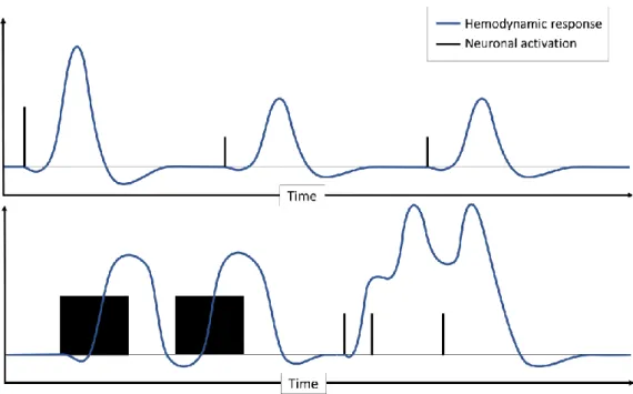
An important assumed property of the hemodynamic response is its linear relationship with the neural activation. This assumption is called the linear time invariant (LTI), and greatly simplifies the modeling and interpretation of neuroimaging investigation. Overall, the LTI assumption appears to be fairly accurate in most cases [Dale and Buckner, 1997; Logothetis et al., 2001]. It shows some limitations when the subject is stressed by the stimuli, i.e. when stimuli frequency becomes too high [Wager et al., 2005]. In this case, neural responses can saturate, while the cerebral blood flow keeps increasing [Sheth et al., 2004]. On the opposite, too short and/or too small neural activations are not associated with a CBF increase [Sheth et al., 2004]. The stimuli type can also thwart the linearity, like auditive stimuli [Harms and Melcher, 2002]. Nonetheless, the range of investigations where the LTI is satisfied is wide. Figure 1.4 illustrates the LTI property.

Figure 1.4: Illustration of the linear time invariant property of the HRF

The top graph shows how the HRF amplitude depends linearly on the neuron activation intensity: halving the activation intensity also halves the hemodynamic response, and two identic activations produced two identic responses (from basal state). The bottom graph shows more sophisticated neuronal activations and their associated responses. Since we assume the linearity, the expected HRF is simply the convolution between the canonical HRF and the function that describe the neural activation with respect to time. This computation is the core of task-based functional MRI, which is addressed in section 2.3.

1.3

Imaging techniques

In this section, we briefly describe some common functional imaging techniques. Thanks to the neurovascular coupling, these techniques can measure directly or indirectly either the electrical activity of the neurons or associated hemodynamic response parameters. 1.3.1 Electroencephalography (EEG)

The communication between the brain neurons is made through synapses with electro-chemical reactions. One of the most natural way to investigate brain activity is to measure this electrical activity. EEG uses electrodes placed on the patient scalp to record the variation in voltage between these electrodes resulting from the chemical reaction between synapses [Henry, 2006]. Compared to other brain imaging techniques, EEG is one of the cheapest, easiest to implement and less invasive methods (apart from its intracranial counterpart), which perfectly suits the study of large cohort of healthy (or not) subjects. Furthermore, EEG has one of the best temporal resolution with the order of the millisecond. The major EEG downside is its poor spatial resolution which does not allow an accurate localization of the brain functional activity. However, the increasing development of multimodal brain imaging allows to use EEG in combination with a more spatially accurate method, typically MRI, to overcome EEG poor spatial source localization [Abreu et al., 2018; Bießmann et al., 2011]

1.3.2 Magnetoencephalography (MEG)

Magnetoencephalography is the magnetic equivalent of the EEG: instead of recording voltages, it uses magnetometers to record the magnetic field induced by the brain electric activity [Hämäläinen et al., 1993]. MEG and EEG are similar regarding their imaging properties. MEG is can also be used in combination with other brain imaging technique, and often with EEG as recording both at the same time is quite straightforward [Lopes da Silva, 2013].

1.3.3 Near-infrared spectroscopy (NIRS)

Widely use in chemistry to identify organic molecules, NIRS assess brain activity by recording optical transmittance variation caused by the variation in blood hemoglobin concentration, in the near-infrared spectrum. Indeed, a neural activation requires energy which is drawn from the oxygen stored in the blood hemoglobin, locally modifying its concentration [Butler et al., 2017]. As EEG, NIRS is cheap and non-invasive. However, NIRS records indirectly the brain activity and only through the cortical surface, which hinders its interpretation.

1.3.4 Positron emission tomography (PET)

We briefly mentioned in the NIRS section that a neural activation requires chemical energy, which is brought to the neurons through the vascular system. Hence, tracing this chemical supply would provide direct exhibition of the neural activity, which is the exact concept of PET. PET consists in injecting a radioactive component, like 15O (called radiotracer), and investigating its spreading and accumulation in the brain by tracing its radioactivity with a gamma camera [Vaquero and Kinahan, 2015]. The major advantage of PET is that it allows to quantify the cerebral blood flow, depending on the radiotracer

used. As neural activity is directly related to the oxygen consumption, and oxygen consumption to cerebral blood flow (cf. neurovascular coupling in section 1.2), PET scan allows a quantitative measurement of the neural activity as well as the investigation of disease that have an impairment of cerebral blood flow as biomarker, such as Alzheimer’s disease [Marcus et al., 2014]. PET major limitation is the injection of radioactive components, which usage is arguable when investigating healthy subjects.

1.3.5 Computed tomography (CT)

The CT cast series of X-rays on the subject in different direction. Since each organic component has its own level of X-ray absorption, and also because the body absorption is not high enough to totally cancel the penetrating ability of X-rays, CT is able to rebuild the head as a three-dimensional volume and also differentiating tissues inside it [Ter-Pogossian, 1984]. In order to quantify perfusion, an intravenous contrast agent with known pharmacokinetic is injected to the subjects. The high contrast of CT, its faster and less constraining implementation compared to MRI, has made the technique of choice in emergency case and for pathologies related to head trauma However, CT has a major downside. The X-rays are energetic enough to interfere with molecular structure, and are prone to increase the risk of cancer. Consequently, CT is not suitable for longitudinal studies, especially for research purpose on healthy subjects where the benefits of examination are highly arguable.

Note that even though computed tomography usually refers to specifically X-rays, tomography is actually every technique that (re-)build a three-dimensional volume from a sample of two-dimensional sections. For instance, MRI can somehow be understood as a nuclear magnetic resonance tomography. Functional MRI is detailed in next chapter.

Section 2.

Functional magnetic resonance imaging

The phenomenon of nuclear magnetic resonance has been discovered simultaneously in 1946 by the respective teams of F. Bloch's in Stanford and E. Purcell at Harvard, and both were awarded the Nobel Prize in 1952. Currently, the phenomenon is mainly known for its use in the medical field as magnetic resonance imaging (MRI). Beside the detection of structural brain abnormalities such as tumors or lesions, the MRI saw in the 1990s the development of a new application, so-called functional MRI (fMRI).

2.1

Introduction to Nuclear Magnetic Resonance

This section overviews the basic principle of nuclear magnetic resonance imaging (NMR) that allows imaging to be made.

2.1.1 Quantum model

The human body consists of roughly two third of hydrogen atoms H1 . In NMR, we usually assimilate the proton H1 + with the hydrogen atom. A proton is a positively charged elementary particle that rotates on itself along a free axis, whose guiding vector 𝑆⃗ represents the spin of the particle.

Let us give a strong magnetic field B⃗⃗⃗0 of the order of several Tesla: 0.5T to 22T in general,

less than 11.5T for the medical environment (4.10-5_{T for the earth magnetic field as a}

comparison). Let this field be oriented according to Oz, in the canonical coordinate system of ℝ3, without any loss of generality. The protons spins evolving in this magnetic field will align on B⃗⃗⃗0, either in parallel or in antiparallel direction. The quantum mechanics

guarantees that there will always be slightly more protons in the same direction as B⃗⃗⃗0,

around two parts-per-million in standard condition for temperature and pressure for 0.5T field. This may seem like a small amount, but as a reminder, one gram of hydrogen (i.e. one gram of proton) represents one mole of hydrogen, i.e. 6.02×1023 _{atoms. This}

difference of "excess" protons induces a macroscopic magnetization of the protons represented by a vector M⃗⃗⃗⃗ = M⃗⃗⃗⃗z₀ along the Oz axis. For a family of N protons indexed by

𝑖 we have: • Without B⃗⃗⃗0 : ∑N𝑖=1S⃗⃗𝑖 = 0⃗⃗ • Under B⃗⃗⃗0 : (∀𝑖 ≤ N, S⃗⃗𝑖 = ±S⃗⃗) ∶ ∑𝑁𝑖=1S⃗⃗𝑖 ≅ N 2. S⃗⃗ − N 2. S⃗⃗ + 2. 10 −6_{. N. S⃗⃗ = M⃗⃗⃗⃗} z0 2.1.2 Electromagnetic pulse Precession

So far, we have considered the protons spins as perfectly aligned with the field B⃗⃗⃗0. In fact,

this is not exactly true, the axis carried by every spin S⃗⃗𝑖 rotates around B⃗⃗⃗0 at a fixed angle

with a frequency 𝜔0. This phenomenon is called the precession. This is exactly the exact

same phenomenon that can be observed when disturbing the rotation of a spinning top. The proton revolves around S⃗⃗𝑖 and S⃗⃗𝑖 revolves around B⃗⃗⃗0.

Resonance

A new field B⃗⃗1 , orthogonal to B⃗⃗⃗0 and called a radio-frequency pulse (RF), is applied. It

this context Larmor frequency, the field B⃗⃗⃗1 resonates with the precession of the protons.

This field will force the protons to orient themselves in antiparallel with B⃗⃗⃗0. The protons

perform this movement with the same phase, which will gradually make the longitudinal component M⃗⃗⃗⃗z disappear in favour of a transverse component M⃗⃗⃗⃗xy. When half of the

"excess" protons have turned around, the longitudinal component has disappeared, and ‖M⃗⃗⃗⃗xy‖ is maximum (90° RF Pulse). If the RF wave continues to be applied, all the spins in

excess are turned around, ‖M⃗⃗⃗⃗xy‖ = 0 and M⃗⃗⃗⃗z= −M⃗⃗⃗⃗z₀ (180° RF pulse).

Relaxation

The state of the protons spin caused by the field B⃗⃗⃗1 is unstable, hence when the RF pulse

stops, the protons tend to return to the initial state, without a transverse component ‖M⃗⃗⃗⃗xy‖ and with: M⃗⃗⃗⃗ = M⃗⃗⃗⃗z= M⃗⃗⃗⃗z0. For an RF pulse of 90°, two characteristic times will

interest us:

• T1 characterizing the longitudinal relaxation, when ‖M⃗⃗⃗⃗_{z‖ =} 63

100‖M⃗⃗⃗⃗z0‖

• T2 characterizing the transversal relaxation, when ‖M⃗⃗⃗⃗_{xy‖ =} 37

100‖M⃗⃗⃗⃗xy0‖

For each hydrogen atom, its proton spin relaxation is impacted by the neighborhood molecular layout. Indeed, constraining structures (like in solids, e.g. bones) or extremely unrestrictive composition (like in free water, e.g. CSF) will be prone to increase the longitudinal relaxation T1 a lot. On the opposite, in-between structure like fat or white matter will foster shorter T1.

2.1.3 Acquisition and contrast weighting

Proton Density

A critical organic tissue property is its own hydrogen atoms density 𝜌. Indeed, different density 𝜌 imply different number of spins in excess for the region considered. On a mesoscopic scale, this means that each tissue under B⃗⃗⃗0 has its own magnetization vector

M ⃗⃗⃗⃗_z

0 according to its density 𝜌. Hence, the density 𝜌 has also a discriminative power.

Repetition time

Over time, the excitation/relaxation phases are sequenced according to a certain period, called the repetition time (TR). With a short TR, protons in tissues with a longer longitudinal relaxation time T1 will not have enough time to relax to their initial position. Consequently, every measurement of this tissue will provide a weaker signal. By corollary, protons in shorter T1 regions will be able to get a higher transversal magnetization with the next excitation, thus providing a higher signal.

Spin echo

As the field B⃗⃗⃗0 is considered fixed, so are its intrinsic inhomogeneities. Because of these

magnetic flaws, the spins will have different precession frequencies. As soon as in 1950, Hahn described the phenomenon of spin echo which allow to cope with magnetic field inhomogeneities [Hahn, 1950] by simply using a 180° RF pulse after the orthogonal excitation. Figure 2.1 below shows the process of spin echo, and its parameter the echo time (TE).

Contrast

The choice of TR and TE directly influences the acquisition by the operator, this is called weighting. There are three principal types of weights:

• Short TR (~500ms) and short TE (~20ms): this is the T1 weighting • Long TR (~2000ms) and long TE (~120ms): this is the T2 weighting • Long TR (~2000ms) and short TE (~20ms): this is the ρ weighting

Each weighting modifies the contrasts of the brain components, a summary of which is provided in the following Table 2.1 and illustrated in Figure 2.2

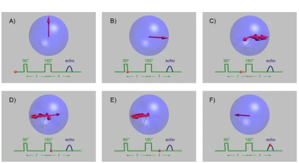
Figure 2.1: Spin echo

A. The spins are first aligned in B⃗⃗⃗0

B. The 90° RF pulse aligns spins in the xOy plane

C. Because of the field inhomogeneities, spins precess with different speeds. D. After a duration 𝑡, a 180° pulse is applied, reversing the spins order E. Because the slower spins are now the first, the fastest ones catch them up F. After a duration 2𝑡, called echo time, spins are realigned in the xOy plane. Image from Wikipedia: https://en.wikipedia.org/wiki/Spin_echo

T1 weighting T2 weighting 𝜌 weighting

White matter White Dark grey Dark grey

Grey matter Grey Light grey Light grey

Cerebrospinal fluid Black White Darker grey

Contrast WM>GM>CSF CSF>GM>WM GM>WM>CSF Table 2.1 Contrast of T1, T2, 𝜌 weighting

2.2

Functional MRI techniques

In this section, we present three of the four main fMRI techniques. The fourth we will introduce is Arterial Spin Labeling (ASL). Since ASL is the core technique of this manuscript, it has its own dedicated chapter afterwards.

2.2.1 Dynamic susceptibility contrast imaging (DSC MRI)

DSC MRI relies on a gadolinium based chelate injected in the subject blood stream. Since the gadolinium compound is paramagnetic, its spreading through the vasculature causes local drops of the signal in T2 (and T2*) weighting with respect to its concentration. Thanks to the kinetic of the gadolinium contrast agent, DSC MRI unlocks the computation of the cerebral blood volume and cerebral blood flow [Østergaard, 2005]. DSC MRI has benefited from a long-time investment of MRI stakeholders, and is currently widely available and easy to use for clinical investigation of the brain perfusion. Less invasive than PET scan, DSC may struggle to compute CBF accurately close to physiological artifact, whether they are pathological or not [Essig et al., 2013]. Note that DSC MRI is the eldest published functional MRI technique [Belliveau et al., 1991].

2.2.2 Dynamic contrast-enhanced MR perfusion (DCE MRI)

Very similar to DSC MRI, DCE MRI also uses gadolinium chelate as contrast agent. However, it uses T1 contrast instead of T2 weighting. In this way DCE MRI can access to some of the microvasculature structure properties like the blood-brain barrier and the vessel permeability. These fine measures of the local perfusion make DCE MRI very effective in the investigation of tumors [Gordon et al., 2014]. Principal downside, DCE MRI implementation and modeling is complex compared to DSC MRI.

2.2.3 Blood-oxygen-level dependent functional MRI

Neural activation leads to a strong local increase in blood flow and an increase in oxygen consumption as discussed in section 1.2. However, the increase in cerebral blood flow is proportionally much higher than the increase in oxygen consumption. The local concentrations of the competing molecules of oxyhemoglobin and deoxyhemoglobin are therefore unbalanced in favor of the oxyhemoglobin. When deprived of its oxygen atoms, hemoglobin possesses "free" iron atoms, whose paramagnetic properties locally induce an increase in the signal (for T2* weighting) due to their decreasing number. It is this small variation (roughly 4% in explained variance) in the signal caused by the disruption of balance that BOLD fMRI tries to capture [Kim and Ugurbil, 1997]. By nature, BOLD fMRI shows its major advantage: it is non-invasive. By allowing therefore the longitudinal investigation of large cohorts of healthy subjects, BOLD fMRI has become and remains the gold-standard for functional MRI. Note that the first human BOLD fMRI experiment was reported just one year after DSC MRI [Ogawa et al., 1992]. However, BOLD fMRI shows an important downside. Indeed, the signal variation captured by BOLD fMRI is multifactorial: it relies on the interaction between the local oxygen concentration, the cerebral blood flow and the cerebral blood volume. Consequently, BOLD fMRI does not report directly the cerebral activity, nor does it allow the computation of the brain perfusion.

2.3

Application: task-based functional MRI

Thanks to the neurovascular coupling, MRI is able to assess neural activity through the hemodynamic response. In the first chapter, we introduced the association between area of the brain and function as one of the functional imaging problematics. In task-based fMRI, the subject is confronted to particular stimuli and/or asked to perform particular tasks, which are called the paradigm in this context. Each stimulus is expected to activate a (or some) corresponding functional area to its nature. For instance, a common task is when the subject is asked to tap a finger from his right hand. In this case, a neural activation in area associated with motor function is expected.

2.3.1 Defining a functional area

Thanks to the linear time invariant property (section 1.3), the variation in signal induced by the stimuli is a priori known, as it is illustrated in Figure 2.3. In order to locate the area of neural activation, task-based fMRI usually models the signal in each voxel as a linear combination of the expected activation signal plus some signals of interference [Poldrack et al., 2011]. By regression, if the linear component associated with the paradigm explains a statistically significant part of the signal variance in the voxel, then the voxel can be assumed to be located in the cerebral area which manage the function corresponding to the paradigm. Note that numerous models have been developed from and beside the widely used linear regression. However, they all involve the expected signal at some point, either to define or to identify the functional area that the paradigm tries to detect.

Figure 2.3: Task-based MRI principle – Illustration with motor area

A subject is exposed to motor stimulus following the black pattern shown in top graph. Thanks to the LTI property, the expected signal in blue is computed from the convolution between the paradigm and canonical HRF. In case 1, the voxel signal in green matches well with the expected signal. It will be considered as belonging to the motor area (in red), unlike the voxel in case 2.

Section 3.

Arterial Spin Labeling

Introduced in 1992 [Detre et al., 1992], Arterial spin labeling (ASL) is the technique of interest of this manuscript. Instead of injecting a radioactive tracer as PET, ASL uses magnetically labelled protons of blood water as an endogenous contrast agent. In this section, we detail some technical aspect on ASL image acquisition and also the cerebral blood flow quantification.

3.1

General principle and declinations of ASL

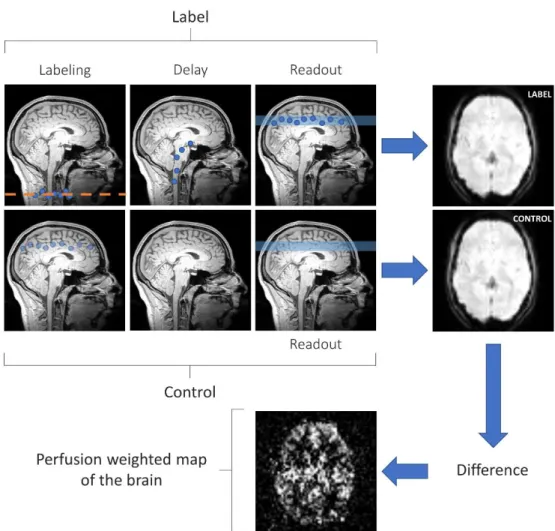
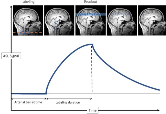
Arterial Spin Labeling is an MRI perfusion technique which uses magnetically labeled arterial water protons as an endogenous tracer. An inversion pulse labels the inflowing blood and after a certain delay, a labeled image of the volume of interest is acquired. The subtraction of the labeled image from a control image, i.e., non-labeled, reflects the quantity of spins that have perfused the imaged volume, producing what is commonly called a perfusion-weighted (PW) image. The PW map can be used to quantify the cerebral blood flow (CBF) under some assumptions [Borogovac and Asllani, 2012; Wang et al., 2012]. Figure 3.1 illustrates these steps in a general framework of an ASL image acquisition. The construction of a label lasts the same duration as the construction of a control, which is called the repetition time (TR)1_{. The label and control steps are repeated}

in order to get numerous PW maps. Depending on the MRI field of investigation, there is two options on how to use the PW maps. On the one hand, one can build an average of the PW maps, which is the topic of basal ASL. As basal ASL builds the average perfusion of the brain map, it focuses more on detection of CBF abnormalities. On the other hand, PW maps can be left as they are, and the investigation can focus on the evolution over time. This declination of ASL, our topic of interest, is called functional ASL. The next sections describe technical aspects of ASL. Functional ASL (fASL), and more generally functional MRI, is also split into two research fields: task-based as we see in in section 3.3. The other research field, resting-state fMRI, is addressed in next section Section 4.

1 _{Some authors consider the TR as the duration of a label plus a control. The description of the}

Figure 3.1: Arterial Spin Labeling generic scheme for image acquisition

Image acquisition is split in two parts: “label” and “control”. In the label part, a RF pulse first aligns the spins of arterial blood water protons in the neck. The labelled protons perfuse then through the brain. After a certain duration called the post-labeling delay, an image is acquired. The signal in label image come from the labelled protons plus the background signal. In the control part, an image is acquitted without labelled protons. Hence, the difference between the labelled image and the control (approximately) remove the background signal. Because the protons spreading is ruled by the cerebral blood flow, the resulting image of the difference is called perfusion weighted image of the brain.

3.1.1 Spin labeling strategy

The labeling consists in sending a RF pulse on the subject neck. It inverts every proton spin in its area of effect. As protons in arterial blood water will perfuse through the brain, they will act hereafter as contrast agent. Mastering this bolus of labelled protons totally relies on the labelling strategy.

Continuous ASL

The oldest method [Williams et al., 1993], the continuous ASL (CASL) strategy consists in the labeling of a thin strip of tissue (1 cm) for a significant period of time, between around 2 s and 4 s. CASL offers a higher covered volume than the other techniques as it is mimicking a real bolus injection of contrast agent which is send to the brain through the vasculature. CASL estimated signal-to-noise ratio is also better than pulsed ASL [Wang et al., 2002], it shows a better resistance to relaxation of spins during the arterial transit time [Parkes and Detre, 2003]. Two major downsides are currently leading to give CASL up for its alternatives. Firstly, the high magnetization transfer of the bolus and its corollary misestimation of the brain perfusion. The second issue is practical: not every MRI device is able to provide such a long labeling radio-frequency pulse.

Pulsed ASL

The pulsed ASL (PASL) instead labels a wide strip of tissue (10 cm) but for a short period duration, around 5 ms. The PASL suffers less from magnetization transfer at the cost of lower estimated signal-to-noise ratio compared to CASL [Wong, 2005]. Plenty of PASL sequences declination and sub-declinations are available depending on which aspect the MRI investigation wants to strengthen: less magnetization transfer (TILT [Golay et al., 1999]), better estimation of axial brain perfusion (PICORE [Jahng et al., 2003]), less sensitivity to arterial transit time (QUIPPS [Wong et al., 1998]).

Pseudo-continuous ASL

In order to combine advantages of PASL and CASL, pseudo-continuous ASL (pCASL) seeks to mimic a CASL labeling by applying a train of rapid radio-frequency pulses [Dai et al., 2008; Silva and Kim, 1999]. Implementable on most MRI devices unlike CASL, pCASL also benefits from a higher signal-to-noise ratio than PASL. Even though the choice of the ASL labeling method can depend strongly on the context, especially when trying to detect activation zones [Borogovac and Asllani, 2012], pCASL is the currently recommended labeling strategy by the “white paper” [Alsop et al., 2015].