UDT and TCP without Congestion Control for Profile Pursuit

(1)

HAL Id: inria-00367160

https://hal.inria.fr/inria-00367160

Submitted on 10 Mar 2009

HAL is a multi-disciplinary open access

archive for the deposit and dissemination of sci-entific research documents, whether they are

pub-L’archive ouverte pluridisciplinaire HAL, est destinée au dépôt et à la diffusion de documents scientifiques de niveau recherche, publiés ou non,

Pursuit

Romaric Guillier, Sébastien Soudan, Pascale Primet

To cite this version:

Romaric Guillier, Sébastien Soudan, Pascale Primet. UDT and TCP without Congestion Control for Profile Pursuit. [Research Report] RR-6874, INRIA. 2009. �inria-00367160�

(2)

a p p o r t

d e r e c h e r c h e

ISRN

INRIA/RR--6874--FR+ENG

Thème NUM

UDT and TCP without Congestion Control for

Profile Pursuit

Romaric Guillier — Sébastien Soudan — Pascale Vicat-Blanc Primet

N° 6874

(3)

(4)

Romaric Guillier , Sébastien Soudan , Pascale Vicat-Blanc Primet Thème NUM — Systèmes numériques

Projet RESO

Rapport de recherche n° 6874 — March 2009 —27pages

Abstract: Instead of relying on the congestion control algorithm and its objective of sta-tistical fair sharing when transfers are assorted with strict deadlines, it might be beneficial to share the links in a different manner. The goal of this research report is to confront two solutions to send data according to a pre-established profile of bandwidth: one based on UDT, one on TCP and PSPacer. In this research report, we have shown how they can be used to implement transfers on such profiles. Based on real experiments a model to predict completion time using RTT and profiles is proposed. For TCP, it is shown to be accurate as soon as the margin is more than 2.5 % of the capacity. Furthermore, the cost of transition is shown to be independent of RTT and height of the steps.

Key-words: Rate Based Transport Protocols, Profile

This text is also available as a research report of the Laboratoire de l’Informatique du Parallélisme http://www.ens-lyon.fr/LIP.

(5)

Résumé : Au lieu de s’appuyer sur un algorithme de contrôle de congestion et son ob-jectif de partage statistique équitable de la bande passante, il pourrait être bénéfique de partager les liens réseaux différamment quand il s’agit d’effectuer des transferts de don-nées constraints par des échéances. Le but de ce rapport de recherche est de confronter deux méthodes permettant d’envoyer des données en suivant un profil de débit pré-défini. La première utilise UDT et la seconde est basée sur TCP et PSPacer. Dans ce rapport de recherche, nous montrons comment ces méthodes peuvent être utilisées pour éxécuter de tels transferts suivant un profil de débit. Un modèle, basé sur des éxpérimentations réelles, est proposé pour estimer le temps de terminaison des transferts en fonction du RTT et du profil appliqué. Pour TCP, nous montrons que ce modèle est précis dès que l’on prend une marge de plus de 2.5 % de la capacité du lien. De plus, nous montrons que le coût des transitions est indépendant du RTT et de la hauteur des transitions.

(6)

1 Introduction

Instead of relying on the congestion control algorithm and its objective of statistical fair sharing, which has been shown to be unpredictable [HDA05], it might be beneficial to share the links in a different manner when transfers are assorted with strict deadlines for example. One of the possible way is to schedule the bandwidth allocated to transfers and try to limit the congestion level.

The goal of this research report is to confront two solutions to send data according to a pre-established profile of bandwidth and find the most suited to perform reliable bulk-data transfers in high-speed shared networks. The first one is based on the UDT implementa-tion of BLAST [HLYD02], and the second one uses TCP with the congestion control part removed combined with PSPacer packet pacing solution.

The rest of the paper is organized as follows: first, we will setup the context of the study by introducing the transport protocols used and their subsequent modifications to allow them to follow a rate profile. Section 3 presents the evaluation methodology that was used. Sections4, 5 and6show the different results we obtained during respectively the calibration, the model-fitting and the model evaluation phases. Finally we conclude in Sect.7.

2 Profile pursuit

This work studies how planned data transfers can be executed. Due to the need of transfer time predictability or resources consumption planning, the considered file transfers have to be done following a given profile. This profile can be a single rate profile or a multi-interval profile giving the bandwidth that can be used during a specified time interval. In the next sections we describe the mechanisms we will use to enforce such a profile.

2.1 Profile pursuit in gridftp

For this study to be fair, it was necessary to use a file-transfer application able to use both TCP and UDT. gridftp suited our needs, but we had to adapt it to follow a profile. The basic idea is to provide gridftp client with a file to transfer and a profile to follow.

To do so, a modified implementation of the UDT xio driver has been implemented. Similarly for TCP, the congestion control mechanism has been modified and a script has been created to configure PSPacer qdisc to follow a profile.

(8)

2.2 Description of modified UDT xio driver

UDT [GG05] is a library built on top of the UDP transport protocol by adding a congestion control scheme and a retransmission mechanism. It was designed to provide an alternative for TCP in networks where the bandwidth-delay product is large.

We have modified the UDT available in the gridftp program so that it follows a rate pro-file: a set of dates according to a relative timer and the corresponding rates that it is allowed to send at. This has been achieved by using the CUDPBlast class of UDT4 implementa-tion and an extra thread which reads the profile file and calls the setRate(int mbps) method on time.

The performance of this version in terms of maximum achievable throughput is strictly identical to the original UDT xio module. It was done so to allow a fair comparison between the TCP and the UDT tests.

2.3 Description of TCP without congestion control

In order to have a profile pursuit mechanism for gridftp with TCP, its congestion control mechanism has been modified to better fill a profile and PSPacer has been used to limit the sending rate.

We briefly describe the modified TCP version used in this paper.

It consists in the normal TCP implementation of TCP in the GNU/Linux kernel with two modifications. First every function of the struct tcp_congestion_ops keeps the congestion window constant by doing:

tcp_sk(sk)->snd_ssthresh = 30000; tcp_sk(sk)->snd_cwnd = 30000;

tcp_sk(sk)->snd_cwnd_stamp = tcp_time_stamp; tcp_sk(sk)->snd_cwnd_cnt = 0;

As a side effect it also removes the slow-start.

Second modification, in function tcp_select_initial_window of the receiver’s kernel, rcv_wnd is not reset to the initial receiver window value (3.mss) when it is too large during the slow-start phase. This enables the sender to send at the maximum rate from the start of the connexion (except before receiving first ACK as the scaling of the advertised receiver window is not possible before).

Basically, it is designed as a hack of the TCP stack that disables the congestion control and sets the congestion control window to a large value. This kind of scheme has already been used in the past [KXK04] and has shown significant improvement over the classical

(9)

congestion control in some situations (lossy links). Similar modifications have been pro-posed by Mudambi et al. under the name of C-TCP in [MZV06]. It is referred throughout this paper as TCP.

To limit the bandwidth used by this TCP without congestion control, the PSPacer kernel module [RTY+₀₅_{] is used. It allows a precise pacing of the packets on the emission site.}

To allow fast transition from a low to high rate, the txqueuelen variable is set to a very large value (100 000 packets) so that packets can be sent upon rate changes without needing to packetise new data.

3 Methodology

The next sections present the methodology and scenarios. The key questions this study tries to answer are the following:

1. Can we use a transport protocol to implement a profile – use all the specified band-width without overflowing?

2. How can we model the performances (bandwidth utilization/goodput)? 3. How can we control the rate to implement a given profile of throughput? 4. Can we predict the completion time of a transfer performed using a profile?

3.1 Testbed

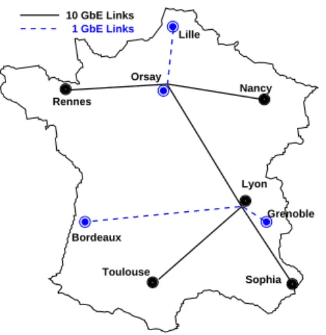
Two different settings were used. The first one is using the Grid’5000 [BCC+₀₆_{] testbed,}

whose simplified topology is shown in Fig. 1. Nodes from the Lyon site and the Rennes site, separated by a 12 ms RTT, are communicating through the 10 Gbps Ethernet backbone network. The bottleneck is the 1 Gbps node (or the output port of the switch just before) that is used as the server. This setting is used in Sect.6of this research report.

The second setting involves a AIST GtrcNet-1 [KKT+₀₄_{], a hardware latency}

emula-tor that is directly connected to two nodes from the Grid’5000 Lyon site. The GtrcNet-1 box is also used to perform precise throughput measurements. This setting is used for the calibration and model fitting part of this research report in sections4and5.

The Rennes nodes are from the paravent cluster (HP ProLiant DL145G2 nodes) and have similar CPU and memory as the Lyon sagittaire nodes (Sun Fire V20z). Both nodes type are 1-Gbps capable.

(10)

Nancy Grenoble Rennes Lille Sophia Toulouse 10 GbE Links Orsay Bordeaux 1 GbE Links Lyon

(11)

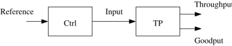
Throughput Goodput Reference Input TP Ctrl Figure 2: Model

3.2 Stage 0 – Preliminary experiments

In order to eliminate potential hardware bottlenecks on the machine, preliminary experi-ments are conducted to evaluate CPU utilization and to compare disk to disk and memory to memory performance of the two alternatives. This is done by measuring the CPU utiliza-tion while sending at a constant rate under different latencies.

For disk to disk and memory to memory performance evaluation, a 7500MB file is transfered at a maximum rate and average rate is measured.

Finally a comparison of performance achieved under different number of parallel flows is done to determine how many flows to use for the remainder of the experiments.

3.3 Stage 1 – Model calibration

3.3.1 Model

In this section, we present the model we use to predict the rates (goodput/throughput) ob-tained from the two different transport protocols for a given input and then to control the throughput to desired value (with an open loop control).

Figure2shows the two blocks of the considered model. TP is transport protocol (along with rate limitation and file serialization mechanisms). It takes as an “input” a rate and gives as an output a “throughput” and a “goodput”. The first one being the bandwidth used on the wire and the second one the transfer rate of the file.

Since UDT and TCP don’t use the same mechanism to control their sending rates and as they have a different packet format, the input signal doesn’t have the same meaning for both of them.

The second block of this model aims at determining the input rate that must be specified to profile enforcement mechanisms to attain the desired throughput. This target throughput is specified by the means of the “reference”. We used throughput-like references (instead of goodput-like) since shared resources, namely the links or bottlenecks, constrain the through-put that the flows can share.

(12)

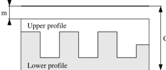
C m

Upper profile

Lower profile

Figure 3: Ideal profiles with link capacity C and margin m.

3.3.2 Scenario for calibration

The goal of the scenarios presented in this section is to evaluate the relation between input rate and goodput and between input rate and throughput.

These scenarios are based on a systematic exploration of input rate space under different RTT for a single rate profile. Input rate ranges from 1 to 1000 Mbps by steps of 1 Mbps. RTT is set to 0 ms, 10 ms, 100 ms and 300 ms. The mean goodput is obtained by dividing the file size by the transfer duration. The mean and maximum instant throughput are measured using GtrcNet-1 which also emulates the latency.

3.4 Stage 2 – Model evaluation

The results from the previous section will provide us with relations between “input” and “goodput”/“throughput”. They will be used to predict the completion time of a transfer under a specified profile. The transfered file has a size of 3200MB.

But before this, this model is used to predict the completion time of a single rate transfer under different RTT and at different rates. The metric used in this scenario is lateness as the model is supposed to predict the completion time.

Two complementary profiles are used in this section. These profiles are presented in Fig.3. It can be noted that a margin m is introduced as a fraction of the bottleneck capacity that none of the flow are supposed to use. We will vary this to evaluate the contention when the profiles are run together. Both profile ends with a steps at the same rate so that both can finish on this step and we can compare the completion time as the average bandwidth allocated to each flow is the same during the first steps.

In order to evaluate the suitability of our model to the profiles, two transfers with com-plementary profiles take place at the same time. Lateness is used to compare the perfor-mances of our prediction under different margins m ranging between 1 and 10% for both

(13)

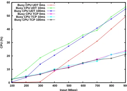
0 10 20 30 40 50 60 100 200 300 400 500 600 700 800 900 CPU (%) Input (Mbps) Busy CPU UDT 0ms

Busy CPU UDT 10ms Busy CPU UDT 100ms Busy CPU TCP 0ms Busy CPU TCP 10ms Busy CPU TCP 100ms

Figure 4: CPU utilization for TCP and UDT as a function of input rate under different latencies.

TCP and UDT. This experiment takes place on an inter-site link of Grid’5000 with 12ms RTT. This latency is not one used to fit the model but is in the range covered by the fitting.

4 Preliminary experiments

4.1 CPU utilization

It can be observed on Fig.4that TCP’s CPU utilization is the same regardless of the latency and that the slope of CPU utilization as a function of input rate is smaller than with UDT. UDT consumes about three times more CPU. But in both cases, CPU is not a bottleneck for the whole range of input rate.

4.2 Memory to Memory

In this test, we use gridftp to tunnel the file /dev/zero from source to the file /dev/null of des-tination. Locally, it has been measured that /dev/zero has a throughput of about 4300 Mbps, which means that our bottleneck will be in the network, not in the node.

(14)

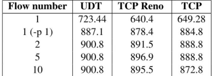
Flow number UDT TCP Reno TCP 1 723.44 640.4 649.28 1 (-p 1) 887.1 878.4 884.8 2 900.8 891.5 888.8 5 900.8 896.9 888.8 10 900.8 895.5 872.8

Table 1: Evolution of the average goodput in Mbps for different transport protocols and number of parallel streams

The cap of performance of TCP can be accounted for (lower than the 941 Mbps limit of a TCP transfer using 1500 bytes MTU over a Gbps Ethernet link) by the cost of using the gridftpapplication. Both TCP variants are able to achieve similar goodputs. UDT is able to perform a little better than TCP, but as the difference is less than 1%, it is then negligible. Same thing for when we are using multiple parallel flows.

When the “-p” option is activated, a multi-threaded version of gridftp is used, which accounts for the fact that we don’t get the same results when we are using only one flow.

4.3 Disk to Disk

In this test, we have pregenerated a large file and we tried to transfer it from nodeA to nodeB. We have observed that every protocol tested averaged to about 360 Mbps. As it corresponds to the speed limits (found through the hdparm tool) of the disk in the nodes, it shows that all these protocols are able to fill up the bottleneck.

Local tests have shown that the differences between D2D and M2M measurements vary very slightly (less than 1 %) when the rate is below the disk’s bottleneck speed1_{. So for the} remaining experiments, we focused on the M2M experiments.

Setting the rate higher than the disk’s bottleneck value is useless and will only lead to suboptimal usage of the networking resources.

5 Model calibration

As seen in the previous section, disk to disk transfer is not interesting as it just adds as an hardware bottleneck. This section will establish the model between input rate, goodput and throughput.

(15)

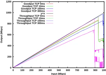
0 200 400 600 800 1000 1200 0 100 200 300 400 500 600 700 800 900 1000 Output (Mbps) Input (Mbps) Goodput TCP 0ms Goodput TCP 10ms Goodput TCP 100ms Goodput TCP 300ms y=x Throughtput TCP 0ms Throughtput TCP 10ms Throughtput TCP 100ms Throughtput TCP 300ms

Figure 5: Goodput and throughput of TCP as a function of “input” rate under different latencies.

5.1 Results

Figures5and6present the mean throughput and the mean goodput obtained by TCP, resp. by UDT, as a function of the input rate for different RTT values.

Even though TCP’s throughput as a function of input rate is below y = x and UDT’s is above, nothing can be concluded from this regarding performance. It simply means that the “input” must be different in order to obtain the same throughput/goodput from them. As we can see that we have straight lines for the most part, we can perform a linear regression to model throughput and goodput as a function of the input rate. This is true for each RTT.

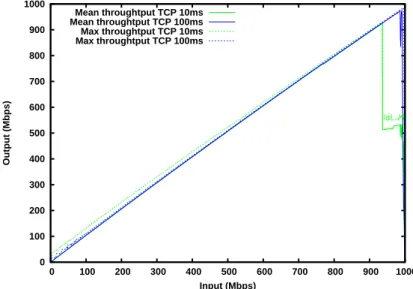
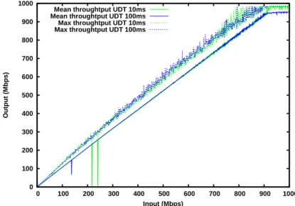
Figures7and8present the mean and max throughput achieved by TCP, resp. UDT. As observed in the previous set of figures, the mean throughput for TCP and UDT are lines, but for TCP the maximum instant throughput is also a straight line, while for UDT it is wildly fluctuating, reaching values larger than 10 % of the mean throughput. This behavior could be problematic when several flows are contending for a bottleneck as, at some instants, UDT can use more bandwidth than in average. It is more bursty than TCP with PSPacer.

For both protocols, the behavior is different for the 300 ms RTT experiment. The GtrcNet-1 box is unable to handle this latency at higher rates, due to the limited buffer size, which leads to packet drops (approximately 10 % loss rate for a 940 Mbps input rate). UDT

(16)

0 100 200 300 400 500 600 700 800 900 1000 1100 0 100 200 300 400 500 600 700 800 900 1000 Output (Mbps) Input (Mbps) Goodput UDT 0ms Goodput UDT 10ms Goodput UDT 100ms Goodput UDT 300ms y=x Throughtput UDT 0ms Throughtput UDT 10ms Throughtput UDT 100ms Throughtput UDT 300ms

Figure 6: Goodput and throughput of UDT as a function of “input” rate under different latencies. 0 100 200 300 400 500 600 700 800 900 1000 0 100 200 300 400 500 600 700 800 900 1000 Output (Mbps) Input (Mbps) Mean throughtput TCP 10ms Mean throughtput TCP 100ms Max throughtput TCP 10ms Max throughtput TCP 100ms

Figure 7: Maximum and mean throughput as a function of input rate for TCP under different latencies.

(17)

0 100 200 300 400 500 600 700 800 900 1000 0 100 200 300 400 500 600 700 800 900 1000 Output (Mbps) Input (Mbps) Mean throughtput UDT 10ms

Mean throughtput UDT 100ms Max throughtput UDT 10ms Max throughtput UDT 100ms

Figure 8: Maximum and mean throughput as a function of input rate for UDT under differ-ent latencies.

seems to be deeply affected by this as the mean throughput doesn’t go above 320 Mbps. TCP behavior doesn’t change until the input/throughput reaches 900 Mbps.

This can be explained by the fact that UDT generates bursts at a much higher rate than the input value, leading to heavy losses in this case. These bursts don’t exist for TCP as PSPacer is used to limit and pace the throughput on the emitter. The slight change of slope for the UDT goodput at 300 ms RTT is due to the use of a timeout to limit the duration of one transfer.

The modelling presented in the following section takes this problem into consideration as we restricted the fitting over the linear parts.

5.2 Model fitting

In this section, we model the mean throughput and goodput obtained in the previous section as a function of the RTT and of the input rate X. This model is necessary as we need to find out for each protocol which input rate to provide so as to get a given throughput.

Since we observed a linear behavior of the throughput and of the goodput, we use a linear regression to fit the model:

(18)

goodput(X, RT T ) = ag(RT T ) ∗ X + bg(RT T ) (1)

throughput(X, RT T ) = at(RT T ) ∗ X + bt(RT T ) (2)

From that, we can write the input X as a function of throughput or goodput: X= throughput(X, RT T ) − bt(RT T ) at(RT T ) (3) X= goodput(X, RT T ) − bg(RT T ) ag(RT T ) (4) Finally, we can express throughput (resp. goodput) as a function of goodput (resp. throughput): throughput(X, RT T ) = at(RT T ) ag(RT T )(goodput(X, RT T ) − b g(RT T )) + bt(RT T ) (5) goodput(X, RT T ) = ag(RT T ) at(RT T ) (throughput(X, RT T ) − bt(RT T )) + bg(RT T ) (6)

It is this formula that will be used throughout of the rest of this research report to gen-erate the appropriate values for the profile.

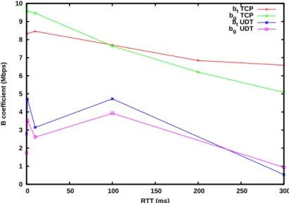
The resulting coefficients are shown in Fig. 9 and 10. As these coefficients are still depending on the RTT, we also need to model them as a function of RTT. As in Fig.9, the relationship between the coefficients and the RTT seems to be linear, we perform another linear regression.

The resulting final model is rather good for TCP as the correlation coefficients are above 0.99 for the goodput and above 0.98 for the throughput. The modelling obtained for UDT is less accurate, especially for the b coefficients, but as they are rather small, we can assume that the impact will be limited for large target throughput values.

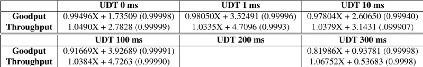
Tables 2and3 provide the actual values of the coefficient computed. Tables4 and5

(19)

0.75 0.8 0.85 0.9 0.95 1 1.05 1.1 0 50 100 150 200 250 300 A coefficient RTT (ms) at TCP ag TCP at UDT ag UDT

Figure 9: agand atfor TCP and UDT as a function of RTT.

0 1 2 3 4 5 6 7 8 9 10 0 50 100 150 200 250 300 B coefficient (Mbps) RTT (ms) bt TCP b_g TCP bt UDT b_g UDT

(20)

UDT 0 ms UDT 1 ms UDT 10 ms

Goodput 0.99496X + 1.73509 (0.99998) 0.98050X + 3.52491 (0.99996) 0.97804X + 2.60650 (0.99940)

Throughput 1.0490X + 2.7828 (0.99999) 1.0335X + 4.7096 (0.9993) 1.0379X + 3.1431 (.099907)

UDT 100 ms UDT 200 ms UDT 300 ms

Goodput 0.91669X + 3.92689 (0.99991) 0.81986X + 0.93781 (0.99998)

Throughput 1.0384X + 4.7263 (0.99990) 1.06752X + 0.53683 (0.9998)

Table 2: Goodput and Throughput as a function of the input X and correlation coefficient for UDT TCP 0 ms TCP 1 ms TCP 10 ms Goodput 0.93280X + 9.56543 (0.99974) 0.93203X + 9.56445 (0.99974) 0.91939X + 9.46380 (0.99974) Throughput 0.99110X + 8.33749 (0.99988) 0.99111X + 8.33450 (0.99988) 0.99099X +8.45958 (0.99988) TCP 100 ms TCP 200 ms TCP 300 ms Goodput 0.87199X + 7.64142 (0.99982) 0.81791X + 6.20263 0.77160X + 5.08259 (0.99988) Throughput 0.99163X + 7.69914 (0.9990) 0.99234X + 6.84330 (0.99985) 0.99365X + 6.58520 (0.99992)

Table 3: Goodput and Throughput as a function of the input X and correlation coefficient for TCP

UDT a(RTT) UDT b(RTT)

Goodput -5.599518e-4RTT + 0.984038 (-0.99353) -0.00517RTT + 2.971245 (-0.538542)

Throughput 8.904223e-5RTT + 1.037945 (0.837839) -0.009606RTT + 3.96935 (-0.71783)

Table 4: Linear regression coefficients as a function of RTT for UDT

TCP a(RTT) TCP b(RTT)

Goodput -5.36746e-4RTT + 0.928945 (-0.998147) -0.015479RTT + 9.496315 (-0.994341)

Throughput 8.155708e-6RTT + 0.990973 (0.982622) -0.006467RTT + 8.368437 (-0.98429)

(21)

-3.5 -3 -2.5 -2 -1.5 -1 -0.5 0 0 0.01 0.02 0.03 0.04 0.05 0.06 0.07 0.08 0.09 0.1 Lateness (s) Margin (%) TCP 0ms RTT 500Mbps TCP 10ms RTT 200Mbps TCP 10ms RTT 500Mbps TCP 10ms RTT 800Mbps TCP 100ms RTT 200Mbps TCP 100ms RTT 500Mbps TCP 100ms RTT 800Mbps

Figure 11: Verification of the model using lateness on a simple constant profile for TCP.

-3 -2 -1 0 1 2 3 4 5 6 7 0 0.01 0.02 0.03 0.04 0.05 0.06 0.07 0.08 0.09 0.1 Lateness (s) Margin (%) UDT 0ms RTT 500Mbps UDT 10ms RTT 200Mbps UDT 10ms RTT 500Mbps UDT 10ms RTT 800Mbps UDT 100ms RTT 200Mbps UDT 100ms RTT 500Mbps UDT 100ms RTT 800Mbps

(22)

5.3 Model validation on single rate profile

Finally, we check the validity of the model over a simple case scenario. A constant profile is defined for different RTTs and target throughputs for a transfer that is expected to last about 60 s. The results are averaged over 10 tries. Figures11and12show the lateness on these experiments where m lies between 0 and 10% by steps of 0.5% for both TCP and UDT.

It seems to performs well for TCP as the results are never over the estimated completion time and most of the time the difference is less than one second. Adding a margin doesn’t significantly improve the prediction for TCP.

The results are not as good for UDT, especially for the small values for the target throughput and large latency (200Mbps and 100ms RTT). That is probably due to the con-stant coefficients the model of which isn’t accurate enough. With a reasonable margin, however, it is possible to get close enough to the estimated completion time.

This also shows that the roundings performed for the purpose of the generation of the profile don’t affect the results much. Computations show that the rounding would cause a difference in completion time of about 100 ms, which is significantly smaller than 60 s.

6 Model evaluation

In this section, we are studying the impact of sharing a bottleneck using steps profile as defined in Sect.3and comparing predicted completion times using the model established in Sect.5.

Figure13shows the typical behavior of the TCP and the UDT throughput when follow-ing a step profile. For instance, we can see that there is a time-lag between the moment a change of rate is asked and the moment it is really enforced.

6.1 Two profiles, margin & lateness

Figure14shows the lateness of the two transfers using the profile defined above for TCP and UDT with a 12ms RTT. It can be noted that TCP performs very well as soon as the margin is high enough to prevent losses. This threshold lies at 2.5 % of margin. Concern-ing UDT, we can observe that there is no such threshold and that the lateness decreases smoothly until 25 %, where it reaches 1 s. This is probably related to Fig.7and8where the maximum instant throughput is shown. UDT’s max throughput was always well above the mean throughput.

In Fig.15, a similar experiment is conducted except that the two competing flows are using a different protocol. Here we can observe that the TCP flow is deeply impacted as the

(23)

0 200 400 600 800 1000 10 15 20 25 30 35 40 45 50 Throughput (Mbps) Time (s) Reference steps TCP steps UDT steps

Figure 13: TCP and UDT steps of throughput compared to reference profile.

-10 0 10 20 30 40 50 60 70 0 5 10 15 20 25 Lateness (s) Margin (%) TCP upper TCP lower UDT upper UDT lower

Figure 14: Lateness (95% confidence interval) as a function of margin m for a 60s transfers using TCP and UDT for 12ms RTT.

(24)

-20 -10 0 10 20 30 40 50 60 0 5 10 15 20 25 Lateness (s) Margin (%) TCP UDT

Figure 15: Lateness (95% confidence interval) as a function of margin m for a 60s transfers using TCP for one and UDT for the other for 12ms RTT.

lateness is never under 10 s. Meanwhile, the UDT flow doesn’t experience any delay when the margin is more than 2.5 %.

6.2 Transitions

In order to explain the remaining lateness, we take a look at the step transitions.

To allow a better understanding of this phenomenon, a close up of the throughput dur-ing the transition from 10 Mbps to 600 Mbps is shown in Fig.16. The area between the TCP/UDT throughput and the step shape corresponds to a volume of data that couldn’t be sent.

Figure13seems to point out that what we are losing on the increasing side is gained on the decreasing side of the steps or even through the UDT bursts, but we are trying to provide a upper bound for that.

Figures17(b)and17(c)present the cost in time of a transition from a low value (10 Mbps) to a high value for different RTT values for TCP, resp. UDT. It is a part of the profile where we are very likely to lose time due to the necessity to adapt to the new throughput value. We can see that the cost doesn’t depend much on the RTT and that it can be bounded by a few tens of milliseconds. It is significantly smaller than the overall duration of the transfer.

(25)

0 100 200 300 400 500 600 700 800 0.35 0.4 0.45 0.5 0.55 0.6 0.65 Throughput (Mbps) Time (s) Reference steps TCP steps UDT steps

Figure 16: TCP and UDT steps of throughput compared to reference profile (Close up) for a 10–600Mbps step.

This is all the more obvious when compared to TCP Reno17(a). In this case, we can see that the cost linearly increases with the height of the transition, due to the AIMD congestion avoidance algorithm increases the congestion window linearly. We can also see the impact of the RTT feedback loop, as the cost dramatically increases with the RTT to be about 1 s per transition for a 100 ms RTT. Using TCP Reno to follow a bandwidth profile seems inadequate as soon as the RTT is above local range (about 0.1 ms).

The main cause of the observed lateness is probably due to synchronization problems between the two emitters: a look at the gridftp server log shows that there is in average about 200 ms difference at the connection start-time, which might enough to upset the whole sharing of the bandwidth. In this case, applying a small margin is then the solution to guarantee a completion in time for all the transfers.

7 Conclusion

In this research report, we have shown how UDT and TCP without congestion control+pacing can be used to implement transfers on a profile of rate. The affine models proposed to predict the completion time is a function of RTT and throughput of the profile. Model is accurate

(26)

0.01 0.1 1 10 0 200 400 600 800 1000 Lateness (s) Transition height (Mbps) TCP reno 0ms RTT TCP reno 12ms RTT TCP Reno 100ms RTT (a) TCP Reno 0 0.005 0.01 0.015 0.02 0.025 0.03 0 200 400 600 800 1000 Lateness (s) Transition height (Mbps) TCP 0ms RTT TCP 12ms RTT TCP 100ms RTT (b) TCP 0 0.005 0.01 0.015 0.02 0.025 0.03 Lateness (s) UDT 0ms RTT UDT 12ms RTT UDT 100ms RTT RR n° 6874

(27)

for TCP as soon as the margin is more than 2.5% of the capacity. However, the model is less accurate for UDT as its throughput is more bursty. This causes the instant throughput to be significantly higher than the predicted mean throughput. Still, the lateness is less than 1s on 60s transfers when margin is higher than 15%. We also showed that the cost of transition is independent of RTT and steps’ height. This cost, expressed in term of lateness, has been evaluated to be between 10ms and 20ms each.

This model and enforcement mechanisms can be used as a part of a scheduled transfer solutions.

8 Acknowledgments

This work has been funded by the French ministry of Education and Research, INRIA (RESO and Gridnets-FJ teams), via ACI GRID’s Grid’5000 project, the IGTMD ANR grant, NEGST CNRS-JSP project. A part of this research was supported by a grant from the Ministry of Education, Sports, Culture, Science and Technology (MEXT) of Japan through the NAREGI (National Research Grid Initiative) Project and the PAI SAKURA 100000SF with AIST-GTRC.

(28)

List of Figures

1 Grid’5000 topology . . . 7

2 Model . . . 8

3 Ideal profiles with link capacity C and margin m. . . 9

4 CPU utilization for TCP and UDT as a function of input rate under different latencies. . . 10

5 Goodput and throughput of TCP as a function of “input” rate under different latencies. . . 12

6 Goodput and throughput of UDT as a function of “input” rate under differ-ent latencies. . . 13

7 Maximum and mean throughput as a function of input rate for TCP under different latencies.. . . 13

8 Maximum and mean throughput as a function of input rate for UDT under different latencies.. . . 14

9 agand atfor TCP and UDT as a function of RTT. . . 16

10 bgand btfor TCP and UDT as a function of RTT. . . 16

11 Verification of the model using lateness on a simple constant profile for TCP. 18

12 Verification of the model using lateness on a simple constant profile for UDT. 18

13 TCP and UDT steps of throughput compared to reference profile. . . 20

14 Lateness (95% confidence interval) as a function of margin m for a 60s transfers using TCP and UDT for 12ms RTT. . . 20

15 Lateness (95% confidence interval) as a function of margin m for a 60s transfers using TCP for one and UDT for the other for 12ms RTT. . . 21

16 TCP and UDT steps of throughput compared to reference profile (Close up) for a 10–600Mbps step. . . 22

17 Cost of low to high transition in term of loss of time . . . 23

List of Tables

1 Evolution of the average goodput in Mbps for different transport protocols and number of parallel streams . . . 11

2 Goodput and Throughput as a function of the input X and correlation coef-ficient for UDT . . . 17

3 Goodput and Throughput as a function of the input X and correlation coef-ficient for TCP . . . 17

(29)

(30)

References

[BCC+_{06] Raphaël Bolze, Franck Cappello, Eddy Caron, Michel Daydé , Frederic}

Desprez, Emmanuel Jeannot, Yvon Jégou, Stéphane Lanteri, Julien Leduc, Noredine Melab, Guillaume Mornet, Raymond Namyst, Pascale Vicat-Blanc Primet, Benjamin Quetier, Olivier Richard, El-Ghazali Talbi, and Touché Irena. Grid’5000: a large scale and highly reconfigurable experimental Grid testbed. International Journal of High Performance Computing Applications, 20(4):481–494, Nov. 2006.

[GG05] Yunhong Gu and Robert L. Grossman. Supporting Configurable Congestion

Control in Data Transport Services. In SuperComputing, November 2005. [HDA05] Qi He, Constantinos Dovrolis, and Mostafa H. Ammar. Prediction of TCP

throughput: formula-based and history-based methods. In Sigmetrics. ACM, 2005.

[HLYD02] E. He, J. Leigh, O. Yu, and T.A. Defanti. Reliable blast udp : predictable high performance bulk data transfer. Cluster Computing, 2002. Proceedings. 2002 IEEE International Conference on, pages 317–324, 2002.

[KKT+_{04] Y. Kodama, T. Kudoh, R. Takano, H. Sato, 0. Tatebe, and S. Sekiguchi.}

GNET-1: Gigabit Ethernet Network Testbed. In International Conference on Cluster Computing. IEEE, Sept. 2004.

[KXK04] R. Kempter, B. Xin, and S. K. Kasera. Towards a Composable Transport Pro-tocol: TCP without Congestion Control. In SIGCOMM. ACM, August 2004. [MZV06] A.P. Mudambi, X. Zheng, and M. Veeraraghavan. A transport protocol for

dedi-cated end-to-end circuits. Communications, 2006. ICC ’06. IEEE International Conference on, 1:18–23, June 2006.

[RTY+_{05] R.Takano, T.Kudoh, Y.Kodama, M.Matsuda, H.Tezuka, and Y.Ishikawa.}

De-sign and Evaluation of Precise Software Pacing Mechanisms for Fast Long-Distance Networks. In PFLDnet, Feb. 2005.

(31)

Unité de recherche INRIA Futurs : Parc Club Orsay Université - ZAC des Vignes 4, rue Jacques Monod - 91893 ORSAY Cedex (France)

Unité de recherche INRIA Lorraine : LORIA, Technopôle de Nancy-Brabois - Campus scientifique 615, rue du Jardin Botanique - BP 101 - 54602 Villers-lès-Nancy Cedex (France)

Unité de recherche INRIA Rennes : IRISA, Campus universitaire de Beaulieu - 35042 Rennes Cedex (France) Unité de recherche INRIA Rocquencourt : Domaine de Voluceau - Rocquencourt - BP 105 - 78153 Le Chesnay Cedex (France)