HAL Id: hal-02171480
https://hal.archives-ouvertes.fr/hal-02171480v3
Preprint submitted on 16 Dec 2019HAL is a multi-disciplinary open access archive for the deposit and dissemination of sci-entific research documents, whether they are pub-lished or not. The documents may come from teaching and research institutions in France or abroad, or from public or private research centers.
L’archive ouverte pluridisciplinaire HAL, est destinée au dépôt et à la diffusion de documents scientifiques de niveau recherche, publiés ou non, émanant des établissements d’enseignement et de recherche français ou étrangers, des laboratoires publics ou privés.
The Ups and Downs of European Real Estate Markets’
Integration
Jean-François Carpantier, Christelle Sapata
To cite this version:
Jean-François Carpantier, Christelle Sapata. The Ups and Downs of European Real Estate Markets’ Integration. 2019. �hal-02171480v3�
The Ups and Downs of European Real Estate
Markets’ Integration
∗
Jean-François Carpantier and Christelle Sapata
†December 16, 2019
Abstract
National real estate markets are usually considered to be segmented from each other. The benefits of international diversification in real estate markets have been shown to be greater than those in equity or bond markets. New developments in Europe (the single market, monetary union and post-crisis coordination of macroprudential policies) are expected to increase integration and reduce these benefits. We study the time-varying degree of integration of European real estate markets over the period 1971-2017 by esti-mating the explanatory power of a multi-factor linear model. We find that the integration has been relatively stable over time, with a temporary rise during the 2008 financial cri-sis. We also note that the integration dynamics within Europe have not become stronger than with non-European countries. The data do not detect stable regional clusters of integration. The international diversification of real estate investments still matters.
Introduction
The integration of international financial markets has increased over time, but real estate as-sets have long been considered to be segmented, both with respect to equity or bond markets, and across countries. For a real estate investor, geographic diversification has been shown to be profitable (see for empirical examples Eichholtz (1996), Lee (2005) or de Wit (2010)). As noted in the conclusion of de Wit (2010), "investing in assets across regions will result in the highest diversification benefits".
∗We would like to thank the editor and two anonymous referees, who provided valuable suggestions and comments. This research was conducted as part of the research program entitled "Risk Management and Investment Strategies” under the aegis of the Europlace Institute of Finance and Insti7.
†Aix-Marseille University, Cergam EA 4225, [email protected],
These benefits have however been questioned recently. First, some international studies (Case et al. (2000), Cotter et al. (2015), Joyeux and Milunovich (2015)) have shown a re-cent rise in the integration of national housing markets, especially during crisis episodes. Second, the introduction of the euro and the resulting common monetary policy, together with the growing coordination of macroprudential policies in the wake of the 2008 crisis are candidates for supporting the integration of housing markets. Whether this is a perma-nent or temporary rise and whether geographic diversification still matters remain unresolved questions that we investigate in this paper.
This question is also motivated by the growing importance of real estate investments in the world. According to a recent MSCI report, the professionally managed global real estate investment market grew by 10% in 2017, reaching USD 8.5 trillion, a large figure compared with sovereign wealth fund assets (USD 8 trillion) and hedge fund assets (around USD 3.5 trillion). Although not specific to Europe, the growing financialization of the real estate market is certainly another potential source of (ongoing) market integration.
We study here the time-varying integration of the European real estate markets over the period 1971-2017, based on national return series, as collected and harmonized by the Bank for International Settlements (BIS). Our measure of time-varying integration is based on the contribution of Pukthuanthong and Roll (2009). It is captured by the explanatory power, that is, the adjusted R2, of a multi-factor model, in which the dependent variables are the annual
variations of housing price series and the explanatory variables are the unobserved common sources of variations in the European housing market. These common sources of variation are captured by factors obtained via principal component analysis. In terms of interpretation, a high adjusted R2 means that the common sources of variation explain a large part of the national housing price variations; in other words, a high degree of integration exists. Since we want to measure it dynamically and determine how integration changes over time, we replicate this analysis with a set of consecutive sub-samples of 6 years (overlapping rolling windows). We discuss our results both at the national level by considering the evolution of national-specific measures of integration and globally with the European time-varying integration by averaging our results.
We find that European real estate markets are now more integrated than previously, but we also realize that this higher level of integration is quasi exclusively due to a temporary shift associated with the 2008 crisis. We also find that the within-Europe integration is not stronger than the integration of European housing markets with non-European factors. In addition, we document the instability of regional clusters, further supporting the low degree of integration. Clearly, the benefits of geographic diversification still matter for European markets.
This paper is organized as follows. First, we review the literature on the integration measures and the empirical results regarding the integration of European real estate markets. We then explain our estimation strategy. The third section presents our data and the fourth one the results. We then propose some extensions by comparing the integration within Europe and the integration with non-European countries, and consider a regional clustering approach. Finally, the last section concludes.
1
Review of literature
1.1
Measures of integration
We cover some of the perspectives behind the concept of integration in this subsection. We first discuss convergence versus synchronization, then we look at the different usual proxies (prices, quantity and regulations) and finally we present static versus dynamic measures of integration.
1.1.1 Convergence versus synchronization
We investigate the benefits of diversification by studying the integration of the European housing markets over time. There is, however, no unique consensual definition of integra-tion. Everything depends on the perspective and on the final question that is raised. There are basically two perspectives: one on levels and the other on dynamics. The first perspective sees integration as a convergence process whereby real estate markets start from different initial conditions (say different price levels). The analysis then assesses the existence and speed of a convergence process (see for illustration McAllister (2001), who estmated the integration through beta convergence, or Gallo et al. (2013), who estimated it in a cointegra-tion framework). The second perspective rather considers integracointegra-tion as a synchronizacointegra-tion dynamic process, in which the focus is on exposure to common factors and on co-movements and correlations. Although convergence and synchronization might go hand in hand, this is not necessarily the case. Indeed, a recent study (Jeffrey et al. (2018)) showed at the euro area level that the European real economic activity has not converged even though the fluc-tuations have become increasingly synchronized. There is a priori no reason to consider that this divide would be different for real estate markets.
Since we have no hedonic price series (correcting for quality levels across countries) allow-ing us to assess the genuine convergence of markets, we look at integration in terms of syn-chronicity. This is also the most natural approach, as we take the perspective of an investor concerned about the diversification benefits of investing in different European countries.
1.1.2 Prices, quantities or regulations
As detailed in Billio et al. (2017), we can assess integration by looking at price measures (returns, rents or yields), but other objects of study could also be considered. As the first alternative, we can use a quantity indicator that refers to stocks or flows of real estate. Full integration requires internationally diversified portfolios. For instance, one could measure integration through the share of real estate held by domestic with respect to foreign resi-dents. As the stock of real estate held by foreign residents increases, the impact of domestic idiosyncratic shocks decreases. In terms of flows, one could analyse the share of real estate transactions carried out by residents or non-residents. A third approach to integration could
be to study the harmonization of regulations. Sharing the same regulations can facilitate the integration of European markets even though it may not be a sufficient condition for integra-tion. In this respect, integration in real estate would appear to be limited, as property rights have so far not been subject to a specific EU directive. As we consider the integration of real estate markets from a financial diversification viewpoint, we adopt a return perspective.
1.1.3 Dynamic versus static
We consider the evolution of the integration and therefore rely on dynamic measures as op-posed to static ones. Different tools can be used for estimating the time-varying integration, such as multivariate volatility models (CCC, DCC and BEKK-GARCH) or time-varying beta models (see Billio et al. (2017) for a recent survey). Nevertheless, most of these measures are subject to the criticism of Pukthuanthong and Roll (2009), who stated that: "Correlations can be small even when two countries are perfectly integrated. This occurs whenever there are multiple global sources of return volatility and countries do not share the same sensitivities to all of them." They therefore suggested using a multi-factor model in which the integration of the real estate return series is measured through the time-varying explanatory power of the global factors. If that proportion is small, the country is dominated by local or idiosyncratic influences, but, if a group of countries is highly sensible to the same global influence, there will be a high degree of integration.
Two advantages of this approach are first that the analysis does not require us to choose observable global factors - these are latent factors - and second that we obtain a measure of integration that is comparable over time, as the change in the R2 indicates the change in the
market integration. This quite novel approach has been implemented by Pukthuanthong and Roll (2009) for the equity market, by Christoffersen et al. (2019) for commodity markets and by Cotter et al. (2015), who related their dynamic measure to specific macro and financial variables.
1.2
Integration of European real estate markets
We are not the first to study the integration of European real estate markets. Druica et al. (2015) used proxy measures of returns and rental yields in residential real estate in Europe and explored the correlation of these variables with factors such as the GDP, population and inflation. They found that the same structural factors drive real estate returns. Bond et al. (2003) showed that commercial real estate markets are fragmented. They used a multi-factor international asset pricing model and presented evidence of a strong global risk factor in almost all real estate sectors. The diversification benefits of real estate have thus been con-firmed, but it appears to be more relevant in Asia-Pacific markets than in European markets. Still, these papers focused on static statistics, contrary to our approach, which is based on the evolution of the housing real estate market integration.
conver-gence, which summarizes the evolution of distribution over time. There is integration accord-ing to sigma convergence when the dispersion in the distribution falls over time. McAllister (2001) used sigma convergence on RE rental prices in the office market and found no evi-dence of sigma convergence when applied to the office rents of 25 cities in Europe between 1984 and 1999. However, with a larger time scope (1982-2009), Srivatsa and Lee (2010) found significant sigma convergence, but their sample was smaller, with only 7 European office markets.
Some papers have adopted a country-specific focus and considered the time-varying integra-tion with other European countries. Lee (2009) showed that the returns of the UK securitised real estate market were influenced more by the fluctuations in European markets than by those in the US market between 1998 and 2004. However, since 2004, he noted that the real estate returns in the UK have started to diverge from those of most countries in Europe. Lee (2010) replicated his method with the Spanish real estate market and showed that there is evidence of convergence with some European countries but not all of them, suggesting that diversification of portfolios within Europe is still viable but the choice of country is crucial. To sum up, no paper has analysed the evolution of the integration of European real estate
markets. The residential market has been analysed from a static perspective, and the results have shown no evidence of integration. Then, the dispersion of price variations of the office market has decreased, signalling some degree of sigma convergence but not necessarily of integration. Finally, studies that have tested the integration of national real estate markets with respect to the rest of Europe have tended to obtain only weak evidence of integration.
2
Methodology
This section describes the methodology employed to measure the time-varying degree of integration of European real estate markets.
2.1
Benchmark model
As standard correlation coefficients are not designed for disentangling low integration from large heterogeneity1, we opt for an alternative approach whereby integration is measured
us-ing the explanatory power of a multi-factor linear model in which the dependent variables are annual variations of housing price series and in which the factors, as explanatory variables, capture the key driving sources of variation in the global housing market. This approach follows Pukthuanthong and Roll (2009), who implemented this methodology to assess the rising integration of equity markets.
The factors used in this methodology are obtained by computing the principal components
1Well-integrated countries could have low correlations if they do not have the same sensitivities to global sources of variations.
from the spectral decomposition of the correlation matrix of the annual percentage variations in our housing price series. More formally, the factors are computed as follows:
Fk,t= ek,1r1,t+ ... ek,iri,t+ ... ek,NrN,t (1)
i = 1, ... N k = 1, ... K t = 1, ... T
where N is the number of housing price series (i.e. the number of countries), K < N is the number of factors, T is the size of the time series, Fk,t is the factor (i.e. principal
component) k at time t, ek,iis the i-th element of the N -dimensional eigenvector associated
to the principal component k (and to the eigenvalue λk), ri,tis the annual percentage variation
of the real estate quarterly price series of country i in year t.
Equation 1 shows that the factors are built as linear combinations (or weighted "averages" where PN
i=1e 2
k,i = 1 ∀k) of the housing returns. These factors are used as proxies for
common sources of variation and are therefore included as explanatory variables in the N multi-factor regressions implemented separately for each real estate national market:
ri,t = βi,1F−i,1,t+ ... βi,kF−i,k,t+ ... βi,KF−i,K,t (2)
−i = 1, 2 ..., i − 1, i + 1, ..., N
where βi,k is the country i exposure (or factor loading) to the global factor k, where the
sub-script −i in F−i,k,texplicitly shows that the global factors in the country i-specific regression
are computed without consideration of the real estate returns of country i. If country i real estate returns were not excluded from the computation of the global factors specific to regres-sion i, the explanatory power of the country i regresregres-sion would artificially be biased upward, with a magnitude depending on the weight of country i returns in the set of the K global factors considered in the regressions. We thus first compute for the country i regression a set of K different factors based on their repective N − 1 return series and then regress the country i return on this set of K factors; finally, we repeat this procedure for the N countries of the sample.
The (adjusted) R2s obtained from the above regressions are then averaged over countries
and give the key outcome for assessing the degree of integration of the European housing market. However, the averaged R2 is a single figure summarizing the degree of integration of the N real estate markets in the full sample. Our objective was to make it dynamic (time-varying) with the aim of addressing our research question concerning the evolution of real estate markets’ integration. We thus follow Billio et al. (2017) and estimate the cross-country averaged R2 using a rolling window of 6 years. As detailed in the data section, the
time coverage of our data extends from 1971q1 to 2017q4. Wel thus ultimately obtain a set of 160 cross-country averaged R2s showing the evolution of the explanatory power of global factors, in other words the degree of integration of housing markets over time.
2.2
Implementation "details"
The devil is often in the detail in such studies. Our analysis requires us to make a set of arbi-trary assumptions about the object of the spectral decomposition (correlation or covariance
matrix), the handling of potential non-stationarity and seasonality of the data, the considera-tion of potential time-delayed integraconsidera-tion, the size of the rolling window and the number of global factors. We now discuss carefully these important technical points, which can, in the end, make a big difference.
First, the spectral decomposition of a matrix allows us to compute/isolate its eigenvectors and associated eigenvalues. We can operate the decomposition either on the covariance matrix or on the correlation matrix of the real estate returns. Using the covariance matrix consists of allocating different weights to the series, the magnitude of which is commensurate with their respective variances. Since there is no reason to expect a larger influence on global factors of a highly volatile country - actually we would expect the contrary - we work on a correlation matrix (like Billio et al. (2017)). Using the correlation matrix is actually equivalent to working with the covariance matrix of the standardized returns.
Second, the spectral decomposition requires the series to be stationary. Given the non-stationarity resulting from standard non-stationary tests, we work with returns instead of prices, as is usual in similar studies. We also notice some country-specific seasonality in the data (resulting from tax, weather or job market specificities, among others). We thus work with annual percentage variations in our quarterly price series. An alternative might be to rely on deseasonalization tools (such as the X11 filter), but this would be at the cost of a loss of transparency. In the robustness section, we report a comparison with quarterly variations (instead of annual ones).
Third, the global factors are constructed on the basis of the correlation matrix, which only reflects contemporaneous correlations between real estate markets. However, real estate mar-kets are characterized by some rigidities that preclude instantaneous (and full) reflections of global shocks. Limiting our measure of integration to the sole contemporaneous correlation with global factors is too restrictive. We thus consider a model that allows some delay in the shock’s propagation. We add lagged factors to our benchmark model. Formally,
ri,t =βi,1F−i,1,t+ ... βi,kF−i,k,t+ ... βi,KF−i,K,t+ (3)
βi,10 F−i,1,t−1+ ... βi,k0 F−i,k,t−1+ ... βi,K0 F−i,K,t−1
where the additional K factors F−i,k,t-1are lagged factors accounting for a potential quarterly
delay. We also explore the sensitivity of our results by comparing different variants of our model (no lag, two lags, three lags).2
Fourth, we estimate the cross-country averaged R2 using a rolling window of 6 years. The
longer the rolling window, the longer the sample and the more precise the estimate. The shorter the window, the more reflective it is of the current degree of integration. Given this trade-off, we also compare our results by varying the length of the rolling window (six, eight and ten years, respectively). This also helps in documenting the degree of persistence of the 2008 financial crisis in the time-varying R2measure.
Finally, the number of factors, K, to be included as explanatory variables is determined
2Alternatively, Pukthuanthong and Roll (2009) computed factors by augmenting the covariance matrix with one-quarter-lagged returns.
by stating that the cumulative proportion of total variance, (PK
k=1λj)/(
PN
k=1λj) (where
λk stands for the kth largest eigenvalue resulting from the spectral decomposition of the
correlation matrix), explained by the K factors, must reach the threshold of 80%. We also explore the sensitivity of this assumption (three, four and five factors respectively).
3
Data
3.1
Data sources
The BIS publishes a so-called long series data set on residential property prices, which fo-cuses on 18 advanced economies with historical data that reach as far back as 1971 on a quarterly basis (Scatigna et al. (2014)). The selected series cover all types of dwelling (flats and houses, new and existing). According to the BIS, this indicator "satisfies some minimum comparability criteria across countries", "without, however, fully eliminating all discrepan-cies" (Scatigna et al. (2014)).3
The dataset covers 13 European countries, consisting of 11 EU ones (Belgium, Finland, Denmark, France, Germany, Ireland, Italy, the Netherlands, Spain, Sweden and the United-Kingdom (still in the EU at the time of writing)) and 2 non-EU countries, Norway and Switzerland.4 It also covers 5 non European countries, namely Australia, Canada, Japan, New Zealand and the United States, which we use as a comparison group in Section 5. The time coverage extends from 1971q1 to 2017q4, that is, over 188 quarters.
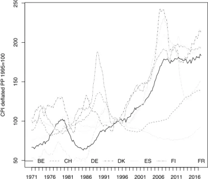
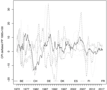
The BIS property price series that we use are expressed in nominal terms. The series are therefore deflated with the consumer price indices from the World Bank dataset. 5 Figures 1 and 2 illustrate the evolution of our 13 property price indices in real terms and in annual variations respectively.
INSERT FIGURES 1 AND 2 HERE
We can see from these figures that inflation has not affected all the countries homogeneously. Given the non-stationarity of price series, the analysis is carried out on the annual returns of the quarterly price series. We note first that the size of the variations was globally larger in the 1970s and 1980s and second that the variations seem to be only marginally synchronized, except for the negative variations clustered around 1981, 1992, 2008 and 2012. From this
3There, is to our knowledge, no satisfactory quality-controlled hedonic price series. With such data, the synchronization perspective (dynamics) could be completed with a convergence approach (level).
4Inversely, 17 EU countries are therefore missing, namely Austria, Bulgaria, Croatia, Cyprus, the Czech Re-public, Estonia, Greece, Hungary, Latvia, Lithuania, Luxembourg, Malta, Poland, Portugal, Romania, Slovakia and Slovenia.
visual inspection, we expect the degree of integration to be relatively moderate and some fac-tors to capture these relatively well-synchronized negative variations. Establishing whether integration rises or stagnates over the window is not straightforward from the graphs alone.
3.2
Descriptive statistics
We report in Table 1 the descriptive statistics of the annual returns over the window 1972 to 2017. The real annual returns exceed 1% in all the countries except for Germany (-0.1%). It even exceeds 3% in the United Kingdom and Norway. The annual variations are quite large, with an average standard deviation greater than 7%.
INSERT TABLE 1 HERE
3.3
Correlation analysis
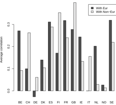
The correlations of housing returns give the first, static, view on the degree of integration of European property markets. We report in Figure 3a the average correlations of European housing markets with their respective 12 (N − 1) counterparts and compare them within the same figure with the average correlations of European housing markets with the 5 non-European countries available in our dataset (AU, CA, JP, NZ and US). It is apparent that the average correlations of European housing markets are not much larger within Europe than with the 5 European countries. Actually, the correlations are even larger with non-European countries for Switzerland, Germany, Finland, United Kingdom and Italy.
INSERT FIGURE 3 HERE
The average correlations are just aggregations of the bilateral correlation measures. To inves-tigate the significance of pairwise correlations further, we report in Figure 3b the proportion of significant pairwise correlations (within Europe and with non-European countries, re-spectively). It emerges that the correlations are not more significant within Europe than with non-European countries. These results show that national European housing markets do not respond more intensively to European global factors than to non-European global factors over the period 1971-2017. This suggests good potential for geographic diversification of investments in European housing markets.
Again, this is a static measure, and our point is precisely to determine whether this has changed over recent years or decades. In addition, a low correlation might reflect the low integration of European housing markets but might also reflect different sensitivities to the global factors. We thus now turn to our multi-factor approach.
4
Results
We first present the profile of the global factors, the weight of the respective real estate mar-kets and the time-varying contribution of the factors to the total variance of our data. We then consider the time-varying explanatory power of the global factors in housing return regres-sions. We also discuss the sensitivity of the results to parameters’ changes (the number of factors and lags and the size of the rolling window). We finally discuss our aggregate mea-sure and study the national level by looking at the country-specific evolution of the adjusted R2, with the aim of assessing better the representativeness of the aggregate R2 measure.
4.1
Global factors
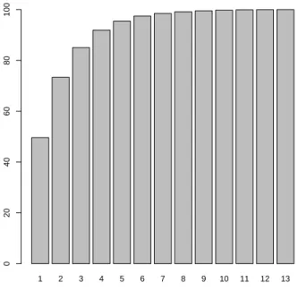
The contributions of the global factors to explaining the total variance of housing returns are summarized in Figure 4a, which reports the cumulative ordered eigenvalues, as derived from the correlation matrix of the 13 series and averaged over the 160 rolling windows. We see that the main factor explains nearly 50% of the total variance, the main 3 factors accounting for more than 80% and 4 factors for 90%.
INSERT FIGURE 4 HERE
While Figure 4a reports the average contribution of the factors over time (the average eigen-value over the 160 rolling windows), Figure 4b shows the evolution of the respective factors’ contributions over time. The figure shows that their contribution is relatively stable, with a big shift around 2008, when the contribution of the first factor rises substantially, which is consistent with the general finding of rising correlations on the financial markets during the crisis.
The apparently low degree of integration resulting from visualization of the graphs6 is
cor-roborated by the Kaiser, Meyer and Olkin (KMO) measure of sampling adequacy, which measures the proportion of variance among variables that might be attributed to common variance. With a measure of sampling adequacy of 0.64 for the full sample, the degree of integration is considered to be low (which confirms the relevance of international diversifi-cation to the full sample).
We finally look at the eigenvectors to identify the contributions of the housing returns to the construction of the global factors. We can see from Figure 5 that the first factor is close to the average of the respective annual returns, as all the elements of the first eigenvector have the same sign (except for Germany, which is precisely the sole country with negative price evolution over the period 1971-2017). Quite interestingly, we notice for the second factor a regional logic with a positive sign for most northern countries (SE, NO, GB, FI, CH) and a negative one for the others.
6The relative eigenvalue of the first principal component below 50% is quite low compared with what is found for equity markets, for which it is closer to 60% (Pukthuanthong and Roll (2009))
INSERT FIGURE 5 HERE
4.2
Explanatory power of linear multi-factor models
These factors are now injected as explanatory variables into the model set out in Equation 3 for explaining annual percentage variations of housing price series. The benchmark model thus includes one set of 3 factors (k = 3) and one set of 3 lagged factors and is based on rolling windows of 6 years (24 quarters). This benchmark model is thus estimated 161 times (184 quarters minus 23 initialization quarters for the rolling window). We report in Figure 6 the evolution of the explanatory power of this model, that is, the adjusted R2, over these 161 quarters (1977-2017). This metrics, which we use as a proxy for the degree of integration, is characterized by 3 periods. First, a quite substantial fall of the R2 occurs around 1981, at the time of the global monetary tightening, with very heterogeneous country dynamics, followed by a relative rise in integration. Second, there is a period of stable but declining integration from 1992 to 2006. Finally, a large increase in the R2 occurs at the time of the 2007-2008 financial crisis, capturing the simultaneous slowdown and, for some markets, the collapse of housing markets, with subsequent normalization returning close to the pre-crisis levels. This first result does not support the view of rising integration but rather suggests a temporary peak of integration related to the 2008 crisis.
INSERT FIGURE 6 HERE
To check whether the crisis was really at the heart of this short-lived rise, we explore some variants of this model by adjusting the size of the rolling window. We can see in Figure 6 that the larger the size of the window (8 years and 10 years compared with the benchmark 6 years), the slower the adjustment to the pre-crisis level. This clearly supports the hypothesis that the 2008-2009 crisis was behind the rise in integration. This result confirms the find-ings of Joyeux and Milunovich (2015), who noted that "Interestingly, all of the convergence intervals coincide either with periods of crisis, or with periods of market exuberance. For instance, evidence of convergence is found during the 2000 dot-com crash, the 2007-2009 subprime crisis and the 2010-2013 European sovereign debt crisis, as well as over the bubble period of 2004-2005."
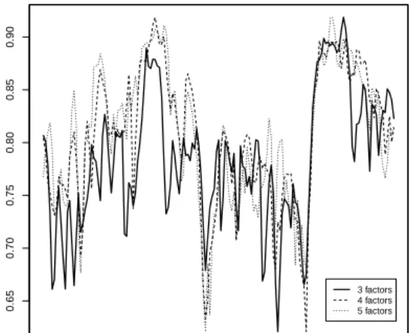
To investigate these results further, we test additional variants by adjusting the number of factors (benchmark three versus four and five factors) to account for a potentially higher number of global sources of variation and by comparing models with factors lagged twice (6 months) or three times (9 months) or with no lag at all to explore the potential time delay in the propagation of global shocks in the system. We find that the profile of the constructed R2 time series is barely affected. We also note that adding one or two sets of lags shifts the
measure of integration upwards, quite logically, though not for the full time window.
4.3
Country specific analysis
The profile of the R2s in Figure 6 is an average of the R2s obtained for the 13 countries of our sample. We now look through the average to establish whether the results that we obtain at the aggregate level represents well what we obtain at the country level.
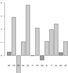
To test whether integration is on the rise or stable at the country level, we regress the R2 for each country on a linear trend during the years of data availability. We observe in Figure 9 that the R2 has an upward trend in most countries (except for Germany and the United
Kingdom) and that this trend is positive and significant at the 5% level in 8 countries (out of 13).
INSERT FIGURE 9 HERE
5
Extensions
We address two key complementary questions, related firstly to the comparison of the in-tegration of European real estate markets with non-European markets and secondly to the emergence of potential regional dynamics via a cluster analysis. We finally discuss some additional robustness checks (based on quarterly variations instead of yearly variations and on ARMA filtering).
5.1
European versus non-European integration
We saw in the preceding section the profile of the integration of European real estate markets over time. One motivation of the paper was to check whether European structural changes (the single market, the monetary union and post-crisis coordination of macroprudential poli-cies) could be captured in the integration measures. However, the changes in our integration measure profile might also be driven by global non-European factors. We thus carry out a comparative analysis to assess whether the integration within Europe just reflects the world dynamics that we also find with non-European countries, in other words to test whether integration within European countries has increased more than with non-European ones. We thus reiterate our estimations by regressing European property returns on global
fac-tors, which are now obtained from our correlation matrix of non-European property returns. Global factors are now interpreted as non-European factors, while the global factors in the preceding sections were "only" capturing commonality at the European level.
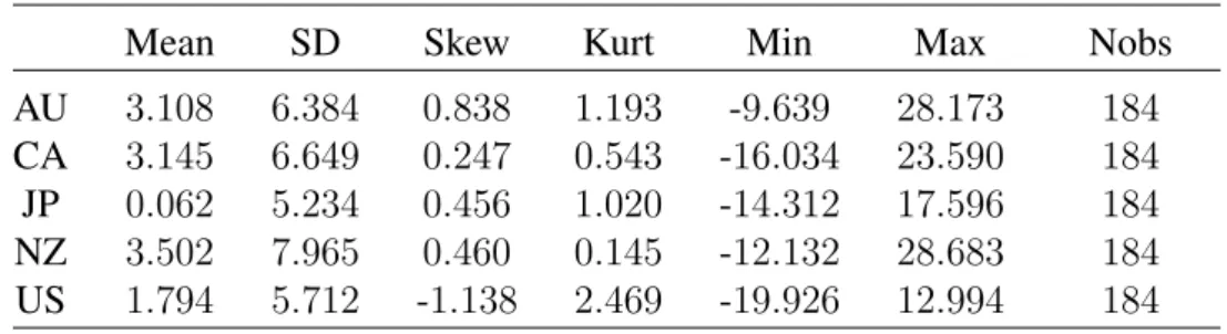
The evolution of the property returns series is reported in Figure 10 and descriptive statistics in Table 2. We see in these 47 years some isolated collapses in 1975 for New Zealand, 1982 for Australia, 1993 for Japan and 2008 for the US, with an apparent common upward trend in the last decade.
INSERT TABLE 2 AND FIGURE 10 HERE
The profile over time of the eigenvalues from the correlation matrix of non-European prop-erty returns is quite different from the one obtained for European countries. Figure 11 shows that the weight of the first factor declines moderately up to 1998, from 60% to 40%, then rises abruptly to nearly 80% and finally returns to 60% (see Figure 10). Remarkably, we find that Japan and New Zealand follow their own dynamics (with more inertia), while the United States, Canada and, to a lesser extent, Australia follow their own, with falls in 1982, 1991 and 2008.
INSERT FIGURE 11 HERE
Quite interestingly, we see that the explanatory power of global factors has a very similar profile, regardless of how we estimate the factors (European versus non-European ones, as illustrated in Figure 12). The integration seems to decline from the 1980s until the 2008 crisis. The subprime crisis then strikes, as we see a sharp increase in integration from 2008 onwards. We finally see a progressive reversal of integration during the last decade. This comparative subsection does not support the hypothesis of a rising integration that is spe-cific to the European level. The European diversification of real estate investments is still effective, no less than the international diversification.
INSERT FIGURE 12 HERE
Looking at the country level, and providing a nuance to our conclusions at the aggregate level, we see some differences in the country-specific time-varying degree of integration. Indeed, only 5 of our 13 European housing return series have a significantly rising R2. This contrasts with the findings obtained from our analysis based on European global factors, in which 8 of the 13 series show a significantly positive increase in integration.
INSERT FIGURE 13 HERE
5.2
Regional integration
European housing markets are quite heterogeneous and we do not expect countries as distant as Spain and Finland to be closely integrated. Since the bottom line so far is that we do not find in the data significantly rising integration at the European level (only temporarily around the 2008 crisis), and it is not stronger than integration with non-European countries, we examine in this extension whether integration would emerge at the regional level. We thus rely on a clustering methodology (the K-means clustering algorithm), which groups countries according to the similarity of their beta exposures to the global factors. Based on standard tools for k-determination (the Elbow method minimizing the total intra-cluster
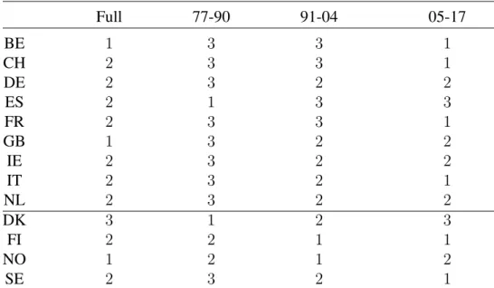
variation - or the within-cluster sum of squares - and the Silhouette method maximizing the average silhouette coefficient; Kaufman and Rousseeuw (1990)), we identify up to three clusters (three according to the Elbow method and two according to the Silhouette method). We report in Figure 14 a map of Europe with colours corresponding to these three respective clusters. We also investigate the stability over time of the clusters (see Table 3). We find that the clusters are not stable over time. We also isolate the Nordic countries (Denmark, Finland, Norway and Sweden) in Table 3 to determine whether they are characterized by some regional commonality, without success. The data do not support regional integration. European diversification also matters at the regional level.
INSERT FIGURE 14 AND TABLE 3 HERE
5.3
Robustness complements
5.3.1 Quarterly and yearly variations
We reiterate this analysis by working with quarterly variations instead of yearly variations. The rationale behind our choice of annual variations is first to fix potential seasonality is-sues and then to enhance the capture of co-movement by allowing up to three quarters of delay between responses to shocks. Of course, the choice to work with annual variations of quarterly prices also artificially brings some autocorrelation into the data and thus noise into the regressions. To check whether this choice has an impact on our results, we reiterate the analysis with quarterly data and it turns out that the choice has barely any effect on the analysis outcomes.
5.3.2 ARMA filtering
Since the main input in principal component analysis is the covariance of our time series, the first key check is to make sure that the covariance is stationary. The annual returns that we use in this work are clearly stationary according to the standard stationary tests. We proceed further in this section and filter the autocorrelation of our returns with the aim of making the series iid. The benefit of filtering the dynamics of the series is to improve the identification of the global factors. The downside is that the filter at the same time removes an autocorrelation that partially captures the effect of slowly propagating global factor shocks. Again, we investigate the effect on our results of ARMA filtering and find that the results remain barely unchanged, which suggests that the inclusion of lagged factors is enough to capture the delayed effects of global factors.
6
Conclusions
The 2007-2008 financial crisis has given rise to a general increase in the correlations of macro-financial indicators. Some investors had to cope with a sudden loss of diversification power in their portfolios. Housing markets were no different. The correlations increased considerably around 2008.
The question is whether this rise was short-lived or whether something more fundamental changed in the real estate markets. Indeed, since 1999, the euro has been adopted as a common currency in many countries (19 countries in 2019). In addition, since 2010, the European Systemic Risk Board, has made common coordinated recommendations to most European countries (28 countries in 2019) on real estate market stability, among others. Whether this higher regulatory integration gives rise to stronger economic integration was the subject of our investigation.
We rely on the time-varying explanatory power of a linear multi-factor model to assess the degree of integration of the European housing markets. We find that the rise in integration subsequent to the 2007-2008 crisis was short-lived and that the average degree of integration returns to a level that, while marginally higher, is similar to the pre-crisis one, despite a significant rise in integration in 8 of our 13 European countries over the period 1971 to 2017. We compare the degree of within-Europe integration with the degree of integration of European countries with the rest of the world and find that the time-varying profiles of integration are very similar, supporting the view that no recent change is specific to the European integration dynamics. We also find that real estate markets are not integrated at the regional level.
Our results matter for investment strategies in the housing market and show that the loss of diversification power, that is, the rising integration, around 2008 was short-lived and associ-ated with the financial crisis. These results are in line with those of Joyeux and Milunovich (2015), who noted: "Interestingly, all of the convergence intervals coincide either with peri-ods of crisis, or with periperi-ods of market exuberance." Although smaller during crisis episodes, the geographic diversification of real estate investments in European markets still matters. This paper could be extended in several directions. First, we could work on country
res-idential price series. More granular data isolating urban from rural areas would probably show different dynamics. Similarly, commercial real estate has different, and probably more integrated, dynamics that would also deserve a specific analysis. Second, the evolution of integration is informative regarding diversification benefits, but this has not been specifically tested in this paper and has not been related to rebalancing strategies. This is certainly a promising next step. Third, the section devoted to regional clustering could be extended by considering spatial dependences based on distance or on common borders.
References
Billio, M., Donadelli, M., Paradiso, A., and Riedel, M. (2017). Which market integration measure? Journal of Banking & Finance, 76(C):150–174.
Bond, S. A., Karolyi, G. A., and Sanders, A. B. (2003). International Real Estate Returns: A Multifactor, Multicountry Approach. Real Estate Economics, 31:481–500.
Case, B., Goetzmann, W. N., and Rouwenhorst, K. G. (2000). Global Real Estate Markets - Cycles and Fundamentals. NBER Working Papers 7566, National Bureau of Economic Research, Inc.
Christoffersen, P., Lunde, A., and Olesen, K. V. (2019). Factor structure in commodity futures return and volatility. Journal of Financial and Quantitative Analysis, 54(3):1083– 1115.
Cotter, J., Gabriel, S., and Roll, R. (2015). Can Housing Risk Be Diversified? A Cautionary Tale from the Housing Boom and Bust. Review of Financial Studies, 28(3):913–936.
de Wit, I. (2010). International diversification strategies for direct real estate. Journal of Real Estate Finance and Economics, 41(4):433–457.
Druica, E., Valsan, C., and Ianole, R. (2015). Residential Real Estate in Europe: An Explo-ration of Common Risk Factors. Review of Economic Perspectives, 15(4):413–429.
Eichholtz, P. M. (1996). Does international diversification work better for real estate than for stocks and bonds? Financial Analysts Journal, 52(1):56–62.
Gallo, J. G., Lockwood, L. J., and Zhang, Y. (2013). Structuring Global Property Portfolios: A Cointegration Approach. Journal of Real Estate Research, 35(1):53–82.
Jeffrey, R. F., Barkbu, B., Blavy, R., Oman, W., and Schoelermann, H. (2018). Economic convergence in the euro area: Coming together or drifting apart? Working Paper 18/10, IMF.
Joyeux, R. and Milunovich, G. (2015). Speculative bubbles, financial crises and convergence in global real estate investment trusts. Applied Economics, 47(27):2878–2898.
Kaufman, L. and Rousseeuw, P. (1990). Finding Groups in Data: an introduction to cluster analysis. Wiley.
Lee, S. (2005). The Return due to Diversification of Real Estate to the US Mixed-Asset Portfolio. Journal of Real Estate Portfolio Management, 11(1):19–28.
Lee, S. (2009). Is The Uk Real Estate Market Converging With The Rest Of Europe? Journal of European Real Estate Research, 2(1).
Lee, S. (2010). Are the Returns of the Spanish Real Estate Market Converging with the Rest of Europe? Unpublished.
McAllister, P. (2001). Convergence in European Real Estate Markets: Theoretical Perspec-tives and Empirical Evidence. ERES eres2001-225, European Real Estate Society (ERES).
Pukthuanthong, K. and Roll, R. (2009). Global market integration: An alternative measure and its application. Journal of Financial Economics, 94(2):214–232.
Scatigna, M., Szemere, R., and Tsatsaronis, K. (2014). Residential property price statistics across the globe. BIS Quarterly Review.
Srivatsa, R. and Lee, S. (2010). European Real Estate Markets Convergence. ERES eres2010-097, European Real Estate Society (ERES).
Tables and Figures
Table 1: Descriptive statistics of real estate annual returns - Europe - 1972-2017
Mean SD Skew Kurt Min Max Nobs BE 2.360 5.151 -0.803 1.168 -13.414 12.747 184 CH 1.094 4.922 -0.261 0.254 -10.841 15.620 184 DE -0.082 2.510 0.440 -0.422 -4.901 6.040 184 DK 1.908 8.588 0.131 0.242 -17.675 27.933 184 ES 2.733 9.776 0.374 0.123 -18.167 33.185 184 FI 1.842 8.895 0.240 1.626 -21.141 34.094 184 FR 2.142 4.865 0.317 -0.481 -9.022 13.717 184 GB 3.836 9.689 0.513 0.804 -17.762 38.494 184 IE 2.944 9.365 -0.368 -0.068 -21.557 23.726 184 IT 1.786 7.156 1.582 3.465 -9.307 32.541 184 NL 2.706 8.690 0.387 2.215 -21.151 37.519 184 NO 3.374 7.988 -0.157 0.247 -18.115 25.205 184 SE 2.753 6.935 -0.698 0.105 -18.215 14.168 184 Average 2.261 7.271 0.131 0.714 -15.482 24.230 184
Note: BIS real estate long price series, as CPI deflated. Annual percentage variations of quarterly data.
Table 2: Descriptive statistics of real estate annual returns - Non-Europe - 1972-2017
Mean SD Skew Kurt Min Max Nobs AU 3.108 6.384 0.838 1.193 -9.639 28.173 184 CA 3.145 6.649 0.247 0.543 -16.034 23.590 184 JP 0.062 5.234 0.456 1.020 -14.312 17.596 184 NZ 3.502 7.965 0.460 0.145 -12.132 28.683 184 US 1.794 5.712 -1.138 2.469 -19.926 12.994 184
Note: BIS real estate long price series, as CPI deflated. Annual percentage variations of quarterly data.
Table 3: Cluster analysis based on similarity of country exposures to global factors Full 77-90 91-04 05-17 BE 1 3 3 1 CH 2 3 3 1 DE 2 3 2 2 ES 2 1 3 3 FR 2 3 3 1 GB 1 3 2 2 IE 2 3 2 2 IT 2 3 2 1 NL 2 3 2 2 DK 3 1 2 3 FI 2 2 1 1 NO 1 2 1 2 SE 2 3 2 1
Note: Cluster analysis based on K-means algorithm where the partition of the 13 countries in 3 clusters is based on minimizing the within-cluster sum of squares of βs from equation 3. Values 1, 2 and 3 refer to the 3 specific clusters. Values are to be interpreted on a column basis only, as the attribution of values 1, 2 and 3 across the different sub-samples is arbitrary. Last four rows collect figures for the Nordic countries.
50 100 150 200 250 CPI deflated PP 1995=100 BE CH DE DK ES FI FR 1971 1976 1981 1986 1991 1996 2001 2006 2011 2016 50 100 150 200 250 300 350 CPI deflated PP 1995=100 GB IE IT NL NO SE 1971 1976 1981 1986 1991 1996 2001 2006 2011 2016
− 20 − 10 0 10 20 30 CPI deflated PP 1995=100 BE CH DE DK ES FI FR 1972 1977 1982 1987 1992 1997 2002 2007 2012 2017 − 20 − 10 0 10 20 30 40 CPI deflated PP 1995=100 GB IE IT NL NO SE 1972 1977 1982 1987 1992 1997 2002 2007 2012 2017
BE CH DE DK ES FI FR GB IE IT NL NO SE With Eur With Non−Eur A v er age correlation 0.0 0.1 0.2 0.3
(a) Average pairwise correlations of European national real estate return series with series of Eur and non-Eur countries
BE CH DE DK ES FI FR GB IE IT NL NO SE
With Eur With Non−Eur
Propor
tion of significant pairwise correlations
0 20 40 60 80 100
(b) Proportion of significant pairwise correlations real estate return series with series of Eur and non-Eur countries
1 2 3 4 5 6 7 8 9 10 11 12 13 0 20 40 60 80 100
(a) Average cumulative percentage of variance explained by sorted eigenvalues. The cu-mulative percentage of variance is explained within each estimation window of 6 years by spectral decomposition of the correlation matrix of the real estate annual returns. The average is taken over the 160 overlapping rolling windows.
0 20 40 60 80 100 1977 1981 1985 1989 1993 1997 2001 2005 2009 2013 2017
(b) Stacked 5 largest eigenvalues as computed for each time window of 6 years by spectral decomposition of the correlation matrix of the real estate annual returns.
BE CH DE DK ES FI FR GB IE IT NL NO SE Contribution to factor 1 0.0 0.1 0.2 0.3 BE CH DE DK ES FI FR GB IE IT NL NO SE Contribution to factor 2 −0.2 0.0 0.2 0.4 BE CH DE DK ES FI FR GB IE IT NL NO SE Contribution to factor 3 −0.4 0.0 0.2 0.4
Figure 5: Eigenvectors associated to factors 1, 2 and 3. Values thus represent the country coefficients used in the linear combindations of national real estate returns designed to build factors 1, 2 and 3. 0.65 0.70 0.75 0.80 0.85 0.90 6Y (benchm) 8Y 10Y 1981 1985 1989 1993 1997 2001 2005 2009 2013 2017
Figure 6: Indicators of global market integration. Our measure of market integration is the cross-country average of the adjusted R2 from Equation 3. Comparison of the benchmark model (6-years window) with alternative estimation windows (8 and 10 years).
0.65 0.70 0.75 0.80 0.85 0.90 1977 1981 1985 1989 1993 1997 2001 2005 2009 2013 2017 3 factors 4 factors 5 factors
Figure 7: Indicators of global market integration. Our measure of market integration is the cross-country average of the adjusted R2 from Equation 3. Comparison of the benchmark model (3 factors) with alternative number of factors (4 and 5 factors).
0.65 0.70 0.75 0.80 0.85 0.90 1977 1981 1985 1989 1993 1997 2001 2005 2009 2013 2017 1 lag (benchm) No lag 2 lags 3 lags
Figure 8: Indicators of global market integration. Our measure of market integration is the cross-country average of the adjusted R2 from Equation 3. Comparison of the benchmark
BE CH DE DK ES FI FR GB IE IT NL NO SE 0 2 4 6 8
Figure 9: Time trend t-stats for adjusted R2s from global factor models (Equation 3). Light grey if trend significant at 5%.
− 20 − 10 0 10 20 30 CPI deflated PP 1995=100 AU CA JP NZ US 1972 1977 1982 1987 1992 1997 2002 2007 2012 2017
Figure 10: BIS Property Price Indices annual percentage variations of CPI deflated series -Non-European countries
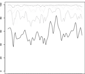
0 20 40 60 80 100 1977 1981 1985 1989 1993 1997 2001 2005 2009 2013 2017
Figure 11: Stacked 5 eigenvalues as computed for each time window of 6 years by spectral decomposition of the correlation matrix of the real estate annual returns - Non-European countries 0.65 0.70 0.75 0.80 0.85 0.90 1977 1981 1985 1989 1993 1997 2001 2005 2009 2013 2017 Eur Non−Eur
Figure 12: Indicators of global market integration. Our measure of market integration is the cross-country average of the adjusted R2 from Equation 3. Comparison of the benchmark model (factors computed from the correlation matrix of European real estate returns) with global factor source (factors computed from the correlation matrix of non-European real estate returns).
BE CH DE DK ES FI FR GB IE IT NL NO SE 0 2 4 6 8
Figure 13: Time trend t-stats for adjusted R2s from global factor models computed from the correlation matrix of Non-European real estate returns. Light grey if trend significant at 5%.
Figure 14: Map of the 3 European regional clusters resulting from the K-means algorithm, as applied on the full sample.