HAL Id: hal-02268468
https://hal.archives-ouvertes.fr/hal-02268468
Submitted on 20 May 2020
HAL is a multi-disciplinary open access
archive for the deposit and dissemination of
sci-entific research documents, whether they are
pub-lished or not. The documents may come from
teaching and research institutions in France or
abroad, or from public or private research centers.
L’archive ouverte pluridisciplinaire HAL, est
destinée au dépôt et à la diffusion de documents
scientifiques de niveau recherche, publiés ou non,
émanant des établissements d’enseignement et de
recherche français ou étrangers, des laboratoires
publics ou privés.
Fast approximation of eccentricities and distances in
hyperbolic graphs
Victor Chepoi, Feodor Dragan, Michel Habib, Yann Vaxès, Hend Alrasheed
To cite this version:
Victor Chepoi, Feodor Dragan, Michel Habib, Yann Vaxès, Hend Alrasheed. Fast approximation of
eccentricities and distances in hyperbolic graphs. Journal of Graph Algorithms and Applications,
Brown University, 2019, 23 (2), pp.393-433. �10.7155/jgaa.00496�. �hal-02268468�
arXiv:1805.07232v1 [cs.DS] 17 May 2018
Fast approximation of centrality and distances in hyperbolic
graphs
Victor Chepoi1, Feodor F. Dragan2, Michel Habib3, Yann Vax`es1, and Hend Al-Rasheed2
1
Laboratoire d’Informatique et Syst`emes, Aix-Marseille Univ, CNRS, and Univ. de Toulon
Facult´e des Sciences de Luminy, F-13288 Marseille Cedex 9, France {victor.chepoi, yann.vaxes}@lif.univ-mrs.fr
2
Algorithmic Research Laboratory, Department of Computer Science, Kent State University, Kent, Ohio, USA
[email protected], [email protected]
3
Institut de Recherche en Informatique Fondamentale, University Paris Diderot - Paris7, F-75205 Paris Cedex 13, France
Abstract. We show that the eccentricities (and thus the centrality indices) of all vertices of a
δ-hyperbolic graph G = (V, E) can be computed in linear time with an additive one-sided error of at most cδ, i.e., after a linear time preprocessing, for every vertex v of G one can compute in O(1) time an estimate ˆe(v) of its eccentricity eccG(v) such that eccG(v) ≤ ˆe(v) ≤ eccG(v) + cδ for a small constant
c. We prove that every δ-hyperbolic graph G has a shortest path tree, constructible in linear time, such that for every vertex v of G, eccG(v) ≤ eccT(v) ≤ eccG(v) + cδ. These results are based on an
interesting monotonicity property of the eccentricity function of hyperbolic graphs: the closer a vertex is to the center of G, the smaller its eccentricity is. We also show that the distance matrix of G with an additive one-sided error of at most c′δcan be computed in O(|V |2
log2
|V |) time, where c′< cis a small
constant. Recent empirical studies show that many real-world graphs (including Internet application networks, web networks, collaboration networks, social networks, biological networks, and others) have small hyperbolicity. So, we analyze the performance of our algorithms for approximating centrality and distance matrix on a number of real-world networks. Our experimental results show that the obtained estimates are even better than the theoretical bounds.
1
Introduction
The diameter diam(G) and the radius rad(G) of a graph G = (V, E) are two fundamental metric parameters that have many important practical applications in real world networks. The problem of finding the center
C(G) of a graph G is often studied as a facility location problem for networks where one needs to select a
single vertex to place a facility so that the maximum distance from any demand vertex in the network is minimized. In the analysis of social networks (e.g., citation networks or recommendation networks), biological systems (e.g., protein interaction networks), computer networks (e.g., the Internet or peer-to-peer networks), transportation networks (e.g., public transportation or road networks), etc., the eccentricity ecc(v) of a vertex
v is used to measure the importance of v in the network: the centrality index of v [69] is defined as ecc(v)1 . Being able to compute efficiently the diameter, center, radius, and vertex centralities of a given graph has become an increasingly important problem in the analysis of large networks. The algorithmic complexity of the diameter and radius problems is very well-studied. For some special classes of graphs there are efficient algorithms [8,18,25,30,33,38,42,53,56,62,79]. However, for general graphs, the only known algorithms computing the diameter and the radius exactly compute the distance between every pair of vertices in the graph, thus solving the all-pairs shortest paths problem (APSP) and hence computing all eccentricities. In view of recent negative results [8,21,83], this seems to be the best what one can do since even for graphs with
m = O(n) (where m is the number of edges and n is the number of vertices) the existence of a subquadratic
time (that is, O(n2−ǫ) time for some ǫ > 0) algorithm for the diameter or the radius problem will refute the
well known Strong Exponential Time Hypothesis (SETH). Furthermore, recent work [9] shows that if the radius of a possibly dense graph (m = O(n2)) can be computed in subcubic time (O(n3−ǫ) for some ǫ > 0),
then APSP also admits a subcubic algorithm. Such an algorithm for APSP has long eluded researchers, and it is often conjectured that it does not exist (see, e.g., [84,90]).
Motivated by these negative results, researches started devoting more attention to development of fast approximation algorithms. In the analysis of large-scale networks, for fast estimations of diameter, center, radius, and centrality indices, linear or almost linear time algorithms are desirable. One hopes also for the all-pairs shortest paths problem to have o(nm) time small-constant–factor approximation algorithms. In general graphs, both diameter and radius can be 2-approximated by a simple linear time algorithm which picks any node and reports its eccentricity. A 3/2-approximation algorithm for the diameter and the radius which runs in ˜O(mn2/3)1 time was recently obtained in [31] (see also [12] for an earlier ˜O(n2 + m√n)
time algorithm and [83] for a randomized ˜O(m√n) time algorithm). For the sparse graphs, this is an o(n2)
time approximation algorithm. Furthermore, under plausible assumptions, no O(n2−ǫ) time algorithm can
exist that (3/2 − ǫ′)-approximates (for ǫ, ǫ′ > 0) the diameter [83] and the radius [8] in sparse graphs.
Similar results are known also for all eccentricities: a 5/3-approximation to the eccentricities of all vertices can be computed in ˜O(m3/2) time [31] and, under plausible assumptions, no O(n2−ǫ) time algorithm can
exist that (5/3 − ǫ′)-approximates (for ǫ, ǫ′ > 0) the eccentricities of all vertices in sparse graphs [8]. Better
approximation algorithms are known for some special classes of graphs [27,34,35,42,43,50,51,54,94]. A number of heuristics for approximating diameters, radii and eccentricities in real-world graphs were proposed and investigated in [10,21,22,23,69,24,52].
Approximability of APSP is also extensively investigated. An additive 2-approximation for APSP in unweighted undirected graphs (the graphs we consider in this paper) was presented in [46]. It runs in
˜
O(min{n3/2m1/2, n7/3}) time and hence improves the runtime of an earlier algorithm from [12]. In [19], an
˜
O(n2) time algorithm was designed which computes an approximation of all distances with a multiplicative
error of 2 and an additive error of 1. Furthermore, [19] gives an O(n2.24+o(1)ǫ−3log(n/ǫ)) time algorithm
that computes an approximation of all distances with a multiplicative error of (1 + ǫ) and an additive error of 2. The latter improves an earlier algorithm from [58]. Better algorithms are known for some special classes of graphs (see [25,35,49,89] and papers cited therein).
The need for fast approximation algorithms for estimating diameters, radii, centrality indices, or all pairs shortest paths in large-scale complex networks dictates to look for geometric and topological properties of those networks and utilize them algorithmically. The classical relationships between the diameter, radius, and center of trees and folklore linear time algorithms for their computation is one of the departing points of this research. A result from 1869 by C. Jordan [66] asserts that the radius of a tree T is roughly equal to half of its diameter and the center is either the middle vertex or the middle edge of any diametral path. The diameter and a diametral pair of T can be computed (in linear time) by a simple but elegant procedure: pick any vertex x, find any vertex y furthest from x, and find once more a vertex z furthest from y; then return {y, z} as a diametral pair. One computation of a furthest vertex is called an FP scan; hence the diameter of a tree can be computed via two FP scans. This two FP scans procedure can be extended to exact or approximate computation of the diameter and radius in many classes of tree-like graphs. For example, this approach was used to compute the radius and a central vertex of a chordal graph in linear time [33]. In this case, the center of G is still close to the middle of all (y, z)-shortest paths and dG(y, z) is not the diameter but
is still its good approximation: d(y, z) ≥ diam(G) − 2. Even better, the diameter of any chordal graph can be approximated in linear time with an additive error 1 [54]. But it turns out that the exact computation of diameters of chordal graphs is as difficult as the general diameter problem: it is even difficult to decide if the diameter of a split graph is 2 or 3.
The experience with chordal graphs shows that one have to abandon the hope of having fast exact algorithms, even for very simple (from metric point of view) graph-classes, and to search for fast algorithms approximating diam(G), rad(G), C(G), eccG(v) with a small additive constant depending only of the coarse
geometry of the graph. Gromov hyperbolicity or the negative curvature of a graph (and, more generally, of a metric space) is one such constant. A graph G = (V, E) is δ-hyperbolic [14,59,28,60] if for any four vertices
w, v, x, y of G, the two largest of the three distance sums d(w, v) + d(x, y), d(w, x) + d(v, y), d(w, y) + d(v, x)
differ by at most 2δ ≥ 0. The hyperbolicity δ(G) of a graph G is the smallest number δ such that G is
δ-hyperbolic. The hyperbolicity can be viewed as a local measure of how close a graph is metrically to a tree:
1 ˜
the smaller the hyperbolicity is, the closer its metric is to a tree-metric (trees are 0-hyperbolic and chordal graphs are 1-hyperbolic).
Recent empirical studies showed that many real-world graphs (including Internet application networks, web networks, collaboration networks, social networks, biological networks, and others) are tree-like from a metric point of view [10,11,20] or have small hyperbolicity [67,77,85]. It has been suggested in [77], and recently formally proved in [39], that the property, observed in real-world networks, in which traffic between nodes tends to go through a relatively small core of the network, as if the shortest paths between them are curved inwards, is due to the hyperbolicity of the network. Bending property of the eccentricity function in hyperbolic graphs were used in [16,15] to identify core-periphery structures in biological networks. Small hyperbolicity in real-world graphs provides also many algorithmic advantages. Efficient approximate solutions are attainable for a number of optimization problems [35,36,37,39,40,44,57,92].
In [35] we initiated the investigation of diameter, center, and radius problems for δ-hyperbolic graphs and we showed that the existing approach for trees can be extended to this general framework. Namely, it is shown in [35] that if G is a δ-hyperbolic graph and {y, z} is the pair returned after two FP scans, then
d(y, z) ≥ diam(G) − 2δ, diam(G) ≥ 2rad(G) − 4δ − 1, diam(C(G)) ≤ 4δ + 1, and C(G) is contained in
a small ball centered at a middle vertex of any shortest (y, z)-path. Consequently, we obtained linear time algorithms for the diameter and radius problems with additive errors linearly depending on the input graph’s hyperbolicity.
In this paper, we advance this line of research and provide a linear time algorithm for approximate computation of the eccentricities (and thus of centrality indices) of all vertices of a δ-hyperbolic graph G, i.e., we compute the approximate values of all eccentricities within the same time bounds as one computes the approximation of the largest or the smallest eccentricity (diam(G) or rad(G)). Namely, the algorithm outputs for every vertex v of G an estimate ˆe(v) of eccG(v) such that eccG(v) ≤ ˆe(v) ≤ eccG(v) + cδ, where
c > 0 is a small constant. In fact, we demonstrate that G has a shortest path tree, constructible in linear time,
such that for every vertex v of G, eccG(v) ≤ eccT(v) ≤ eccG(v)+cδ (a so-called eccentricity cδ-approximating
spanning tree). This is our first main result of this paper and the main ingredient in proving it is the following
interesting dependency between the eccentricities of vertices of G and their distances to the center C(G): up to an additive error linearly depending on δ, eccG(v) is equal to d(v, C(G)) plus rad(G). To establish
this new result, we have to revisit the results of [35] about diameters, radii, and centers, by simplifying their proofs and extending them to all eccentricities.
Eccentricity k-approximating spanning trees were introduced by Prisner in [81]. A spanning tree T of a graph G is called an eccentricity k-approximating spanning tree if for every vertex v of G eccT(v) ≤ eccG(v)+k
holds [81]. Prisner observed that any graph admitting an additive tree k-spanner (that is, a spanning tree T such that dT(v, u) ≤ dG(v, u) + k for every pair u, v) admits also an eccentricity k-approximating spanning
tree. Therefore, eccentricity k-approximating spanning trees exist in interval graphs for k = 2 [70,75,80], in asteroidal-triple–free graph [70], strongly chordal graphs [26] and dually chordal graphs [26] for k = 3. On the other hand, although for every k there is a chordal graph without an additive tree k-spanner [70,80], yet as Prisner demonstrated in [81], every chordal graph has an eccentricity 2-approximating spanning tree. Later this result was extended in [51] to a larger family of graphs which includes all chordal graphs and all plane triangulations with inner vertices of degree at least 7. Both those classes belong to the class of 1-hyperbolic graphs. Thus, our result extends the result of [81] to all δ-hyperbolic graphs.
As our second main result, we show that in every δ-hyperbolic graph G all distances with an addi-tive one-sided error of at most c′δ can be found in O(|V |2log2|V |) time, where c′ < c is a small
con-stant. With a recent result in [32], this demonstrates an equivalence between approximating the hyperbol-icity and approximating the distances in graphs. Note that every δ-hyperbolic graph G admits a distance approximating tree T [35,36,37], that is, a tree T (which is not necessarily a spanning tree) such that
dT(v, u) ≤ dG(v, u) + O(δ log n) for every pair u, v. Such a tree can be used to compute all distances in G
with an additive one-sided error of at most O(δ log n) in O(|V |2) time. Our new result removes the
depen-dency of the additive error from log n and has a much smaller constant in front of δ. Note also that the tree T may use edges not present in G (not a spanning tree of G) and thus cannot serve as an eccentricity
O(δ log n)-approximating spanning tree. Furthermore, as chordal graphs are 1-hyperbolic, for every k there
At the conclusion of this paper, we analyze the performance of our algorithms for approximating eccen-tricities and distances on a number of real-world networks. Our experimental results show that the estimates on eccentricities and distances obtained are even better than the theoretical bounds proved.
2
Preliminaries
2.1 Center, diameter, centrality
All graphs G = (V, E) occurring in this paper are finite, undirected, connected, without loops or multiple edges. We use n and |V | interchangeably to denote the number of vertices and m and |E| to denote the number of edges in G. The length of a path from a vertex v to a vertex u is the number of edges in the path. The distance dG(u, v) between vertices u and v is the length of a shortest path connecting u and v
in G. The eccentricity of a vertex v, denoted by eccG(v), is the largest distance from v to any other vertex,
i.e., eccG(v) = maxu∈V dG(v, u). The centrality index of v is eccG1(v). The radius rad(G) of a graph G is
the minimum eccentricity of a vertex in G, i.e., rad(G) = minv∈V eccG(v). The diameter diam(G) of a
graph G is the the maximum eccentricity of a vertex in G, i.e., diam(G) = maxv∈V eccG(v). The center
C(G) = {c ∈ V : eccG(c) = rad(G)} of a graph G is the set of vertices with minimum eccentricity. 2.2 Gromov hyperbolicity and thin geodesic triangles
Let (X, d) be a metric space. The Gromov product of y, z ∈ X with respect to w is defined to be (y|z)w=
1
2(d(y, w) + d(z, w) − d(y, z)). A metric space (X, d) is said to be δ-hyperbolic [60] for δ ≥ 0 if
(x|y)w≥ min{(x|z)w, (y|z)w} − δ
for all w, x, y, z ∈ X. Equivalently, (X, d) is δ-hyperbolic if for any four points u, v, x, y of X, the two largest of the three distance sums d(u, v) + d(x, y), d(u, x) + d(v, y), d(u, y) + d(v, x) differ by at most 2δ ≥ 0. A connected graph G = (V, E) is δ-hyperbolic (or of hyperbolicity δ) if the metric space (V, dG) is δ-hyperbolic,
where dG is the standard shortest path metric defined on G.
δ-Hyperbolic graphs generalize k-chordal graphs and graphs of bounded tree-length: each k-chordal graph
has the tree-length at most ⌊k2⌋ [47] and each tree-length λ graph has hyperbolicity at most λ [35,36]. Recall
that a graph is k-chordal if its induced cycles are of length at most k, and it is of tree-length λ if it has a Robertson-Seymour tree-decomposition into bags of diameter at most λ [47].
For geodesic metric spaces and graphs there exist several equivalent definitions of δ-hyperbolicity involving different but comparable values of δ [14,28,59,60]. In this paper, we will use the definition via thin geodesic
triangles. Let (X, d) be a metric space. A geodesic joining two points x and y from X is a (continuous)
map f from the segment [a, b] of R1 of length |a − b| = d(x, y) to X such that f(a) = x, f(b) = y, and d(f (s), f (t)) = |s − t| for all s, t ∈ [a, b]. A metric space (X, d) is geodesic if every pair of points in X can
be joined by a geodesic. Every unweighted graph G = (V, E) equipped with its standard distance dG can be
transformed into a geodesic (network-like) space (X, d) by replacing every edge e = uv by a segment [u, v] of length 1; the segments may intersect only at common ends. Then (V, dG) is isometrically embedded in a
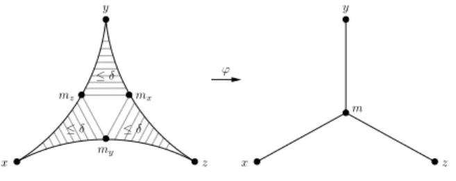
natural way in (X, d). The restrictions of geodesics of X to the vertices V of G are the shortest paths of G. Let (X, d) be a geodesic metric space. A geodesic triangle ∆(x, y, z) with x, y, z ∈ X is the union [x, y] ∪ [x, z]∪[y, z] of three geodesic segments connecting these vertices. Let mxbe the point of the geodesic segment
[y, z] located at distance αy:= (x|z)y = (d(y, x) + d(y, z) − d(x, z))/2 from y. Then mxis located at distance
αz := (y|x)z = (d(z, y) + d(z, x) − d(y, x))/2 from z because αy + αz = d(y, z). Analogously, define the
points my ∈ [x, z] and mz ∈ [x, y] both located at distance αx := (y|z)x = (d(x, y) + d(x, z) − d(y, z))/2
from x; see Fig. 1 for an illustration. There exists a unique isometry ϕ which maps ∆(x, y, z) to a tripod
T (x, y, z) consisting of three solid segments [x, m], [y, m], and [z, m] of lengths αx, αy, and αz, respectively.
mx, my, and mz to the center m of this tripod. Any other point of T (x, y, z) is the image of exactly two
points of ∆(x, y, z). A geodesic triangle ∆(x, y, z) is called δ-thin if for all points u, v ∈ ∆(x, y, z), ϕ(u) = ϕ(v) implies d(u, v) ≤ δ. A graph G = (V, E) whose all geodesic triangles ∆(u, v, w), u, v, w ∈ V , are δ-thin is called a graph with δ-thin triangles, and δ is called the thinness parameter of G.
x y z x y z mz my m ϕ mx ≤δ ≤δ ≤δ
Fig. 1. A geodesic triangle ∆(x, y, z), the points mx, my, mz, and the tripod Υ (x, y, z)
The following result shows that hyperbolicity of a geodesic space or a graph is equivalent to having thin geodesic triangles.
Proposition 1 ([14,28,59,60]). Geodesic triangles of geodesic δ-hyperbolic spaces or graphs are 4δ-thin.
Conversely, geodesic spaces or graphs with δ-thin triangles are δ-hyperbolic.
In what follows, we will need few more notions and notations. Let G = (V, E) be a graph. By [x, y] we denote a shortest path connecting vertices x and y in G; we call [x, y] a geodesic between x and y. A ball B(s, r) of G centered at vertex s ∈ V and with radius r is the set of all vertices with distance no more than r from
s (i.e., B(s, r) := {v ∈ V : dG(v, s) ≤ r}). The kth-power of a graph G = (V, E) is the graph Gk = (V, E′)
such that xy ∈ E′ if and only if 0 < d
G(x, y) ≤ k. Denote by F (x) := {y ∈ V : dG(x, y) = eccG(x)} the set of
all vertices of G that are most distant from x. Vertices x and y of G are called mutually distant if x ∈ F (y) and y ∈ F (x), i.e., eccG(x) = eccG(y) = dG(x, y).
3
Fast approximation of eccentricities
In this section, we give linear and almost linear time algorithms for sharp estimation of the diameters, the radii, the centers and the eccentricities of all vertices in graphs with δ-thin triangles. Before presenting those algorithms, we establish some conditional lower bounds on complexities of computing the diameters and the radii in those graphs.
3.1 Conditional lower bounds on complexities
Recent work has revealed convincing evidence that solving the diameter problem in subquadratic time might not be possible, even in very special classes of graphs. Roditty and Vassilevska W. [83] showed that an algorithm that can distinguish between diameter 2 and 3 in a sparse graph in subquadratic time refutes the following widely believed conjecture.
The Orthogonal Vectors Conjecture: There is no ǫ > 0 such that for all c ≥ 1, there is an algorithm that
given two lists of n binary vectors A, B ⊆ {0, 1}d where d = c log n can determine if there is an orthogonal
pair a ∈ A, b ∈ B, in O(n2−e) time.
Williams [95] showed that the Orthogonal Vectors (OV) Conjecture is implied by the well-known Strong Exponential Time Hypothesis (SETH) of Impagliazzo, Paturi, and Zane [64,63]. Nowadays many papers base the hardness of problems on SETH and the OV conjecture (see, e.g., [8,21,91] and papers cited therein).
Since all geodesic triangles of a graph constructed in the reduction in [83] are 2-thin, we can rephrase the result from [83] as follows.
Statement 1 If for some ǫ > 0, there is an algorithm that can determine if a given graph with 2-thin
triangles, n vertices and m = O(n) edges has diameter 2 or 3 in O(n2−ǫ) time, then the Orthogonal Vector Conjecture is false.
To prove a similar lower bound result for the radius problem, recently Abboud et al. [8] suggested to use the following natural and plausible variant of the OV conjecture.
The Hitting Set Conjecture: There is no ǫ > 0 such that for all c ≥ 1, there is an algorithm that given
two lists A, B of n subsets of a universe U of size c log n, can decide in O(n2−e) time if there is a set in the
first list that intersects every set in the second list, i.e. a hitting set.
Abboud et al. [8] showed that an algorithm that can distinguish between radius 2 and 3 in a sparse graph in subquadratic time refutes the Hitting Set Conjecture. Since all geodesic triangles of a graph constructed in the reduction in [8] are 2-thin, rephrasing that result from [8], we have.
Statement 2 If for some ǫ > 0, there is an algorithm that can determine if a given graph with 2-thin
triangles, n vertices, and m = O(n) edges has radius 2 or 3 in O(n2−ǫ) time, then the Hitting Set Conjecture is false.
3.2 Fast additive approximations
In this subsection, we show that in a graph G with δ-thin triangles the eccentricities of all vertices can be computed in total linear time with an additive error depending on δ. We establish that the eccentricity of a vertex is determined (up-to a small error) by how far the vertex is from the center C(G) of G. Finally, we show how to construct a spanning tree T of G in which the eccentricity of any vertex is its eccentricity in G up to an additive error depending only on δ. For these purposes, we revisit and extend several results from our previous paper [35] concerning the linear time approximation of diameter, radius, and centers of
δ-hyperbolic graphs. For these particular cases, we provide simplified proofs, leading to better additive errors
due to the use of thinness of triangles instead of the four point condition and to the computation in O(δ|E|) time of a pair of mutually distant vertices.
Define the eccentricity layers of a graph G as follows: for k = 0, . . . , diam(G) − rad(G) set
Ck(G) := {v ∈ V : eccG(v) = rad(G) + k}.
With this notation, the center of a graph is C(G) = C0(G). In what follows, it will be convenient to define
also the eccentricity of the middle point m of any edge xy of G; set eccG(m) = min{eccG(x), eccG(y)} + 1/2.
We start with a proposition showing that, in a graph G with δ-thin triangles, a middle vertex of any geodesic between two mutually distant vertices has the eccentricity close to rad(G) and is not too far from the center C(G) of G.
Proposition 2. Let G be a graph with δ-thin triangles, u, v be a pair of mutually distant vertices of G.
(a) If c∗ is the middle point of any (u, v)-geodesic, then ecc
G(c∗) ≤dG(u,v)2 + δ ≤ rad(G) + δ.
(b) If c is a middle vertex of any (u, v)-geodesic, then eccG(c) ≤ ⌈dG(u,v)2 ⌉ + δ ≤ rad(G) + δ.
(c) dG(u, v) ≥ 2rad(G) − 2δ − 1. In particular, diam(G) ≥ 2rad(G) − 2δ − 1.
(d) If c is a middle vertex of any (u, v)-geodesic and x ∈ Ck(G), then k − δ ≤ d
G(x, c) ≤ k + 2δ + 1. In
particular, C(G) ⊆ B(c, 2δ + 1).
Proof. Let x be an arbitrary vertex of G and ∆(u, v, x) := [u, v] ∪ [v, x] ∪ [x, u] be a geodesic triangle, where
[v, x], [x, u] are arbitrary geodesics connecting x with v and u. Let mxbe a point on [u, v] which is at distance
(x|u)v= 12(d(x, v)+d(v, u)−d(x, u)) from v and hence at distance (x|v)u= 12(d(x, u)+d(v, u)−d(x, v)) from
u. Since u and v are mutually distant, we can assume, without loss of generality, that c∗ is located on [u, v]
between v and mx, i.e., d(v, c∗) ≤ d(v, mx) = (x|u)v, and hence (x|v)u ≤ (x|u)v. Since dG(v, x) ≤ dG(v, u),
(a) By the triangle inequality and since dG(u, v) ≤ diam(G) ≤ 2rad(G), we get dG(x, c∗) ≤ e(u|v)x+ δ + dG(u, c∗) − (x|v)u ≤ dG(u, c∗) + δ = dG(u, v) 2 + δ ≤ rad(G) + δ. (b) Since c∗ = c when d
G(u, v) is even and dG(c∗, c) = 12 when dG(u, v) is odd, we have
eccG(c) ≤ eccG(c∗) +12. Additionally to the proof of (a), one needs only to consider the case when dG(u, v)
is odd. We know that the middle point c∗ sees all vertices of G within distance at most dG(u,v)
2 + δ. Hence,
both ends of the edge of (u, v)-geodesic, containing the point c∗in the middle, have eccentricities at most dG(u, v) 2 + 1 2+ δ = ⌈ dG(u, v) 2 ⌉ + δ ≤ ⌈ 2rad(G) − 1 2 ⌉ + δ = rad(G) + δ.
(c) Since a middle vertex c of any (u, v)-geodesic sees all vertices of G within distance at most ⌈dG(u,v)
2 ⌉ + δ, if dG(u, v) ≤ 2rad(G) − 2δ − 2, then
eccG(c) ≤ ⌈ dG(u, v) 2 ⌉ + δ ≤ ⌈ 2rad(G) − 2δ − 2 2 ⌉ + δ < rad(G), which is impossible.
(d) In the proof of (a), instead of an arbitrary vertex x, consider any vertex x from Ck(G). By the triangle
inequality and since dG(u, v) ≥ 2rad(G) − 2δ − 1 and both dG(u, x), dG(x, v) are at most rad(G) + k, we get
dG(x, c∗) ≤ (u|v)x+ δ + (x|u)v− dG(v, c∗) = dG(v, x) − dG(v, c∗) + δ
≤ rad(G) + k −dG(u, v)2 + δ ≤ k + 2δ +12.
Consequently, dG(x, c) ≤ dG(x, c∗) +12 ≤ k + 2δ + 1. On the other hand, since eccG(x) ≤ eccG(c) + dG(x, c)
and eccG(c) ≤ rad(G) + δ, by statement (a), we get
dG(x, c) ≥ eccG(x) − eccG(c) = k + rad(G) − eccG(c)
≥ (k + rad(G)) − (rad(G) + δ) = k − δ.
⊓ ⊔ As an easy consequence of Proposition 2(d), we get that the eccentricity eccG(x) of any vertex x is equal,
up to an additive one-sided error of at most 4δ + 2, to dG(x, C(G)) plus rad(G). Corollary 1. For every vertex x of a graph G with δ-thin triangles,
dG(x, C(G)) + rad(G) − 4δ − 2 ≤ eccG(x) ≤ dG(x, C(G)) + rad(G).
Proof. Consider an arbitrary vertex x in G and assume that eccG(x) = rad(G) + k. Let cx be a vertex from
C(G) closest to x. By Proposition 2(d), dG(c, cx) ≤ 2δ+1 and dG(x, c) ≤ k+2δ+1 = eccG(x)−rad(G)+2δ+1.
Hence,
dG(x, C(G)) = dG(x, cx) ≤ dG(x, c) + dG(c, cx) ≤ dG(x, c) + 2δ + 1
and
eccG(x) ≥ dG(x, c) + rad(G) − 2δ − 1.
Combining both inequalities, we get
eccG(x) ≥ dG(x, C(G)) + rad(G) − 4δ − 2.
Note also that, by the triangle inequality, eccG(x) ≤ dG(x, cx) + eccG(cx) = dG(x, C(G)) + rad(G) (that is,
It is interesting to note that the equality eccG(x) = dG(x, C(G)) + rad(G) holds for every vertex of a
graph G if and only if the eccentricity function eccG(·) on G is unimodal (that is, every local minimum is
a global minimum)[48]. A slightly weaker condition holds for all chordal graphs [51]: for every vertex x of a chordal graph G, eccG(x) ≥ dG(x, C(G)) + rad(G) − 1.
Proposition 3. Let G be a graph with δ-thin triangles and u, v be a pair of vertices of G such that v ∈ F (u).
(a) If w is a vertex of a (u, v)-geodesic at distance rad(G) from v, then eccG(w) ≤ rad(G) + δ.
(b) For every pair of vertices x, y ∈ V , max{dG(v, x), dG(v, y)} ≥ dG(x, y) − 2δ.
(c) eccG(v) ≥ diam(G) − 2δ ≥ 2rad(G) − 4δ − 1.
(d) If t ∈ F (v), c is a vertex of a (v, t)-geodesic at distance ⌈dG(v,t)
2 ⌉ from t and x ∈ C
k(G), then ecc G(c) ≤
rad(G) + 3δ and k − 3δ ≤ dG(x, c) ≤ k + 3δ + 1. In particular, C(G) ⊆ B(c, 3δ + 1).
Proof. (a) Let x be a vertex of G with dG(w, x) = eccG(w). Let ∆(u, v, x) := [u, v] ∪ [v, x] ∪ [x, u] be
a geodesic triangle, where [v, x], [x, u] are arbitrary geodesics connecting x with v and u. Let mx be a
point on [u, v] which is at distance (x|u)v = 12(d(x, v) + d(v, u) − d(x, u)) from v and hence at distance
(x|v)u= 12(d(x, u) + d(v, u) − d(x, v)) from u. We distinguish between two cases: w is between u and mxor
w is between v and mxin [u, v].
In the first case, by the triangle inequality and dG(u, x) ≤ dG(u, v) (and hence, (u|x)v≥ (u|v)x), we get
dG(w, x) ≤ rad(G) − (u|x)v+ δ + (u|v)x≤ rad(G) + δ.
In the second case, by the triangle inequality and since dG(v, x) ≤ diam(G) ≤ 2rad(G), we get
dG(w, x) ≤ (u|x)v− rad(G) + δ + (u|v)x
≤ dG(x, v) − rad(G) + δ
≤ 2rad(G) − rad(G) + δ = rad(G) + δ.
(b) Consider an arbitrary (u, v)-geodesic [u, v]. Let ∆(u, v, x) := [u, v]∪[v, x]∪[x, u] be a geodesic triangle, where [v, x], [x, u] are arbitrary geodesics connecting x with v and u. Let ∆(u, v, y) := [u, v] ∪ [v, y] ∪ [y, u] be a geodesic triangle, where [v, y], [y, u] are arbitrary geodesics connecting y with v and u.
Let mx be a point on [u, v] which is at distance (x|u)v =12(d(x, v) + d(v, u) − d(x, u)) from v and hence
at distance (x|v)u= 12(d(x, u) + d(v, u) − d(x, v)) from u. Let my be a point on [u, v] which is at distance
(y|u)v = 12(d(y, v) + d(v, u) − d(y, u)) from v and hence at distance (y|v)u=12(d(y, u) + d(v, u) − d(y, v))
from u. Without loss of generality, assume that mxis on [u, v] between v and my.
Since dG(u, v) ≥ dG(u, x) (as v ∈ F (u)), we have (u|v)x≤ (u|x)v. By the triangle inequality, we get
dG(x, y) ≤ (u|v)x+ δ + ((y|u)v− (u|x)v) + δ + (u|v)y
≤ (u|x)v− (u|x)v+ 2δ + (y|u)v+ (u|v)y
= dG(v, y) + 2δ.
Consequently, max{dG(v, x), dG(v, y)} ≥ dG(v, y) ≥ dG(x, y) − 2δ.
(c) Now, if x, y is a diametral pair, i.e., dG(x, y) = diam(G), then, by (b) and Proposition 2(c),
eccG(v) ≥ max{dG(v, x), dG(v, y)}
≥ dG(x, y) − 2δ = diam(G) − 2δ
≥ 2rad(G) − 4δ − 1.
(d) Consider any (v, t)-geodesic [v, t] and let c∗ be the middle point of it, w be a vertex of [v, t]
at distance rad(G) from t, and c be a vertex of [v, t] at distance ⌈dG(v,t)
2 ⌉ from t. We know by (a)
that eccG(w) ≤ rad(G) + δ. Furthermore, since 2rad(G) ≥ dG(v, t) ≥ 2rad(G) − 4δ − 1 (by (c)),
rad(G) ≥ dG(t, c) = ⌈dG(v,t)2 ⌉ ≥ rad(G) − 2δ. Hence,
implying
eccG(c) ≤ dG(w, c) + eccG(w) ≤ rad(G) + 3δ.
Let now x be an arbitrary vertex from Ck(G), i.e., ecc
G(x) ≤ rad(G)+k, for some integer k ≥ 0. Consider
a geodesic triangle ∆(t, v, x) := [t, v] ∪ [v, x] ∪ [x, t], where [v, x], [x, t] are arbitrary geodesics connecting x with v and t. Let mx be a point on [t, v] which is at distance (x|t)v = 12(d(x, v) + d(v, t) − d(x, t)) from v
and hence at distance (x|v)t= 12(d(x, t) + d(v, t) − d(x, v)) from t. Since, in what follows, we will use only
the fact that dG(v, t) ≥ 2rad(G) − 4δ − 1, we can assume, without loss of generality, that c∗ is located on
[t, v] between v and mx, i.e., d(v, c∗) ≤ d(v, mx) = (x|t)v.
By the triangle inequality and since dG(v, t) ≥ 2rad(G) − 4δ − 1 and both dG(t, x) and dG(x, v) are at
most rad(G) + k, we get
dG(x, c∗) ≤ (t|v)x+ δ + (x|t)v− dG(v, c∗) = dG(v, x) − dG(v, c∗) + δ
≤ rad(G) + k −dG(v, t)2 + δ ≤ k + 3δ +12.
Hence, dG(x, c) ≤ dG(x, c∗) +12 ≤ k + 3δ + 1. On the other hand, since eccG(x) ≤ eccG(c) + dG(x, c) and
eccG(c) ≤ rad(G) + 3δ, we get
dG(x, c) ≥ eccG(x) − eccG(c) = k + rad(G) − eccG(c)
≥ (k + rad(G)) − (rad(G) + 3δ) = k − 3δ.
⊓ ⊔
Proposition 4. For every graph G with δ-thin triangles, diam(Ck(G)) ≤ 2k + 2δ + 1. In particular,
diam(C(G)) ≤ 2δ + 1.
Proof. Let x, y be two vertices of Ck(G) such that d
G(x, y) = diam(Ck(G)). Pick any (x, y)-geodesic and
consider the middle point m of it. Let z be a vertex of G such that dG(m, z) = eccG(m). Consider a geodesic
triangle ∆(x, y, z) := [x, y] ∪ [y, z] ∪ [z, x], where [z, x], [y, z] are arbitrary geodesics connecting z with x and
y. Let mz be a point on [x, y] which is at distance (x|z)y = 12(d(x, y) + d(z, y) − d(x, z)) from y and hence
at distance (y|z)x=12(d(x, y) + d(z, x) − d(y, z)) from x. Without loss of generality, we can assume that m
is located on [x, y] between y and mz.
Since eccG(y) ≤ rad(G) + k, we have
dG(m, z) = eccG(m) ≥ rad(G) − 1 2 ≥ eccG(y) − k − 1 2 ≥ dG(y, z) − k − 1 2. On the other hand, by the triangle inequality, we get
dG(m, z) ≤ (x|z)y− dG(y, m) + δ + (x|y)z= dG(y, z) − dG(y, m) + δ
≤ dG(y, z) −
dG(x, y)
2 + δ.
Hence, dG(x, y) ≤ 2k + 2δ + 1. ⊓⊔
Diameter and radius. For an arbitrary connected graph G = (V, E) and a given vertex u ∈ V , a most
distant from u vertex v ∈ F (u) can be found in linear (O(|E|)) time by a breadth-first-search BF S(u) started at u. A pair of mutually distant vertices of a connected graph G = (V, E) with δ-thin triangles can be computed in O(δ|E|) total time as follows. By Proposition 3(c), if v is a most distant vertex from an arbitrary vertex u and t is a most distant vertex from v, then d(v, t) ≥ diam(G) − 2δ. Hence, using at most
O(δ) breadth-first-searches, one can generate a sequence of vertices v := v1, t := v2, v3, . . . vk with k ≤ 2δ + 2
such that each vi is most distant from vi−1 (with, v0 = u) and vk, vk−1 are mutually distant vertices (the
initial value d(v, t) ≥ diam(G) − 2δ can be improved at most 2δ times).
Thus, by Proposition 2 and Proposition 3, we get the following additive approximations for the radius and the diameter of a graph with δ-thin triangles.
Corollary 2. Let G = (V, E) be a graph with δ-thin triangles.
1. There is a linear (O(|E|)) time algorithm which finds in G a vertex c with eccentricity at most rad(G)+3δ and a vertex v with eccentricity at least diam(G) − 2δ. Furthermore, C(G) ⊆ B(c, 3δ + 1) holds. 2. There is an almost linear (O(δ|E|)) time algorithm which finds in G a vertex c with eccentricity at most
rad(G) + δ. Furthermore, C(G) ⊆ B(c, 2δ + 1) holds.
All eccentricities. In what follows, we will show that all vertex eccentricities of a graph with δ-thin
triangles can be also additively approximated in (almost) linear time.
Proposition 5. Let G be a graph with δ-thin triangles.
(a) If c is a middle vertex of any (u, v)-geodesic between a pair u, v of mutually distant vertices of G and T
is a BF S(c)-tree of G, then, for every vertex x of G, eccG(x) ≤ eccT(x) ≤ eccG(x) + 3δ + 1.
(b) If v is a most distant vertex from an arbitrary vertex u, t is a most distant vertex from v, c is a vertex
of a (v, t)-geodesic at distance ⌈dG(v,t)
2 ⌉ from t and T is a BF S(c)-tree of G, then eccG(x) ≤ eccT(x) ≤ eccG(x) + 6δ + 1.
Proof. (a) Let x be an arbitrary vertex of G and assume that eccG(x) = rad(G) + k for some integer
k ≥ 0. We know from Proposition 2(b) that eccG(c) ≤ rad(G) + δ. Furthermore, by Proposition 2(d),
dG(c, x) ≤ k + 2δ + 1. Since T is a BF S(c)-tree, dG(x, c) = dT(x, c) and eccG(c) = eccT(c). Consider a vertex
y in G such that dT(x, y) = eccT(x). We have
eccT(x) = dT(x, y) ≤ dT(x, c) + dT(c, y)
≤ dG(x, c) + eccT(c) = dG(x, c) + eccG(c)
≤ k + 2δ + 1 + rad(G) + δ = rad(G) + k + 3δ + 1 = eccG(x) + 3δ + 1.
As T is a spanning tree of G, evidently, also eccG(x) ≤ eccT(x) holds.
(b) The proof is similar to the proof of (a); only, in this case, eccG(c) ≤ rad(G)+3δ and dG(c, x) ≤ k+3δ+1
holds for every x ∈ Ck(G) (by Proposition 3(d)). ⊓⊔
A spanning tree T of a graph G is called an eccentricity k-approximating spanning tree if for every vertex
v of G eccT(v) ≤ eccG(v) + k holds [51,81]. Thus, by Proposition 5, we get.
Theorem 1. Every graph G = (V, E) with δ-thin triangles admits an eccentricity (3δ + 1)-approximating
spanning tree constructible in O(δ|E|) time and an eccentricity (6δ + 1)-approximating spanning tree con-structible in O(|E|) time.
Theorem 1 generalizes recent results from [51,81] that chordal graphs and some of their generalizations admit eccentricity 2-approximating spanning trees.
Note that the eccentricities of all vertices in any tree T = (V, U ) can be computed in O(|V |) total time. As we noticed already, it is a folklore by now that for trees the following facts are true:
(1) The center C(T ) of any tree T consists of one vertex or two adjacent vertices. (2) The center C(T ) and the radius rad(T ) of any tree T can be found in linear time. (3) For every vertex v ∈ V , eccT(v) = dT(v, C(T )) + rad(T ).
Hence, using BF S(C(T )) on T one can compute dT(v, C(T )) for all v ∈ V in total O(|V |) time. Adding now
rad(T ) to dT(v, C(T )), one gets eccT(v) for all v ∈ V . Consequently, by Theorem 1, we get the following
additive approximations for the vertex eccentricities in graphs with δ-thin triangles.
Theorem 2. Let G = (V, E) be a graph with δ-thin triangles.
(1) There is an algorithm which in total linear (O(|E|)) time outputs for every vertex v ∈ V an estimate
ˆ
e(v) of its eccentricity eccG(v) such that eccG(v) ≤ ˆe(v) ≤ eccG(v) + 6δ + 1.
(2) There is an algorithm which in total almost linear (O(δ|E|)) time outputs for every vertex v ∈ V an estimate ˆe(v) of its eccentricity eccG(v) such that eccG(v) ≤ ˆe(v) ≤ eccG(v) + 3δ + 1.
4
Fast Additive Approximation of All Distances
Here, we will show that if the δth power Gδ of a graph G with δ-thin triangles is known in advance, then the
distances in G can be additively approximated (with an additive one-sided error of at most δ + 1) in O(|V |2)
time. If Gδ is not known, then the distances can be additively approximated (with an additive one-sided
error of at most 2δ + 2) in almost quadratic time.
Our method is a generalization of an unified approach used in [49] to estimate (or compute exactly) all pairs shortest paths in such special graph families as k-chordal graphs, chordal graphs, AT-free graphs and many others. For example: all distances in k-chordal graphs with an additive one-sided error of at most k − 1 can be found in O(|V |2) time; all distances in chordal graphs with an additive one-sided error of at most 1
can be found in O(|V |2) time and the all pairs shortest path problem on a chordal graph G can be solved in O(|V |2) time if G2 is known. Note that in chordal graph all geodesic triangles are 2-thin.
Let G = (V, E) be a graph with δ-thin triangles. Pick an arbitrary start vertex s ∈ V and construct a BF S(s)-tree T of G rooted at s. Denote by pT(x) the parent and by hT(x) = dT(x, s) = dG(x, s) the
height of a vertex x in T . Since we will deal only with one tree T , we will often omit the subscript T . Let PT(x, s) := (xq, xq−1, . . . , x1, s) and PT(y, s) := (yp, yp−1, . . . , y1, s) be the paths of T connecting vertices x and y with the root s. By slT(x, y; λ) we denote the largest index k such that dG(xk, yk) ≤ λ (the λ
separation level). Our method is based on the following simple fact.
Proposition 6. For every vertices x and y of a graph G with δ-thin triangles and any BF S-tree T of G,
hT(x) + hT(y) − 2k − 1 ≤ dG(x, y) ≤ hT(x) + hT(y) − 2k + dG(xk, yk),
where k = slT(x, y; δ).
Proof. By the triangle inequality, dG(x, y) ≤ dG(x, xk) + dG(xk, yk) + dG(yk, y) = hT(x) + hT(y) − 2k +
dG(xk, yk). Consider now an arbitrary (x, y)-geodesic [x, y] in G. Let ∆(x, y, s) := [x, y] ∪ [x, s] ∪ [y, s] be a
geodesic triangle, where [x, s] = PT(x, s) and [y, s] = PT(y, s). Since ∆(x, y, s) is δ-thin, slT(x, y; δ) ≥ (x|y)s−
1 2. Hence, hT(x)−slT(x, y; δ) ≤ (s|y)x+ 1 2 and hT(y)−slT(x, y; δ) ≤ (s|x)y+ 1 2. As dG(x, y) = (s|y)x+ (s|x)y, we get dG(x, y) ≥ hT(x) − slT(x, y; δ) + hT(y) − slT(x, y; δ) − 1. ⊓⊔
Note that we may regard BF S(s) as having produced a numbering from n to 1 in decreasing order of the vertices in V where vertex s is numbered n. As a vertex is placed in the queue by BF S(s), it is given the next available number. The last vertex visited is given the number 1. Let σ := [v1, v2, . . . , vn = s] be a
BF S(s)-ordering of the vertices of G and T be a BF S(s)-tree of G produced by a BF S(s). Let σ(x) be the
number assigned to a vertex x in this BF S(s)-ordering. For two vertices x and y, we write x < y whenever
σ(x) < σ(y).
First, we will show that if Gδ is known in advance (i.e., its adjacency matrix is given) for a graph G with
δ-thin triangles, then the distances in G can be additively approximated (with an additive one-sided error
of at most δ + 1) in O(|V |2) time. We consider the vertices of G in the order σ from 1 to n. For each current
vertex x we show that the values bd(x, y) := hT(x) + hT(y) − 2slT(x, y; δ) + δ for all vertices y with y > x
can be computed in O(|V |) total time. By Proposition 6,
dG(x, y) ≤ bd(x, y) ≤ dG(x, y) + δ + 1.
The values bd(x, y) for all y with y > x can be computed using the following simple procedure. We will
omit the subscripts G and T if no ambiguities arise. Let also Li = {v ∈ V : d(v, s) = i}. In the procedure,
Su represents vertices of a subtree of T rooted at u.
(01) set q := h(x)
(02) define a set Su:= {u} for each vertex u ∈ Lq, u > x, and denote this family of sets by F
(03) for k = q downto 0
(04) let xk be the vertex from Lk∩ PT(x, s)
(05) for each vertex u ∈ Lk with u > x
(07) for every v ∈ Su
(08) set bd(x, v) := h(x) + h(v) − 2k + δ and remove Su from F
(09) endfor
(10) endfor
(11) /* update F for the next iteration */ (12) if k > 0 then
(13) for each vertex u ∈ Lk−1
(14) combine all sets Su1, . . . , Suℓ from F (ℓ ≥ 0), such that pT(u1) = . . . = pT(uℓ) = u,
(15) into one new set Su := {u} ∪ Su1 ∪ . . . ∪ Suℓ /* when ℓ = 0, Su := {u} */
(16) endfor
(17) endfor
(18) set also bd(x, s) := h(x).
Thus, we have the following result.
Theorem 3. Let G = (V, E) be a graph with δ-thin triangles. Given Gδ, all distances in G with an additive
one-sided error of at most δ + 1 can be found in O(|V |2) time.
To avoid the requirement that Gδ is given in advance, we can use any known fast constant-factor
approx-imation algorithm that in total T (|V |)-time computes for every pair of vertices x, y of G a value ed(x, y) such
that dG(x, y) ≤ ed(x, y) ≤ αdG(x, y) + β. We can show that, using such an algorithm as a preprocessing step,
the distances in a graph G with δ-thin triangles can be additively approximated with an additive one-sided error of at most αδ + β + 1 in O(T (|V |) + |V |2) time.
Although one can use any known fast constant-factor approximation algorithm in the preprocessing step, in what follows, we will demonstrate our idea using a fast approximation algorithm from [19]. It computes in O(|V |2log2
|V |) total time for every pair x, y a value ed(x, y) such that dG(x, y) ≤ ed(x, y) ≤ 2dG(x, y) + 1.
Assume that the values ed(x, y), x, y ∈ V , are precomputed. By eslT(x, y; λ) we denote now the largest
index k such that edG(xk, yk) ≤ λ. We have
Proposition 7. For every vertices x and y of a graph G with δ-thin triangles, any integer ρ ≥ δ, and any
BF S-tree T of G,
hT(x) + hT(y) − 2k − 1 ≤ dG(x, y) ≤ hT(x) + hT(y) − 2k + dG(xk, yk),
where k = eslT(x, y; 2ρ + 1).
Proof. The proof is identical to the proof of Proposition 7. One needs only to notice the following. In a
geodesic triangle ∆(x, y, s) := [x, y] ∪ [x, s] ∪ [y, s] with [x, s] = PT(x, s) = (xq, xq−1, . . . , x1, s) and [y, s] = PT(y, s) = (yp, yp−1, . . . , y1, s), for each i ≤ (x|y)s, dG(xi, yi) ≤ δ ≤ ρ and, hence, ed(xi, yi) ≤ 2ρ + 1 holds.
Therefore, eslT(x, y; 2ρ + 1) ≥ (x|y)s−12. ⊓⊔
Let ρ be any integer greater than or equal to δ. By replacing in our earlier procedure lines (06) and (08) with
(06)′ if ed(u, x
k) ≤ 2ρ + 1 then
(08)′ set bd(x, v) := h(x) + h(v) − 2k + 2ρ + 1 and remove S
ufrom F
we will compute for each current vertex x all values bd(x, y) := hT(x) + hT(y) − 2 eslT(x, y; 2ρ + 1) + 2ρ + 1,
y > x, in O(|V |) total time. By Proposition 7,
dG(x, y) ≤ hT(x) + hT(y) − 2 eslT(x, y; 2ρ + 1) + dG(xk, yk)
≤ hT(x) + hT(y) − 2 eslT(x, y; 2ρ + 1) + ed(xk, yk)
≤ hT(x) + hT(y) − 2 eslT(x, y; 2ρ + 1) + 2ρ + 1
and
b
d(x, y) = hT(x) + hT(y) − 2 eslT(x, y; 2ρ + 1) + 2ρ + 1
≤ dG(x, y) + 2ρ + 2.
Thus, we have the following result:
Theorem 4. Let G = (V, E) be a graph with δ-thin triangles.
(a) If the value of δ is known, then all distances in G with an additive one-sided error of at most 2δ + 2 can
be found in O(|V |2log2
|V |) time.
(b) If an approximation ρ of δ such that δ ≤ ρ ≤ aδ + b is known (where a and b are constants), then all
distances in G with an additive one-sided error of at most 2(aδ + b + 1) can be found in O(|V |2log2
|V |)
time.
The second part of Theorem 4 says that if an approximation of the thinness parameter of a graph G is given then all distances in G can be additively approximated in O(|V |2log2
|V |) time. Recently, it was shown in [32] that the following converse is true. From an estimate of all distances in G with an additive one-sided error of at most k, it is possible to compute in O(|V |2) time an estimation ρ∗ of the thinness of G such that δ ≤ ρ∗≤ 8δ + 12k + 4, proving a ˜O(|V |2)-equivalence between approximating the thinness and
approximating the distances in graphs.
5
Experimentation on Some Real-World Networks
In this section, we analyze the performance of our algorithms for approximating eccentricities and distances on a number of real-world networks. Our experimental results show that the estimates on eccentricities and distances obtained are even better than the theoretical bounds described in Corollary 2 and Theorems 2,4.
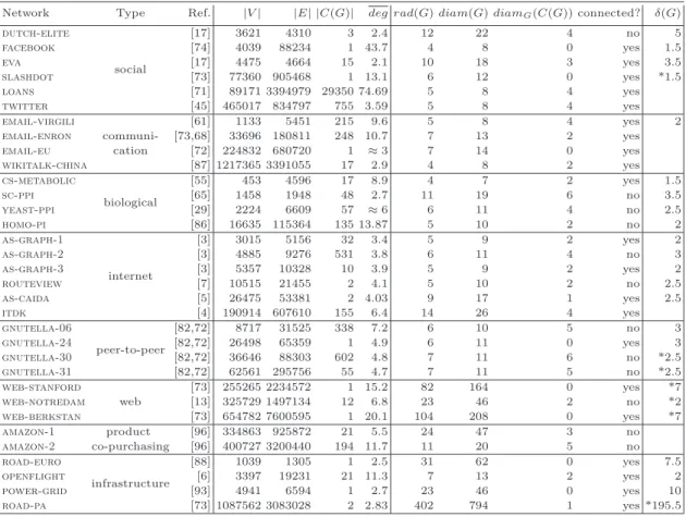
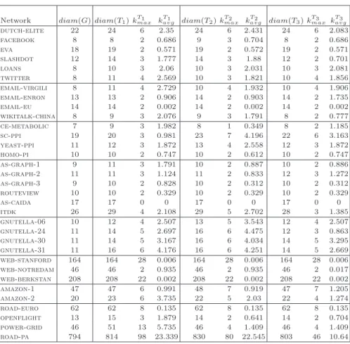
We apply our algorithms to six social networks, four email communication networks, four biological networks, six internet graphs, four peer-to-peer networks, three web networks, two product-co-purchasing networks, and four infrastructure networks. Most of the networks listed are part of the Stanford Large Network Dataset Collection (snap) and the Koblenz Network Collection (konect), and are available at [1] and [2]. Characteristics of these networks, such as the number of vertices and edges, the average degree, the radius and the diameter, are given in Table 1. The numbers listed in Table 1 are based on the largest connected component of each network, when the entire network is disconnected. We ignore the directions of the edges and remove all self-loops from each network. Additionally, in Table 1, for each network we report the size (as the number of vertices) of its center C(G). We also analyze the diameter and the connectivity of the center of each network. The diameter of the center diamG(C(G)) is defined as the maximum distance between any
two central vertices in the graph. In the last column of Table 1, we report the Gromov hyperbolicity δ of majority of networks2. Computing the hyperbolicity of a graph is computationally expensive; therefore, we
provide the exact δ values for the smaller networks (those with |V | ≤ 30K) in our dataset (in some cases, the algorithm proposed in [41] was used). For some larger networks, the approximated δ-hyperbolicity values listed in Table 1 are as reported in [67]3. Most networks that we included in our dataset are hyperbolic.
However, for comparison reasons, we included also a few infrastructure networks that are known to lack the hyperbolicity property.
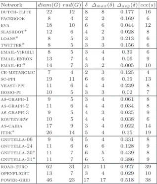
5.1 Estimation of Eccentricities
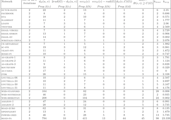
Following Proposition 2, for each graph in our dataset, we found a pair u, v of mutually distant vertices. In column two of Table 2, we report on how many BF S sweeps of a graph were needed to locate u and
v. Interestingly, for almost all graphs (28 out 33) only two sweeps were sufficient. For four other graphs
(including road-pa network whose hyperbolicity is large) three sweeps were needed, and only for one graph (power-grid network) we needed four sweeps.
2
All δ-hyperbolicity values listed in Table 1 were computed using Gromov’s four-point condition definition. As mentioned in [59,60], geodesic triangles of geodesic δ-hyperbolic spaces are 4δ-thin.
3
For web-stanford and web-berkstan, [67] gives 1.5 and 2, respectively, as estimates on the hyperbolicities. However, the sampling method they used seems to be not very accurate. According to [76], the hyperbolicities are at least 7 for both graphs.
Network Type Ref. |V | |E| |C(G)| deg rad(G) diam(G) diamG(C(G)) connected? δ(G) dutch-elite social [17] 3621 4310 3 2.4 12 22 4 no 5 facebook [74] 4039 88234 1 43.7 4 8 0 yes 1.5 eva [17] 4475 4664 15 2.1 10 18 3 yes 3.5 slashdot [73] 77360 905468 1 13.1 6 12 0 yes *1.5 loans [71] 89171 3394979 29350 74.69 5 8 4 yes twitter [45] 465017 834797 755 3.59 5 8 4 yes email-virgili [61] 1133 5451 215 9.6 5 8 4 yes 2 email-enron communi- [73,68] 33696 180811 248 10.7 7 13 2 yes email-eu cation [72] 224832 680720 1 ≈ 3 7 14 0 yes wikitalk-china [87] 1217365 3391055 17 2.9 4 8 2 yes cs-metabolic biological [55] 453 4596 17 8.9 4 7 2 yes 1.5 sc-ppi [65] 1458 1948 48 2.7 11 19 6 no 3.5 yeast-ppi [29] 2224 6609 57 ≈ 6 6 11 4 no 2.5 homo-pi [86] 16635 115364 135 13.87 5 10 2 no 2 as-graph-1 internet [3] 3015 5156 32 3.4 5 9 2 yes 2 as-graph-2 [3] 4885 9276 531 3.8 6 11 4 no 3 as-graph-3 [3] 5357 10328 10 3.9 5 9 2 yes 2 routeview [7] 10515 21455 2 4.1 5 10 2 no 2.5 as-caida [5] 26475 53381 2 4.03 9 17 1 yes 2.5 itdk [4] 190914 607610 155 6.4 14 26 4 yes gnutella-06 peer-to-peer [82,72] 8717 31525 338 7.2 6 10 5 no 3 gnutella-24 [82,72] 26498 65359 1 4.9 6 11 0 yes 3 gnutella-30 [82,72] 36646 88303 602 4.8 7 11 6 no *2.5 gnutella-31 [82,72] 62561 295756 55 4.7 7 11 5 no *2.5 web-stanford web [73] 255265 2234572 1 15.2 82 164 0 yes *7 web-notredam [13] 325729 1497134 12 6.8 23 46 2 no *2 web-berkstan [73] 654782 7600595 1 20.1 104 208 0 yes *7 amazon-1 product [96] 334863 925872 21 5.5 24 47 3 no amazon-2 co-purchasing [96] 400727 3200440 194 11.7 11 20 5 no road-euro infrastructure [88] 1039 1305 1 2.5 31 62 0 yes 7.5 openflight [6] 3397 19231 21 11.3 7 13 2 yes 2 power-grid [93] 4941 6594 1 2.7 23 46 0 yes 10 road-pa [73] 1087562 3083028 2 2.83 402 794 1 yes *195.5
Table 1. Statistics of the analyzed networks: |V | is the number of vertices, |E| is the number of edges;
|C(G)| is the number of central vertices; deg is the average degree; rad(G) is the graph’s radius; diam(G) is the graph’s diameter; diamG(C(G)) is the diameter of the graph’s center; ”connected?” indicates whether
or not the center of the graph is connected; δ(G) is the graph’s hyperbolicity. Hyperbolicity values marked with asterisks are approximate.
In column four of Table 2, we report for each graph G the difference between 2rad(G) and dG(u, v).
Proposition 2(c) says that the difference must be at most 2δ + 1, where δ is the thinness of geodesic triangles in G. Actually, for large number (27 out of 33) of graphs in our dataset, the difference is at most two. Five other graphs have the difference equal to 3, and only road-pa network has the difference equal to 10. We have dG(u, v) = diam(G) for 27 graphs in our dataset, including road-pa network whose geodesic triangles
thinness is at least 196. For remaining six graphs dG(u, v) = diam(G) − 1 holds.
We also analyzed the quality of a middle vertex c of a randomly picked shortest path between mutually distant vertices u and v. Proposition 2 states that eccG(c) is close to rad(G) and c is not too far from the
graph’s center C(G). Table 2 lists the properties of the selected middle vertex c. In almost all graphs, vertex c belongs to the center C(G) or is at distance one or two from C(G). Even in graphs with eccG(c)−rad(G) > 2
(power-grid and road-pa), the value eccG(c) − rad(G) is smaller than what is suggested by Proposition
2(b). It is also clear from Table 2 that c is not too far from any vertex in C(G) (look at the radius i of the ball B(c, i) required to include C(G)). In all graphs, i is much smaller than 2δ + 1 (indicated in Proposition 2(d)).
Following Theorem 1, for each graph G = (V, E) in our dataset, we constructed an arbitrary BF S(c)-tree
T1 = (V, E′), rooted at vertex c, and analyzed how well T1 preserves or approximates the eccentricities of
vertices in G. By Theorem 1, eccG(v) ≤ eccT1(v) ≤ eccG(v)+3δ+1 holds for every v ∈ V . In our experiments,
for each graph G and the constructed for it BF S(c)-tree T1, we computed kmax := maxv∈V{eccT1(v) −
eccG(v)} (maximum distortion) and kavg:= n1Pv∈V eccT1(v)−eccG(v) (average distortion). For most graphs
(see Table 2), the value of kmaxis small: kmax= 0 for one graph, kmax= 2 for eight graphs, kmax= 3 for nine
Network No. of BFS
iterations dG(u, v) 2rad(G) − dG(u, v) eccG(c) eccG(c) − rad(G) dG(c, C(G))
min i :
B(c, i) ⊇ C(G)kmax kavg Prop.2(c) Prop.2(c) Prop.2(b) Prop.2(b) Prop.2(d)
dutch-elite 2 22 2 13 1 1 3 6 2.35 facebook 2 8 0 4 0 0 0 2 0.686 eva 2 18 2 10 0 0 2 2 0.571 slashdot 2 11 1 7 1 2 2 3 1.777 loans 2 7 3 5 0 0 3 3 2.06 twitter 2 8 2 6 1 1 3 4 2.569 email-virgili 2 7 3 6 1 1 3 4 2.729 email-enron 2 13 1 7 0 0 2 2 0.906 email-eu 2 14 0 7 0 0 0 2 0.002 wikitalk-china 2 7 1 5 1 1 2 3 2.076 ce-metabolic 2 7 1 5 1 1 2 3 1.982 sc-ppi 3 19 3 12 1 2 6 3 0.981 yeast-ppi 3 11 1 6 0 0 3 3 1.872 homo-pi 2 10 0 5 0 0 2 2 0.747 as-graph-1 2 8 2 6 1 1 2 3 1.791 as-graph-2 3 11 1 6 0 0 3 3 1.124 as-graph-3 2 9 1 5 0 0 2 2 0.828 routeview 2 10 0 5 0 0 2 2 0.329 as-caida 2 17 1 9 0 0 1 0 0 itdk 2 26 2 15 1 1 3 4 2.108 gnutella-06 2 10 2 6 0 0 4 4 2.507 gnutella-24 2 10 2 7 1 1 1 5 2.697 gnutella-30 2 11 3 7 0 0 5 5 3.167 gnutella-31 2 11 3 8 1 2 5 6 4.176 web-stanford 2 164 0 82 0 0 0 28 0.006 web-notredam 2 46 0 23 0 0 2 2 0.935 web-berkstan 2 208 0 104 0 0 0 22 0.002 amazon-1 2 47 1 24 0 0 2 6 0.991 amazon-2 2 20 2 12 1 2 5 6 3.735 road-euro 2 62 0 31 0 0 0 8 0.135 openflight 2 13 1 8 1 1 2 3 1.879 power-grid 4 46 0 28 5 8 8 13 5.735 road-pa 3 794 10 415 13 44 45 98 23.339
Table 2. Qualities of a pair of mutually distant vertices u and v, of a middle vertex c of a (u, v)-geodesic,
and of a BF S(c)-tree T1 rooted at vertex c. ”No. of BFS iterations“ indicates how many
breadth-first-search iterations were needed to obtain a pair of mutually distant vertices u and v. For each vertex x ∈ V ,
k(x) := eccT1(x) − eccG(x). Also, kmax:= maxx∈V k(x) and kavg:=
1
n
P
x∈V k(x).
distortion kavg is much smaller than kmaxfor all graphs. In fact, kavg< 3 in all but five graphs
(gnutella-30, gnutella-31, amazon-2, power-grid, and road-pa). In graphs with high kmax, close inspection
reveals that only small percent of vertices achieve this maximum. For example, in graph web-stanford,
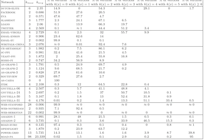
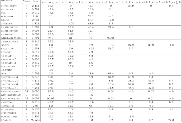
kmax= 28 was only achieved by 17 vertices. The distributions of the values of k(v) := eccT1(v) − eccG(v) of
all graphs are listed in Table 6 (see Appendix).
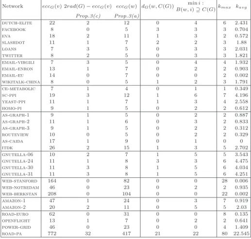
Similar experiments were performed following Proposition 3. For each graph G in our dataset, we picked a random vertex u ∈ V and a random vertex v ∈ F (u). Then, we identified in a randomly picked (u, v)-geodesic a vertex w at distance rad(G) from v. We did not consider a vertex c defined in Proposition 3(d) since, for majority of graphs in our dataset, c will be a middle vertex of a geodesic between two mutually distant vertices, and working with c we will duplicate previous experiments. Recall that for majority of our graphs (as found in our experiments) two BFS sweeps already identify a pair of mutually distant vertices. We know from Proposition 3 that eccG(v) ≥ diam(G) − 2δ ≥ 2rad(G) − 4δ − 1 and eccG(w) ≤ rad(G) + δ. Our
experimental results are better than these theoretical bounds. In Table 3, we list eccentricities of v and w for each graph. In almost all graphs, the eccentricity of v is equal to the diameter diam(G). Only four graphs have eccG(v) = diam(G) − 1 and one graph (road-pa) has eccG(v) > diam(G) − 1. Vertex w is central for
21 graphs, has eccentricity equal to rad(G) + 1 for 10 graphs, has eccentricity equal to rad(G) + 2 for one graph, and only for one remaining graph (road-pa network, which has large hyperbolicity) its eccentricity is equal to rad(G) + 15. It turns out also (see columns five and six of Table 2) that vertex w either belongs to the center C(G) or is very close to the center. The only exception is again road-pa network where 2rad(G) − eccG(w) = 32 and d(w, C(G)) = 21.
Network eccG(v) 2rad(G) − eccG(v) eccG(w) dG(w, C(G)) min i : B(w, i) ⊇ C(G)kmax kavg Prop.3(c) Prop.3(a) dutch-elite 22 2 12 0 4 6 2.431 facebook 8 0 5 3 3 3 0.704 eva 18 2 11 1 3 2 0.572 slashdot 11 1 7 2 2 3 1.88 loans 7 3 5 0 3 3 2.031 twitter 8 2 5 0 3 3 1.821 email-virgili 7 3 5 0 4 4 1.932 email-enron 13 1 7 0 2 2 0.903 email-eu 14 0 7 0 0 2 0.002 wikitalk-china 8 0 5 1 2 3 1.791 ce-metabolic 7 1 4 0 1 1 0.349 sc-ppi 19 3 12 1 6 7 4.196 yeast-ppi 11 1 7 1 3 4 2.558 homo-pi 9 1 5 0 2 2 0.612 as-graph-1 9 1 5 0 2 2 0.887 as-graph-2 11 1 6 0 3 2 0.833 as-graph-3 9 1 5 0 2 2 0.312 routeview 10 0 5 0 2 2 0.329 as-caida 17 1 9 0 1 0 0 itdk 26 2 15 1 3 5 2.702 gnutella-06 10 2 7 1 5 5 3.543 gnutella-24 11 1 8 3 3 6 4.475 gnutella-30 11 3 8 1 5 6 4.034 gnutella-31 11 3 8 1 5 6 4.251 web-stanford 164 0 82 0 0 28 0.006 web-notredam 46 0 23 0 2 2 0.935 web-berkstan 208 0 104 0 0 22 0.002 amazon-1 47 1 24 0 3 7 0.919 amazon-2 20 2 11 0 5 5 2.03 road-euro 62 0 31 0 0 8 0.135 openflight 13 1 7 0 2 2 0.641 power-grid 46 0 23 0 0 4 1.409 road-pa 772 32 417 21 22 80 22.545
Table 3. Qualities of a vertex v most distant from a random vertex u, of a vertex w of a (u, v)-geodesic
at distance rad(G) from v, and of a BF S(w)-tree T2 rooted at vertex w. For each vertex x ∈ V , k(x) := eccT2(x) − eccG(x). Also, kmax:= maxx∈Vk(x) and kavg:=
1
n
P
x∈Vk(x).
For every graph G = (V, E) in our dataset, we constructed also an arbitrary BF S(w)-tree T2= (V, E′),
rooted at vertex w, and analyzed how well T2 preserves or approximates the eccentricities of vertices in G.
The value of kmax is at most five for 23 graphs. The average distortion kavg is much smaller than kmax in
all graphs. The distributions of the values of k(x) for all graphs are presented in Table 7 (see Appendix). In Table 4, we compare these two eccentricity approximating spanning trees T1 and T2 with each other
and with a third BF S(c∗)-tree T3which we have constructed starting from a randomly chosen central vertex c∗∈ C(G).
For each graph in the dataset, three values of kmax (kmaxT1 , kmaxT2 and kTmax3 ) and three values of kavg
(kT1
avg, kTavg2 and kTavg3 ) are listed. We observe that the smallest kmax (out of three) is achieved by tree T3 in
28 graphs, by tree T2in 20 graphs and by tree T1in 20 graphs (in 14 graphs, the smallest kmaxis achieved
by all three trees). The difference between the largest and the smallest kmaxof a graph is at most one for 26
graphs in the dataset. The largest difference is observed for road-pa network: the largest kmax(98) is given
by tree T1, the smallest kmax(46) is given by tree T3. Two other graphs have the difference larger than three:
for sc-ppi network, the largest kmax (7) is given by tree T2, the smallest kmax (3) is given by tree T1; for
power-grid network, the largest kmax(13) is given by tree T1, the smallest kmax(4) is shared by remaining
trees T2, T3. Overall, we conclude that kmax values for trees T1 and T2 are comparable and generally can
be slightly worse than those for tree T3. Similar observations hold also for the average distortion kavg. Note,
however, that for construction of trees T2and T3 one needs to know rad(G) or a central vertex of G, which
Network diam(G) diam(T1) kmaxT1 kT1avg diam(T2) kmaxT2 kT2avg diam(T3) kmaxT3 kT3avg dutch-elite 22 24 6 2.35 24 6 2.431 24 6 2.083 facebook 8 8 2 0.686 9 3 0.704 8 2 0.686 eva 18 19 2 0.571 19 2 0.572 19 2 0.571 slashdot 12 14 3 1.777 14 3 1.88 12 2 0.701 loans 8 10 3 2.06 10 3 2.031 10 3 2.081 twitter 8 11 4 2.569 10 3 1.821 10 4 1.856 email-virgili 8 11 4 2.729 10 4 1.932 10 4 1.906 email-enron 13 13 2 0.906 14 2 0.903 14 2 1.735 email-eu 14 14 2 0.002 14 2 0.002 14 2 0.002 wikitalk-china 8 9 3 2.076 9 3 1.791 8 2 0.777 ce-metabolic 7 9 3 1.982 8 1 0.349 8 2 1.185 sc-ppi 19 20 3 0.981 23 7 4.196 22 6 3.163 yeast-ppi 11 12 3 1.872 13 4 2.558 12 3 1.872 homo-pi 10 10 2 0.747 10 2 0.612 10 2 0.747 as-graph-1 9 11 3 1.791 10 2 0.887 10 2 0.886 as-graph-2 11 11 3 1.124 11 2 0.833 12 3 1.272 as-graph-3 9 10 2 0.828 10 2 0.312 10 2 0.312 routeview 10 10 2 0.329 10 2 0.329 10 2 0.329 as-caida 17 17 0 0 17 0 0 17 0 0 itdk 26 29 4 2.108 29 5 2.702 28 3 1.385 gnutella-06 10 12 4 2.507 13 5 3.543 12 4 2.507 gnutella-24 11 14 5 2.697 16 6 4.475 12 3 0.863 gnutella-30 11 14 5 3.167 16 6 4.034 14 5 3.295 gnutella-31 11 16 6 4.176 16 6 4.251 14 5 2.669 web-stanford 164 164 28 0.006 164 28 0.006 164 28 0.006 web-notredam 46 46 2 0.935 46 2 0.935 46 2 0.017 web-berkstan 208 208 22 0.002 208 22 0.002 208 22 0.002 amazon-1 47 47 6 0.991 48 7 0.919 47 7 1.205 amazon-2 20 23 6 3.735 22 5 2.03 22 4 1.274 road-euro 62 62 8 0.135 62 8 0.135 62 8 0.135 openflight 13 15 3 1.879 14 2 0.641 14 2 0.704 power-grid 46 51 13 5.735 46 4 1.409 46 4 1.409 road-pa 794 814 98 23.339 830 80 22.545 803 46 10.64
Table 4. Comparison of three BFS-trees T1, T2 and T3. T3 is a BF S(c∗)-tree rooted at a randomly picked
central vertex c∗∈ C(G).
5.2 Estimation of Distances
Following Theorem 3, we experimented also on how well our approach approximates the distances in graphs from our dataset. To analyze the quality of approximation provided by our method for a given graph
G = (V, E), for every δ := 0, 1, 2, . . . , we computed an estimate bdδ(x, y) on dG(x, y) and the error ∆xy(δ) =
b
dδ(x, y) − dG(x, y) for all x, y ∈ V . In Table 5, we report ∆max(δ) = maxx,y∈V∆xy(δ) and ∆avg(δ) =
1
n2
P
x,y∈V ∆xy(δ) for the smallest δ such that ∆max(δ) ≤ δ + 1. We omitted some very large graphs in this
experiment. For some other large graphs, we did only sampling; we calculated ∆max(δ) and ∆avg(δ) based
only on a set of sampled vertices. We sampled vertices that are most distant from the root. The number of sampled vertices ranged from 10 to 100 in each network. For all networks investigated, the average error
∆avg(δ) was very small, less that 1 even for infrastructure networks. That is, the maximum error ∆max(δ)
was realized on a very small number of vertex pairs. The maximum error ∆max(δ) was 2 for three networks,
was 3 for five networks, was 4 for ten networks (including infrastructure network openflight), and was at most 6 for all except one social network dutch-elite and two infrastructure networks: road-euro and power-grid. The largest ∆max(δ) value had expectedly power-grid network whose hyperbolicity is 10. Acknowledgements
The research of V.C., M.H., and Y.V. was supported by ANR project DISTANCIA (ANR-17-CE40-0015).