A Simple and Efficient Method for Computing Data Cubes

HAL Id: hal-01796032

https://hal-amu.archives-ouvertes.fr/hal-01796032

Submitted on 18 May 2018

HAL is a multi-disciplinary open access

archive for the deposit and dissemination of

sci-entific research documents, whether they are

pub-lished or not. The documents may come from

teaching and research institutions in France or

abroad, or from public or private research centers.

L’archive ouverte pluridisciplinaire HAL, est

destinée au dépôt et à la diffusion de documents

scientifiques de niveau recherche, publiés ou non,

émanant des établissements d’enseignement et de

recherche français ou étrangers, des laboratoires

publics ou privés.

Viet Phanluong

To cite this version:

Viet Phanluong. A Simple and Efficient Method for Computing Data Cubes. INNOV 2015 : The

Fourth International Conference on Communications, Computation, Networks and Technologies, Nov

2015, Barcelona, Spain. �hal-01796032�

A Simple and Efficient Method for Computing Data Cubes

Abstract—Based on a construction of the power set of the

fact table schemes, this paper presents an approach to represent and to compute data cubes using a prefix tree structure for the storage of cuboids. Though the approach is simple, the experimental results show that it is efficient in run time and storage space.

Keywords-Data warehouse; Data cube; Data mining. I. INTRODUCTION

In data warehouse, a data cube of a fact table with n dimensions and m measures can be seen as the result of the set of the Structured Query Language (SQL) group-by queries over the power set of dimensions, with aggregate functions over the measures. The result of each group-by query is an aggregate view, called a cuboid, of the fact table. The concept of data cube represents important interests to business decision as it provides aggregate views of measures over multiple combinations of dimensions. As the number of cuboids in a data cube is exponential to the number of dimensions of the fact table, when the fact table is big, computing a cuboid is critical and computing all cuboids of a data cube is exponentially cost in time [1][5]. To improve the response time, the data cube is usually precomputed and stored on disks [6]. However, storing all the data cube is exponential in space. Research in Online Analytical Processing (OLAP) focuses important effort for efficient methods of computation and representation of data cubes.

A. Related work

There are approaches that represent data cubes approx-imately or partially [9][10][16][18]. The other approaches search to represent the entire data cube with efficient methods to compute and to store the cube [2][7][21]. The computing time and storage space can be minimized by re-ducing redundancies between tuples in cuboids [20] or based on equivalence relations defined on aggregate functions [11][15] or on the concept of closed itemsets in frequent itemset mining [14] or by coalescing the storage of tuples in cuboids [19].

In the approaches to efficiently compute and store the cube, the computation is usually organized over the complete lattice of subschemes of the fact table dimension scheme, in

such a way the run time and the storage space can be opti-mized by reducing redundancies [2][8][11][12][13][15][17]. The computation can traverse the complete lattice in a top-down or bottom-up manner. [7][16]. For grouping tuples to create cuboids, the sort operation can be used to reorganize tuples: tuples are grouped over the prefix of their scheme and the aggregate functions are applied over the measures. By grouping tuples, the fact table can be horizontally parti-tioned, each partition can be fixed in memory, and the cube computation can be modularized.

To optimize the cuboid construction, in top-down methods [7][20], the cuboids over the subschemes on a path from the top to the bottom in the complete lattice can be built in only one lecture of the fact table sorted over the largest scheme of the path. An aggregate filter is used for each subscheme. The filter contains, at each time, only one tuple over the subscheme with the current value of aggregated measures (or a non aggregated mark). When reading a new tuple of the fact table, if over the subscheme, the new tuple has the same value as the filter, then only the value of the aggregated measures is updated. Otherwise, the current content of the filter is flushed out to disk, and before the new tuple passes into the filter, the subtuple over the next subscheme (next on the path from the top to the bottom) goes into the next subscheme filter.

To minimize the storage space of a cuboid, only ag-gregated subtuples with agag-gregated measures are directly stored on disk. Non-aggregated subtuples are not stored but represented by references to the (sub)tuples where the non aggregated tuples are originated.

The bottom-up methods [11][13][15][20] walk the paths from the bottom to the top in the complete lattice, beginning with the empty node (corresponding to the cuboid with no dimension). For each path, let T0 be the scheme at the bottom node and Tnthe scheme at of the top node of the path (not necessary the bottom and the top of the lattice, as each node is visited only once). These methods begin by sorting the fact table over T0and by this, the fact table is partitioned into groups over T0. To minimize storage space, for each one of these groups, the following depth-first recursive process is applied [20].

If the group is single, then the only element of the group is represented by a reference to the corresponding tuple in

the fact table, and there is no further process: the recursive cuboid construction is pruned.

Otherwise, an aggregated tuple is created in the cuboid over T0 and the group is sorted over the next scheme T1 in the path (with larger scheme) to be partitioned into sub-groups. The creation of a real tuple or a reference in the cuboid corresponding to each subgroup over T1is similar to what we have done when building the cuboid over T0.

When the recursive process is pruned at a node Ti,0 ≤

i ≤ n, or reaches to Tn, it resumes with the next group of the partition over T0, until all groups of the partition are processed. The construction resumes with the next path, until all paths of the complete lattice are processed, and all cuboids are built.

Note that in the above optimized bottom-up method, in all cuboids, if references exist, they refer directly to tuples in the fact table, not to tuples in other cuboids. This method, named Totally-Redundant-Segment BottomUpCube (TRS-BUC), is reported in [20] as a method that dominates or nearly dominates its competitors in all aspects of the data cube problem: fast computation of a fully materialized cube in compressed form, incrementally updateable, and quick query response time.

B. Contribution

This paper presents a simple and efficient approach to compute and to represent data cube without sorting the fact table or any part of it, neither partitioning the fact table, nor computing the complete lattice of subschemes, nor sophisticated techniques to implement direct or indirect references of tuples in cuboids. The efficient representation of data cube is not only a compact representation of all cuboids of the data cube, but also an efficient method to get the original cuboids from the compact representation. The main ideas of the proposed approach are:

1) Among the cuboids of a data cube, there are ones that can be easily and rapidly get from the others, with no important computing time. We call the latters the prime and next-prime cuboids. These cuboids will be computed and stored on disks.

2) The prime and next-prime cuboids are computed and stored on disk using a prefix tree structure for compact representation. To improve the efficiency of research through the prefix tree, this work integrates the binary search tree into the prefix tree.

3) To compute the prime and next-prime cuboids, this work proposes a running scheme in which the computation of the current cuboids can be speeded up by using the previously computed cuboids.

The paper is organized as follows. Section 2 introduces the concept of the prime and next-prime schemes and cuboids. Section 3 presents the structure of the integrated binary search prefix tree used to store cuboids. Section 4 presents the running scheme to compute the prime and next-prime

cuboids and shows how to efficiently get any other cuboids from the prime and next-prime cuboids. Section 5 reports the experimentation results. Finally, conclusion and further work are in Section 6.

II. PRIME AND NEXT-PRIME CUBOIDS

This section defines the main concepts of the present approach to compute and to represent data cubes.

A. A structure of the power set

A data cube over a scheme S is the set of cuboids built over all subsets of S, that is the power set of S. As in most of existing work, attributes are encoded in integer, let us consider S = {1, 2, ..., n}, n ≥ 1. The power set of S can be recursively defined as follows.

1) The power set of S0= ∅ (the empty set) is P0= {∅}. 2) For n≥ 1, the power set of Sn= {1, 2, ..., n} can be defined recursively as follows:

Pn= Pn₋1∪ {X ∪ {n} | X ∈ Pn₋1} (1)

Pn is the union of Pn

−1(the power set of Sn−1) and the set of which each element is built by adding n to each element of Pn₋1. Let us call Pn₋1the first-half power set of Snand the second operand the last-half power set of Sn.

Example: For n= 3, S3= {1, 2, 3}, we have:

P0= {∅}, P1= {∅, {1}}, P2= {∅, {1}, {2}, {1, 2}},

P3= {∅, {1}, {2}, {1, 2}, {3}, {1, 3}, {2, 3}, {1, 2, 3}}. The last-half power set of S3 is:

{{3}, {1, 3}, {2, 3}, {1, 2, 3}}.

B. Last-half data cube and first-half data cube

Consider a fact table R (a relational data table) over a dimension scheme Sn = {1, 2, ..., n}. In view of the first-half and the last-half power set, suppose that X = x1, ..., xi ⊆ Sn is an element of the first-half power set of Sn. Let Y be the smallest element of the last-half power set of Sn that contains X. Then, Y = X ∪ {n}. If the cuboid over Y is already computed in the attribute order x1, ..., xi, n, then the cuboid over X = x1, ..., xi can be done by a simple sequential reading of the cuboid over Y to get data for the cuboid over X. So, we call:

– A scheme in the last-half power set a prime scheme and a cuboid over a prime scheme a prime cuboid. Note that all prime schemes contain the last attribute n and any scheme that contains attribute n is a prime scheme.

– For efficient computing, the prime cuboids are computed by pairs with one dataset access for each pair. Such a pair is composed of two prime cuboids. The scheme of the first one has attribute1 and the scheme of the second one is obtained from the scheme of the first one by deleting attribute1. We call the second prime cuboid the next-prime cuboid.

– The set of all cuboids over the prime (or next-prime) schemes is called the last-half data cube. The set of all remaining cuboids is called the first-half data cube. In this

TABLE I. FACT TABLE R1 RowId A B C D M 1 a2 b1 c2 d2 m1 2 a3 b2 c2 d2 m2 3 a1 b1 c1 d1 m1 4 a1 b1 c2 d1 m3 5 a3 b3 c2 d3 m2

approach, the last-half data cube is computed and stored on disks. Cuboids in the first-half data cube are computed as queries based on the last-half data cube.

III. INTEGRATED BINARY SEARCH PREFIX TREE The prefix tree structure offers a compact storage for tuples: the common prefix of tuples is stored once. So, there is no redundancy in storage. Despite the compact structure of the prefix tree, if the same prefix has a large set of different suffixes, then the search time in the set of suffixes can be important. To tackle it, this work proposes to integrate the binary search tree into the prefix structure. The integrated structure, called the binary search prefix tree (BSPT), is used to store tuples of cuboids. With this structure, tuples with the same prefix are stored as follows:

– The prefix is stored once.

– The suffixes of those tuples are organized in siblings and stored in a binary search tree.

Precisely, in C language, the structure is defined by : typedef struct bsptree Bsptree; // Binary search prefix tree struct bsptree{ Elt data; // data at a node

Ltid *ltid; // list of RowIds Bsptree *son, *lsib, *rsib; };

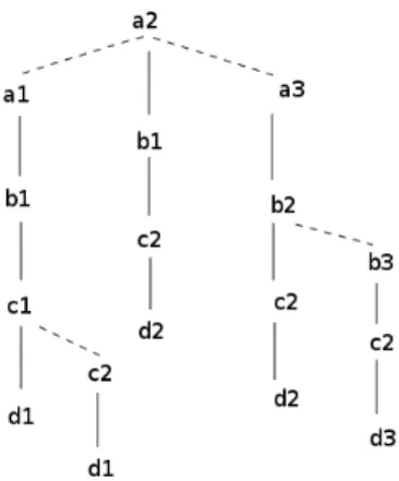
where son, lsib, and rsib represent respectively the son, the left and the right siblings of nodes. The field ltid is reserved for the list of tuple identifiers (RowId) associated with nodes. For efficient memory use, ltid is stored only at the last node of each path in the BSPT. With this representation, each binary search tree contains all siblings of a node in the normal prefix tree. For example, we have: – Table I represents the fact table R1 over the dimension scheme ABCD and a measure M .

– Figure 1 represents the BSPT of the tuples over the scheme ABCD of the fact table R1, where we suppose that with the same letter x, if i < j then xi < xj, e.g., a1 < a2 < a3. In Figure1, the continue lines represent the son links and the dash lines represent the lsib or rsib links.

The BSPT is saved to disk with the following format: level > suf f ix: ltids

where

– level is the length of the prefix part that the path has in common with its left neighbor,

– suffix is a list of elements, and

– ltids is a list of tuple identifiers (RowId).

Cuboids are built using the BSPT structure. The list of RowIds associated with the last node of each path allows

Figure 1. A binary search prefix tree

the aggregate of measures. For example, with the fact table in Table I, the cuboid over ABCD is saved on disk as the following. 0 > a1 b1 c1 d1 : 3 2 > c2 d1 : 4 0 > a2 b1 c2 d2 : 1 0 > a3 b2 c2 d2 : 2 1 > b3 c2 d3 : 5 A. Insertion of tuples in a BSPT

Algorithm Tuple2Ptree: Insert a tuple into a BSPT. Input: A BSPT represented by node P , a tuple ldata and

its list of tids lti.

Output: The tree P updated with ldata and lti. Method:

If (P is null) then

create P with P->data = head(ldata), P->son = P->lsib = P->rsib = NULL; if queue(ldata) is null then P->ltid =lti

else P->son = Tuple2Pree(P->son, queue(ldata), lti); Else if (P->data > head(ldata)) then

P->lsib=Tuple2Ptree(P->lsib, ldata,lti); else if (P->data < head(ldata)) then

P->rsib=Tuple2Ptree(P->rsib, ldata,lti); else if queue(ldata) is null then

P->ltid = insert(P->ltid, lti);

else P->son = Tuple2Ptree(P->son, queue(ldata), lti); return P;

In algorithm Tuple2Ptree, head(ldata) returns the first element of ldata and queue(ldata) returns the queue of ldata after removing head(ldata).

B. Grouping tuples using binary prefix tree

Algorithm Table2Ptree: Build a BSPT for a relational table. Input: A table R in which each tuple has a list of tids lti. Output: The BSPT P for R

Create an empty BSPT P;

For each tuple ldata in R with its list of tids lti do P = Tuple2Ptree(P, ldata, lti) done; Return P;

IV. COMPUTING THE LAST-HALF DATA CUBE Let S = {1, 2, ..., n} be the set of all dimensions of the fact table. To compute the last-half data cube:

– We begin by computing the first prime and next-prime cuboids based on the fact table, one over S and the other over S− {1}.

– Apart the first prime and next-prime cuboids (over S and S− {1}, respectively), for the current prime scheme X of size k (the number of all dimensions in X), the computation of the prime and next-prime cuboids over X and X−{1}, respectively, is based on a previously computed prime cuboid with the smallest scheme that contains X.

– To keep track of the computation, we keep the schemes of all computed prime cuboids in a list called the running scheme and denoted by RS. So, X is appended to RS (S is the first element added to RS). To build the RS, for the currently pointed scheme X in RS, for each dimension j∈ X, j 6= 1 and j 6= n (n is the last dimension of the fact table), we append X − {j} to RS, if X − {j} is not yet there.

More precisely, for computing the last-half data cube, we use algorithm LastHalf Cube.

Algorithm LastHalfCube

Input: A fact table R over scheme S of n dimensions. Output: The last-half data cube of R and the running

scheme RS.

Method:

0) RS = emptyset; // RS: Running Scheme 1) Append S to the RS;

2) Using Table2Tree and R to generate two cuboids over S and S - {1}, respectively;

3) Set cS to the first scheme in RS; // cS: current scheme 4) While cS has more than 2 attributes do

5) For each dimension d in cS, d6= 1 and d 6= n, do 6) Build a subscheme scS by deleting d from cS; 7) If scS is not yet in RS then append scS to RS, let

cubo be the cuboid over cS (already computed); If cubo is not yet in memory then load it in memory; 8) Using Tuple2Ptree and cubo to generate two cuboids

over scS and scS -{1}, respectively; 9) done;

10) Set cS to the next scheme in RS; 11) done;

12) Return RS;

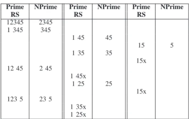
A. Example of running scheme

Table II shows the simplified execution of LastHalfCube on a table R over S= {1, 2, 3, 4, 5}: only the prime and the

TABLE II. GENERATION OF THE RUNNING SCHEME OVER S ={1, 2, 3, 4, 5}.

Prime NPrime Prime NPrime Prime NPrime

RS RS RS 12345 2345 1 345 345 1 45 45 15 5 1 35 35 15x 12 45 2 45 1 45x 1 25 25 15x 123 5 23 5 1 35x 1 25x

next-prime (NPrime) schemes of the cuboids computed by the algorithm are reported. The prime schemes appended to RS (Running Scheme) during the execution of LastHalfCube are in the columns named Prime/RS of Table II. The first prime schemes are in the first column Prime/RS, the next ones are in the second column Prime/RS, and the final ones are in the third column Prime/RS. The final state of RS is {12345, 1345, 1245, 1235, 145, 135, 125, 15}. In Table II the schemes marked with x (e.g., 145x) are those already added to RS and are not re-appended to RS.

For a fact table R over a scheme S of n dimensions, S = {1, 2, ..., n}, algorithm LastHalfCube generates RS with 2n₋2

subschemes. Indeed, we can see that all sub-schemes appended to RS have 1 as the first attribute and n as the last attribute. So, we can forget 1 and n from all those subschemes. By this, we can consider that the first subscheme added to RS is2, ..., n − 1. Over 2, ..., n − 1, we have only one subscheme of size n− 2 (Cn₋2

n₋2). In the loop For at point 5 of LastHalfCube, alternatively each attribute from 2 to n− 1 is deleted to generate a subscheme of size n− 3. By doing this, we can consider as, in each iteration, we build a subscheme over n−3 different attributes selected among n− 2 attributes. So, we build Cn

−3

n₋2 subschemes. So on, until the subscheme{1, n} (corresponding to the empty scheme after forgetting1 and n) is added to RS. As

Cn−2 n₋2+ C n −3 n₋2+ .... + C 0 n −2= 2 n −2

By adding the corresponding next-prime schemes, LastHalfCube generates 2n

−1 _{different subschemes. Thus,} algorithm LastHalfCube computes 2n

−1 _{prime and} next-prime cuboids.

B. Data Cube representation

For a fact table R over a dimension scheme S = {1, 2, ..., n} with measures M1, ..., Mk, the data cube of R is represented by the three following elements:

1) The running scheme (RS): The list of the prime schemes over S. Each prime scheme has an identifier

number that allows to locate the files corresponding to the prime and next-prime cuboids in the last-half data cube.

2) The last-half data cube of which the cuboids are precomputed and stored on disks using the format to store the BSPT.

3) A relational table over RowId, M1, ..., Mk that repre-sents the measures associated with each tuple of R.

Clearly, such a representation reduces about 50% space of the entire data cube, as it represents the last-half data cube in the BSPT format.

C. Computing the first-half data cube

Let X be a scheme in the first-half power set of S = {1, 2, ..., n}. For computing the cuboid over X, we base on the precomputed last-half data cube over S. The computation is processed as follows, where lti(t) denotes the list of tids of a tuple t and p(t) the prefix of t over X.

Let C be the stored cuboid over X∪ {n}; Let t1 be the 1st tuple of C and ltids = lti(t1) ; For each next tuple t2 of C do

If the p(t2) = p(t1) then append lti(t2) to ltids, Else{

Write p(t1) : ltids to the cuboid over X; t1 = t2; ltids = lti(t1);

} Done;

V. EXPERIMENTAL RESULTS

The present approach to represent and to compute data cubes is implemented in C and experimented on a laptop with 8 GB memory, Intel Core i5-3320 CPU @ 2.60 GHz x 4, 188 Go Disk, running Ubuntu 12.04 LTS. To get some ideas about the efficiency of the present ap-proach, we recall here the experimental results reported in [20] as references, because the work [20] has ex-perimented many existing and well known methods for computing and representing data cube as Partitioned-Cube (PC), Redundant-Segment-PC (PRS-PC), Partially-Redundant-Tuple-PC (PRT-PC), BottomUpCube (BUC), Bottom-Up-Base-Single-Tuple (BU-BST), and Totally-Redundant-Segment BottomUpCube (TRS-BUC). The ex-periments in [20] were run on a Pentium 4 (2.8 GHz) PC with 512 MB memory under Windows XP. The results were reported on real and synthetic datasets. In the present work, we limit our attention to only the real datasets: CovType [3] and SEP85L5 [4]. However, by reporting the results of [20], we do not want to really compare the present approach to TRS-BUC or others, as we do not have sufficient conditions to implement and to run these methods on the same system and machine.

CovType is a dataset of forest cover-types. It has ten dimensions and 581,012 tuples. The dimensions and their cardinality are: Horizontal-Distance-To-Fire-Points (5,827), Horizontal-Distance-To-Roadways (5,785),

TABLE III. EXPERIMENTAL RESULTS REPORTED IN [20]

CovType

Algorithms Storage space Construction time avg QRT

PC #12.5 Gb 1900 sec

PRT-PC #7.2 Gb 1400 sec

PRS-PC #2.2 Gb 1200 sec 3.5 sec

BUC #12.5 Gb 2900 sec 2 sec

BU-BST #2.3 Gb 350 sec

BU-BST+ #1.2 Gb 400 sec 1.3 sec

TRS-BUC #0.4 Gb 300 sec 0.7 sec

SEP85L

Algorithms Storage space Construction time avg QRT

PC #5.1 Gb 1300 sec

PRT-PC #3.3 Gb 1150 sec

PRS-PC #1.4 Gb 1100 sec 1.9 sec

BUC #5.1 Gb 1600 sec 1.1 sec

BU-BST #3.6 Gb 1200 sec

BU-BST+ #2.1 Gb 1300 sec 0.98 sec

TRS-BUC #1.2 Gb 1150 sec 0.5 sec

Elevation (1,978), Vertical-Distance-To-Hydrology (700), Horizontal-Distance-To-Hydrology (551), Aspect (361), Hillshade-3pm (255), Hillshade-9am (207), Hillshade-Noon (185), and Slope (67).

SEP85L is a weather dataset. It has nine dimensions and 1,015,367 tuples. The dimensions and their cardinality are: Station-Id (7,037), Longitude (352), Solar-Altitude (179), Latitude (152), Present-Weather (101), Day (30), Weather-Change-Code (10), Hour (8), and Brightness (2).

For greater efficiency, in the experiments of [20], the dimensions of the datasets are arranged in the decreas-ing order of the attribute domain cardinality. The same arrangement is done in the our experiments. Moreover, as most algorithms studied in [20] compute condensed cuboids, computing query in data cube needs additional cost. So, the results are reported in two parts: computing the condensed data cube and querying data cube. The former is reported with the construction time and storage space and the latter the average query response time.

Table III presents the experimental results approximately got from the graphs in [20], where “avg QRT” denotes the average query response time and “Construction time” denotes the time to construct the (condensed) data cube. However, [20] did not specify whether the construction time includes the time to read/write data to files.

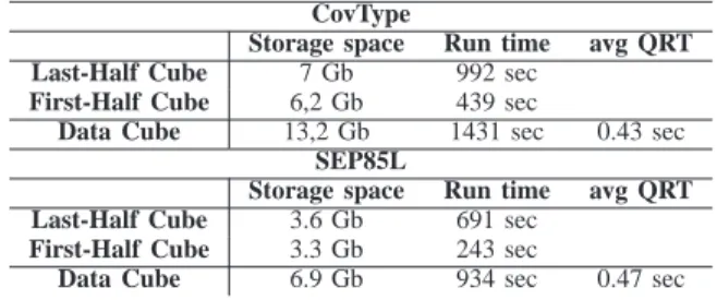
Table IV reports the results of the present work, where the term “run time” means the time from the start of the program to the time the last-half (or respectively, the first-half) data cube is completely constructed, including the time to read/write input/output files.

As we do not compute the condensed cuboids, but only compute the last-half data cube and use it to represent the data cube, we can consider that the last-half data cube corre-sponds somehow to the (condensed) representations of data cube in the other approaches, and computing the first-half data cube corresponds to querying data cube. In this view,

TABLE IV. EXPERIMENTAL RESULTS OF THIS WORK

CovType

Storage space Run time avg QRT Last-Half Cube 7 Gb 992 sec

First-Half Cube 6,2 Gb 439 sec

Data Cube 13,2 Gb 1431 sec 0.43 sec

SEP85L

Storage space Run time avg QRT Last-Half Cube 3.6 Gb 691 sec

First-Half Cube 3.3 Gb 243 sec

Data Cube 6.9 Gb 934 sec 0.47 sec

the average query response time corresponds to the average run time for computing a cuboid based on the precomputed and stored cuboids. That is, the average query response time for SEP85L is 243s/512 = 0.47 second and for CovType 439s/1024 = 0.43 second, because the cuboids in the last-half data cube are precomputed and stored, only querying on the first-half data cube needs computing. Though the compactness of the data cube representation by the present approach is not comparable to the compactness offered by TRS-BUC, it is in the range of other existing methods. It is similar for the run time to build the last-half data cube of CovType. However, the run time to build the entire (not only the last-half) data cube of SEP85L seems to be better than all other existing methods. On the average query response time, it seems that the present approach offers a competitive solution, because querying data cube is a repetitive operation and improving the average query response time is one of the important goals of research on data cube.

VI. CONCLUSION,REMARKS AND FURTHER WORK Essentially, this work represents a data cube by the last-half data cube: the set of cuboids over schemes that contain the last dimension of the fact table, called prime (or next-prime) cuboids. All other cuboids, those over schemes that do not contain the last dimension, are obtained by a simple projection of the corresponding cuboids in the last-half data cube. The binary search prefix tree (BSPT) structure is used to store cuboids in memory and on disk. Such a structure offers not only a compact representation of cuboids but also an efficient search of tuples. Building a cuboid in the last-half data cube is reduced to building a BSPT. Building a cuboid in the first-half data cube is reduced to copying the prefixes of the BSPT of the corresponding cuboid in the last-half data cube. The BSPT allows efficient group-by operation without previous sort operation on tuples in the fact table or in cuboids. With this advantage, we can think of the possibility of incremental construction of the last-half data cube and the possibility of updating the data cube when inserting new tuples in the fact table.

REFERENCES

[1] S. Agarwal et al., “On the computation of multidimensional aggregates”, Proc. of VLDB’96, pp. 506-521.

[2] V. Harinarayan, A. Rajaraman, and J. Ullman, “Implementing data cubes efficiently”, Proc. of SIGMOD’96, pp. 205-216. [3] J. A. Blackard, “The forest covertype dataset”, ftp://ftp. ics.uci.

edu/pub/machine-learning-databases/covtype, [retrieved: April, 2015].

[4] C. Hahn, S. Warren, and J. London, “Edited synoptic cloud re-ports from ships and land stations over the globe”, http://cdiac. esd.ornl.gov/cdiac/ndps/ndp026b.html, [retrieved: April, 2015]. [5] S. Chaudhuri and U. Dayal, “An Overview of Data Warehous-ing and OLAP Technology”, SIGMOD record 1997, 26 (1), pp. 65-74.

[6] J. Gray et al., “Data Cube: A Relational Aggregation Opera-tor Generalizing Group-by, Cross-Tab, and Sub-Totals”, Data Mining and Knowledge Discovery 1997 , 1 (1), pp. 29-53. [7] K. A. Ross and D. Srivastava, “Fast computation of sparse data

cubes”, Proc. of VLDB’97, pp. 116-125.

[8] Y. Zhao, P. Deshpande, and J. F. Naughton, “An array-based al-gorithm for simultaneous multidimensional aggregates”, Proc. of ACM SIGMOD’97, pp. 159-170.

[9] J. S. Vitter, M. Wang, and B. R. Iyer, “Data cube approxi-mation and histograms via wavelets”, Proc. of Int. Conf. on Information and Knowledge Management (CIKM’98), pp. 96-104.

[10] J. Han, J. Pei, G. Dong, and K. Wang, “Efficient Computation of Iceberg Cubes with Complex Measures”, Proc. of ACM SIGMOD’01, pp. 441-448.

[11] L. Lakshmanan, J. Pei, and J. Han, “Quotient cube: How to summarize the semantics of a data cube,” Proc. of VLDB’02, pp. 778-789.

[12] Y. Sismanis, A. Deligiannakis, N. Roussopoulos, and Y. Kotidis, “Dwarf: shrinking the petacube”, Proc. of ACM SIG-MOD’02, pp. 464-475.

[13] W. Wang, H. Lu, J. Feng, and J. X. Yu, “Condensed cube: an efficient approach to reducing data cube size”, Proc. of Int. Conf. on Data Engineering 2002, pp. 155-165.

[14] A. Casali, R. Cicchetti, and L. Lakhal, “Extracting semantics from data cubes using cube transversals and closures”, Proc. of Int. Conf. on Knowledge Discovery and Data Mining (KDD’03), pp. 69-78.

[15] L. Lakshmanan, J. Pei, and Y. Zhao, “QC-Trees: An Efficient Summary Structure for Semantic OLAP”, Proc. of ACM SIGMOD’03, pp. 64-75.

[16] D. Xin, J. Han, X. Li, and B. W. Wah, “Star-cubing: com-puting iceberg cubes by top-down and bottom-up integration”, Proc. of VLDB’03, pp. 476-487.

[17] Y. Feng, D. Agrawal, A. E. Abbadi, and A. Metwally, “Range cube: efficient cube computation by exploiting data correlation”, Proc. of Int. Conf. on Data Engineering 2004, pp. 658-670.

[18] Z. Shao, J. Han, and D. Xin, “Mm-cubing: computing iceberg cubes by factorizing the lattice space”, Proc. of Int. Conf. on Scientific and Statistical Database Management (SSDBM 2004), pp. 213-222.

[19] Y. Sismanis and N. Roussopoulos, “The complexity of fully materialized coalesced cubes”, Proc. of VLDB’04, pp. 540-551.

[20] K. Morfonios and Y. Ioannidis, “Supporting the Data Cube Lifecycle: The Power of ROLAP”, The VLDB Journal, 2008, 17(4), pp. 729-764.

[21] A. Casali, S. Nedjar, R. Cicchetti, L. Lakhal, and N. Novelli, “Lossless Reduction of Datacubes using Partitions”, In Int. Journal of Data Warehousing and Mining (IJDWM), 2009, Vol 5, Issue 1, pp. 18-35.