HAL Id: ensl-00358777
https://hal-ens-lyon.archives-ouvertes.fr/ensl-00358777
Submitted on 4 Feb 2009
HAL is a multi-disciplinary open access
archive for the deposit and dissemination of
sci-entific research documents, whether they are
pub-lished or not. The documents may come from
teaching and research institutions in France or
abroad, or from public or private research centers.
L’archive ouverte pluridisciplinaire HAL, est
destinée au dépôt et à la diffusion de documents
scientifiques de niveau recherche, publiés ou non,
émanant des établissements d’enseignement et de
recherche français ou étrangers, des laboratoires
publics ou privés.
Sparse time-frequency distributions of chirps from a
compressed sensing perspective
Patrick Flandrin, Pierre Borgnat
To cite this version:
Patrick Flandrin, Pierre Borgnat. Sparse time-frequency distributions of chirps from a compressed
sensing perspective. 8th IMA International Conference on Mathematics in Signal Processing, IMA,
Dec 2008, Cirencester, United Kingdom. �ensl-00358777�
Sparse time-frequency distributions of chirps
from a compressed sensing perspective
Patrick Flandrin & Pierre Borgnat
Universit´e de Lyon, ´Ecole Normale Sup´erieure de Lyon Laboratoire de Physique (UMR 5672 CNRS), 46, All´ee d’Italie, 69364 Lyon Cedex 07, France
Abstract
Considering that multicomponent chirp signals are sparse in the time-frequency domain, it is possible to attach to them highly localized distributions thanks to a compressed sensing approach based on very few measurements in the ambiguity plane. The principle of the technique is described, with emphasis on the choice of the measurement subset for which an optimality criterion is proposed.
1
Introduction
In the case of a multicomponent chirp signal of the form x(t) =
K
X
k=1
ak(t) eiϕk(t), (1)
an idealized representation amounts to distributing its energy along trajectories of the time-frequency (TF) plane according to ρ(t, f ) = K X k=1 a2 k(t) δ (f − ˙ϕk(t)/2π) . (2)
If the number of components of x(t) happens to be small, i.e., if — in a discrete-time setting — K ≪ M , where M is the number of frequency bins, this corresponds to a representation that is intrinsically sparse since, for a signal of length N , the TF matrix of total cardinality |ρ| = N M has at most KN ≪ |ρ| non-zero entries.
Some recent work [1] took advantage of this observation and proposed a new way of getting a sparse and sharply localized TF distribution of chirps on the basis of “compressed sensing” ideas [2]. The purpose of the present contribution is to go beyond the preliminary results reported in [1] and, in particular, to better address key questions related to a meaningful selection of the measurement subset on which the approach relies.
2
Rationale
It is well-known [3] that classical (quadratic) TF analysis offers a possibility of perfect localization on specific types of monocomponent chirps, while facing a trade-off between such a localization and the creation of spurious cross-terms in the case of multicomponent signals. Thorough analyses of this problem have been conducted (see, e.g., [4, 5, 6]), whose main result is that the signature of auto-terms of any TF distribution is mainly concentrated in the vicinity of the origin of the ambiguity plane, suggesting to build localized distributions on such contributions only so as to reduce the importance of cross-terms. From a standard perspective (i.e., Fourier inversion with no constraint), this however leads to a severe trade-off, the localization in the TF domain becoming all the more poor as the selected domain is shrunk in the ambiguity plane.
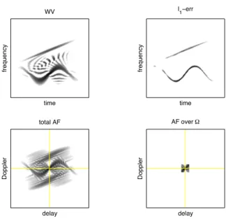
Assuming for the target TF distribution a model such as in eq. (2), a way out is however possible. Indeed, as illustrated in Fig. 1, the rationale is to exploit sparsity in the TF plane by making very few (incoherent) measurements in the ambiguity domain so as to get rid of most cross-terms, while
time fre q u e n cy ,-time fre q u e n cy l1!err delay 2 o p p le r total A7 delay 2 o p p le r A7 over !
Figure 1: Example with a 128 points 2-component signal — Top left: Wigner-Ville Distribution (WVD) of size 128 × 128. Bottom left: total ambiguity function (AF) of size 128 × 128, defined as the 2D Fourier transform of the WVD. Bottom right: restriction of the AF to a domain Ω consisting of 13 × 13
samples neighbouring the origin of the plane. Top right: minimum ℓ1-norm TF solution whose 2D Fourier
transform coincides with the AF over Ω, up to a ℓ2-norm approximation with ǫ = 0.05 kxk2.
constraining the inversion so as to guarantee that only few coefficients are significantly non-zero. From such a “compressed sensing” perspective (see, e.g., [2]), a better TF localization is thus expected to be obtained via the solving of the linear program
{min
ρ kρk1; kF{ρ} − Axk2≤ ǫ|(ξ,τ )∈Ω}, (3)
where ρ stands for the target distribution, F for the 2D Fourier transform operator, Axfor the ambiguity
function — classically computed as the 2D Fourier transform of the Wigner-Ville Distribution (WVD) [3] —, ǫ for a slack variable and Ω for some domain neighbouring the origin of the ambiguity plane. As discussed in [1], introducing in eq. (3) an approximate satisfaction of the constraint (in a combined ℓ1−ℓ2
sense) guarantees a smoother solution as compared to the oversparse, discontinuous solution that would be obtained with a strict equality (ǫ = 0).
3
Choosing the measurement subset
Fig. 1 evidences a dramatic improvement when switching from the WVD to the ℓ1-norm solution of
the program (3), in both terms of localization and cross-terms reduction1. However, such a result relies
heavily on the choice of the measurement subset Ω, raising the issue of how to choose it in an appropriate way.
3.1
Oracle
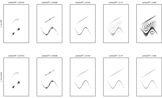
A qualitative appreciation can first be gained from a comparison with an “oracle” based on the assumed knowledge of the ideal distribution. In this case, the linear program (3) is run exactly as in Fig. 1, while replacing mutatis mutandis the WVD by the TF model (2). This is illustrated in Fig. 2, where an optimum cardinality |Ω|∗ is shown to exist, at least qualitatively, for trading off auto-terms localization
and cross-terms reduction.
At this point, it might be worth recalling that the approach described here differs from a reconstruction problem in the sense that there would be no point in exactly recovering the whole WVD from a limited set
1All the computations have been made in Matlab, with the Time-Frequency ToolBox (http://tftb.nongnu.org) for
l1 ! e rr ! W V card(!)/N2 = 0.00153 l1 ! e rr ! o ra cl e card(!)/N2 = 0.00153 card(!)/N2 = 0.00299 card(!)/N2 = 0.00299 card(!)/N2 = 0.0103 card(!)/N2 = 0.0103 card(!)/N2 = 0.147 card(!)/N2 = 0.147 card(!)/N2 = 0.984 card(!)/N2 = 0.984
Figure 2: Qualitative selection of the optimal cardinality |Ω| — Top row: TF solutions obtained from the WVD as in Fig. 1, for increasing values of |Ω|. The evolution shows that a too small cardinality does not permit to gain enough information about auto-terms whereas a too large one leads to take into account more and more undesired cross-terms, converging eventually to the actual WVD when the support of Ω identifies to the whole AF plane. Bottom row: companion “oracle” solutions obtained the same way, but based on the ideal distribution in place of the WVD. Comparison of both evolutions evidences that an
optimum cardinality |Ω|∗exists for trading off auto-terms localization and cross-terms reduction (about
1% of the AF support in the present case).
of measurements (in fact, such a perfect reconstruction is of course obtained when the entire ambiguity plane is chosen as the measurement domain, see Fig. 2). The situation is much more that of a construction problem in which is created some idealized object which does not exist per se prior optimization.
3.2
Optimum cardinality
Fig. 2 suggests that some “optimum” cardinality exists for trading-off localization and cross-terms, thus
calling for some automatic selection. Interpreting the way the ℓ1-solutions (WVD and oracle) evolve as
a function of |Ω|, one can say that essentially two regimes are observed. For small cardinalities, both behaviors happen to be quite similar, focusing primarily on the auto-terms of interest: in this respect, a measure of concentration such as the Shannon entropy can be a good indicator of performance. In a second stage, enlarging |Ω| is of little interest for auto-terms while letting cross-terms appear: in this regime, the entropy criterion can then be misleading since it may decrease not because of better localized auto-terms but rather of “spiky” structures due to the oscillatory nature of cross-terms.
In order to circumvent this drawback, it is therefore proposed to combine entropy (aimed at quantifying localization) with Total Variation (aimed at penalizing spiky structures) according to:
C = − Z Z +∞ −∞ |ρ|n(t, f ) log2|ρ|n(t, f ) dt df + λ Z Z +∞ −∞ s ∂ρn ∂t (t, f ) 2 + ∂ρn ∂f (t, f ) 2 dt df, (4)
where the subscript n stands for a normalization to unity of the considered TF distribution with respect to its total volume, and λ for a trade-off parameter between entropy and total variation. The result is
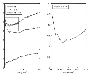
reported in Fig. 3 with λ = 1, evidencing that the “optimum” cardinality |Ω|∗= arg min|Ω|C obtained
0 0.05 0.1 0 2 4 6 8 10 12 14 card(!)/N2 0 0.01 0.02 0.03 0.04 8 8.5 9 9.5 10 10.5 11 card(!)/N2 H TV H + TV H + TV
Figure 3: Quantitative selection of the optimal cardinality |Ω| — Whereas the Shannon entropy (H) can measure TF localization, the Total Variation (TV) is proposed to be used as a penalty function for spiky solutions. A combination of both criteria (left panel, with an enlargement of the box in the right panel) turns out to attain its minimum value for a cardinality of the AF support that is in good agreement with
the “optimum” cardinality |Ω|∗ suggested by the oracle approach in Fig. 2.
3.3
On geometric adaptivity
It has been stressed that the selection of the Fourier samples in the AF domain deserved special attention in terms of area, but the question of it shape could be addressed as well. At first sight, it might be expected that the use of adapted kernels (as proposed, e.g., in [7]) would prove useful. This however seems not to be the case, which does not necessarily comes as a surprise. Indeed, besides an assumed sparsity of the solution, the other ingredient for a successful CS-based approach is that of its incoherence with the measurements on which it is based. Operating in the Fourier domain clearly goes this way, but adapting the selected subset to the signal structure goes the opposite.
References
[1] P. Borgnat and P. Flandrin, “Time-frequency localization from sparsity constraints,” in Proc. IEEE Int. Conf. on Acoust., Speech and Signal Proc. ICASSP-08, pp. 3785–3788, Las Vegas (NV), 2008. [2] E. Cand`es, J. Romberg and T. Tao, “Robust uncertainty principles: Exact signal reconstruction from
highly incomplete frequency information,” IEEE Trans. on Info. Theory, Vol. 52, No. 2, pp. 489–509, 2006. (see also http://www.dsp.ece.rice.edu/cs/ for a comprehensive resources page.)
[3] P. Flandrin, Time-Frequency/Time-Scale Analysis. San Diego: Academic Press, 1999.
[4] P. Flandrin, “Some features of time-frequency representations of multicomponent signals,” in Proc. IEEE Int. Conf. on Acoust., Speech and Signal Proc. ICASSP-84, pp. 41B.4.1–41B.4.4, San Diego (CA), 1984.
[5] P. Flandrin, F. Hlawatsch, “Signal representations geometry and catastrophes in the time-frequency plane,” Proc. 1st IMA Int. Conf. on Math. in Signal Proc., Bath (UK), 1985. Also in Mathematics in Signal Processing (T.S. Durrani et al., eds.), pp. 3–14, Clarendon Press, Oxford, 1988.
[6] F. Hlawatsch, P. Flandrin, “The interference structure of Wigner distribution and related time-frequency representations,” in The Wigner Distribution — Theory and Applications in Signal Pro-cessing (W. Mecklenbruker and F. Hlawatsch, eds.), pp. 59-133, Elsevier, Amsterdam, 1997.
[7] R.G. Baraniuk and D.L. Jones, “Signal-dependent time-frequency analysis using a radially Gaussian kernel,” Signal Proc., Vol. 32, No. 3, pp. 263–284, 1993.