HAL Id: tel-03108773
https://tel.archives-ouvertes.fr/tel-03108773
Submitted on 13 Jan 2021
HAL is a multi-disciplinary open access
archive for the deposit and dissemination of sci-entific research documents, whether they are pub-lished or not. The documents may come from teaching and research institutions in France or
L’archive ouverte pluridisciplinaire HAL, est destinée au dépôt et à la diffusion de documents scientifiques de niveau recherche, publiés ou non, émanant des établissements d’enseignement et de recherche français ou étrangers, des laboratoires
as tools for the history of science
Ian Jeantet
To cite this version:
Ian Jeantet. Hierarchical and temporal analysis of scientific corpora as tools for the history of science. Information Retrieval [cs.IR]. Université de Rennes 1 (UR1), 2021. English. �tel-03108773�
L’UNIVERSITÉ DE RENNES 1
ÉCOLE DOCTORALE NO601
Mathématiques et Sciences et Technologies de l’Information et de la Communication Spécialité : Informatique
Par
Ian JEANTET
Analyses hiérarchiques et temporelles de corpora scientifiques
vues comme outils pour l’histoire des sciences
Thèse présentée et soutenue à Rennes, le 5 janvier 2021
Unité de recherche : Institut de Recherche en Informatique et Systèmes Aléatoires
Rapporteurs avant soutenance :
Pierre Gançarski Professeur des universités à l’Université de Strasbourg
Christine Largeron Professeure des universités à Université Jean Monnet de Saint-Étienne
Composition du Jury :
Président : Elisa Fromont Professeure des universités à l’Université de Rennes 1
Examinateurs : David Chavalarias Directeur de recherche à l’Institut des Systèmes Complexes - PIF Pierre Gançarski Professeur des universités à l’Université de Strasbourg
Christine Largeron Professeure des universités à Université Jean Monnet de Saint-Étienne Zoltan Miklos Maître de conférences à l’Université de Rennes 1
La philosophie des sciences est une branche de l’épistémologie qui s’intéresse aux fondements, méthodes et implications de la science. Les philosophes essaient de définir, d’expliquer et de justifier la science d’une manière philosophique, c’est-à-dire distinguer la science de la non-science, déterminer son but, définir une bonne explication ou une bonne justification. L’histoire des sciences est l’étude du développement de la science. Les historiens des sciences se sont consacrés à répondre à des questions sur ce qu’est la science, comment elle fonctionne et si elle présente des modèles et des tendances visible à grande échelle. Ce sont deux domaines étroitement liés qui fonctionnent souvent ensemble.
Historiquement, il existe trois grands modèles d’évolution et d’interaction entre une ou plusieurs théories scientifiques.
Le premier modèle, associé à Popper, considère que le progrès scientifique passe par une falsification de théories incorrectes et l’adoption à la place de théories qui se rapprochent progressivement de la vérité. La science évolue de manière linéaire par accumulation de faits. La physique d’Aristote était surclassé par la mécanique classique de Newton elle-même surclassé par la relativité d’Einstein, etc.
Le principal modèle challengeant celui de Popper et proposé par Kuhn ne voit pas la science comme un progrès linéaire mais séparée en cycles à deux phases, une phase de science «normale» et une phase de science «révolutionnaire». Si la première phase est une période calme évoluant de manière similaire à la vision de Popper, la seconde, dans laquelle de nouvelles théories basées sur de nouvelles hypothèses sont testées, marque la séparation entre paradigmes. Les paradigmes sont des structures dominantes de pensée et de pratiques et représentent des hypothèses entièrement différentes et incommensurables (non comparables) sur l’univers. Il ne reste que peu de chose du paradigme précédent lorsqu’un changement se produit.
Un autre modèle extrême, promu par Feyerabend, réfute l’existence de méthodologies cohérentes utilisées par tous les scientifiques à tout moment et a argumenté durement contre l’idée que la falsification a jamais été vraiment suivie dans l’histoire de la science. Il a défendu sa position en remarquant qu’en pratique, les scientifiques considèrent ar-bitrairement les théories comme exactes même si elles ont échoué à de nombreux tests.
science et non-science.
De nombreuses autres théories ont été proposées pour nuancer ces trois principaux modèles. Ils présentent différentes variations dans la représentation du changement scien-tifique, de la notion de progrès et de la relation entre théorie et vérité.
Quels que soient les moteurs d’évolution de la science, la méthode scientifique qui produit la science de nos jours nécessite de confronter les théories à la réalité par une validation empirique. Ces résultats sont présentés à la communauté dans des publica-tions évaluées par des pairs. L’analyse des articles scientifiques produits au sein d’un domaine apparaît donc comme un bon moyen de déterminer les théories en jeu et l’étude de l’évolution de ces publications pourrait donner un aperçu des processus d’évolution en jeu. Les pionniers de l’épistémologie quantitative ont essayé de fournir des outils au-tomatiques pour cartographier le paysage scientifique afin de permettre aux historiens des sciences de comprendre pleinement l’évolution de la science. Certains ont tenté de con-struire des cartes basées sur un index de citation des articles scientifiques et des travaux plus récents ont introduit les notions de phylomémie, carte de métro et flux de texte ten-tant de générer des structures l’évolution de la science en se basant directement sur une étude du contenu des articles. L’étude du texte en lui-même a permis une granularité plus fine dans les cartes produites. La récente promotion pour une science ouverte a conduit à la disponibilité de très grands corpus de publications scientifique ce qui nécessitent des méthodes d’exploration de données de pointe pour en extraire des modèles d’évolution.
Pour reconstruire automatiquement des structures évolutives, les scientifiques doivent combiner plusieurs outils de traitement du langage naturel et d’exploration de texte suiv-ant une méthodologie divisée en plusieurs étapes et pouvsuiv-ant être définie comme suit :
— Récupération de données et répartition du corpus par périodes. Les périodes typ-iques pour étudier l’évolution récente de la science sont de quelques années, entre 3 et 5, avec une fenêtre glissante sur les périodes pour avoir un chevauchement des données. Comme la science évolue continuellement, diviser les données par périodes est arbitraire et avoir une division au milieu d’un événement particulier pourrait le rendre non détecté. Le chevauchement est là pour empêcher un tel comportement et identifier un maximum de ces événements.
— Extraction de termes et matrice de similarité. Cette étape transforme l’ensemble des documents de chaque période en une matrice de termes pondérée. Cette matrice vise à représenter la relation entre les termes clés, généralement des n-grammes.
mots dans un document.
— Détection des thématiques. Cela consiste à détecter des ensembles de termes forte-ment liés sémantiqueforte-ment dans des graphes de termes, la contrepartie graphique des matrices de co-occurrence.
— Correspondance inter-temporelle. Cela correspond à la mise en relation de do-maines de différentes périodes, généralement en utilisant l’index de Jaccard, pour en générer des lignes d’évolution temporelle. Cela conduira à des scissions dans les structures, similaires à celles présentes dans une structure phylogénétique, mais aussi à des fusions et d’autres événements spécifiques à ce type de carte évolutive. En général, une interaction avec la carte permet aux experts de personnaliser sa génération en modifiant les données (par exemple en supprimant ou en ajoutant un terme dans un domaine) ou les paramètres (par exemple en changeant l’intervalle de temps pour diviser le corpus de documents).
Les travaux présentés dans cette thèse visent à fournir une analyse automatique des publications scientifiques pour l’épistémologie quantitative. Comme plusieurs autres méth-odes, l’objectif final est de produire des cartes d’évolution des domaines scientifiques pour aider les épistémologues à déterminer les mécanismes en jeu et ce à partir du texte brut des publications.
Nous proposons d’abord d’enrichir les connaissances sur les relations existantes en-tre domaines scientifiques avec la définition d’une nouvelle structure hiérarchique appelée quasi-dendrogramme. Cette structure, une généralisation du simple arbre, peut être vue comme un graphe acyclique dirigé spécifique. Nous proposons un cadre d’étude com-prenant un nouvel algorithme de regroupement hiérarchique chevauchant (OHC) afin de générer une telle hiérarchie à partir d’un ensemble d’articles scientifiques. De cette façon, à chaque niveau, nous représentons un ensemble de regroupements éventuellement super-posés. Si les groupes présents dans les données ne montrent aucun chevauchement, ils sont alors identiques à des regroupements que nous pouvons déterminer en utilisant des méthodes de regroupement agglomératives classiques. Cependant, en cas de chevauche-ment et de groupes imbriqués notre méthode aboutit à une représentation plus riche qui peut contenir des informations pertinentes sur la structure entre ces groupes. En fait, cet algorithme peut être appliqué à tout autre type de données sur lequel une mesure de similarité est définie, exactement comme pour toute méthode de regroupement ag-glomérative. Par construction, nous avons prouvé des propriétés théoriques intrinsèques
données synthétiques et réelles, soulevant le problème de passage à l’échelle inhérent à ce type d’algorithme.
L’un des problèmes majeurs était également l’absence de jeu de données contenant une vérité terrain sur la structure de la science. Nous nous sommes retrouvés dans l’incapacité de comparer les hiérarchies que nous avons produites à de tels standards. Nous avons plutôt opté pour la définition d’une mesure de similarité afin de pouvoir comparer les quasi-dendrogrammes entre eux mais aussi avec d’autres structures hiérarchiques clas-siques comme les simples dendrogrammes. Nous voulions pouvoir mettre en évidence les spécificités et les régularités qui pouvaient se produire dans un ensemble de hiérarchies générées avec des algorithmes différents ou avec des paramètres différents sur un même jeu de données. À notre connaissance, très peu de travaux ont été effectués dans ce sens dans la littérature scientifique lorsque la structure devient plus complexe qu’un simple arbre. Nous avons donc proposé une nouvelle mesure de similarité qui aborde le problème par niveau. En effet, si pour deux structures hiérarchiques lorsque nous extrayons une couverture de k regroupements nous obtenons des groupes similaires pour toute valeur de k cela signifie que les structures sont très similaires et inversement. Nous avons util-isé cette mesure de similarité pour confirmer par l’expérience que l’algorithme OHC agit comme un algorithme à liaison simple classique lorsque le critère de fusion est proche de 1 et diffère de plus en plus lorsqu’il diminue. Nous avons également proposé une vue détaillée de la similarité pour détecter les parties communes et différentes des hiérarchies et une variante pondérée dans le but de réduire l’impact causé par les petits groupes agissant comme du bruit qui persisteraient dans les haut niveaux des hiérarchies. En fait, la détection de parties communes à plusieurs hiérarchies, c’est-à-dire qui sont produites pour plusieurs critères de fusion, peut être considérée comme un critère de robustesse.
Enfin, nous proposons une méthode alternative pour générer des cartes évolutives de domaines scientifiques à partir d’une requête d’un utilisateur sous la forme d’ensembles de termes représentant des sujets que l’utilisateur souhaite suivre. Dans notre cadre d’étude, une carte évolutive est définie comme un ensemble de chronologies, une chronologie étant une séquence de plusieurs groupes appartenant à des hiérarchies de périodes consécutives. Elles sont générées en utilisant des matrices d’alignement entre les hiérarchies. Nous pro-posons en détail une méthodologie complète permettant cette reconstruction et appliquons notre proposition à des quasi-dendrogrammes alignés à l’aide d’un algorithme spécifique. Nous avons également défini une probabilité d’évolution qui, si elle est utilisée comme
pruntées seront conservées. En bref cette nouvelle méthode peut être résumée comme suit :
— Récupération de données et répartition du corpus par périodes. Tout comme pour la méthodologie générale, le jeu de données est divisé en périodes plusieurs an-nées,ventre 3 et 5, se chevauchant pour lisser l’évolution et détecter le plus d’événements possible.
— Extraction de termes et plongements de mots. A cette étape, un ensemble de mots-clés est déterminé à partir des publications de chaque période. Ensuite, ils sont projetés dans un espace de grande dimension, un pour chaque période, en utilisant des techniques de plongement des plus avancées de la littérature.
— Détection de domaines. Cette partie est vraiment originale car elle consiste à déter-miner une structure hiérarchique des mots-clés avec possibilité de chevauchements entre les groupes de termes. Il en résulte la génération de quasi-dendrogrammes. — Correspondance inter-temporelle. Les cartes évolutives sont également le résultat
d’une nouvelle méthode. Ils sont produits à partir de requête d’utilisateurs en utilisant l’alignement d’un ensemble de quasi-dendrogrammes successifs.
Nous avons également créé des cahiers Jupyter interactifs qui permettent de générer des quasi-dendrogrammes et des cartes évolutives personnalisés. En fait, ils visent à fournir de l’interactivité pendant le processus de génération. Ils seront déposés sur un dépot git ainsi que le code qui sera open source.
L’un des principaux problèmes de cette nouvelle méthodologie de construction de carte évolutive est son évaluation. En effet, il est vraiment difficile de déterminer les propriétés générales ou les caractéristiques que toute carte évolutive devrait respecter. Comme pour les autres méthodes, la partie évaluation est laissée à l’expert et la qualité des cartes est basée sur des propriétés de construction propres à la méthode. Ainsi, un travail futur qui devrait être fait est une comparaison appropriée avec d’autres types de carte évolutive. Cela signifie déterminer une méthodologie standard dans lequel toutes les méthodes pourraient s’intégrer et proposer des évaluations pertinentes basées sur cette méthodologie. C’est délicat car toutes les cartes n’ont pas le même but et ne cherchent pas à montrer la même chose.
Aussi pour améliorer la méthode proposée qui utilise de nombreux outils à différentes étapes, tous autant importants, une étude approfondie peut être menée pour bien identifier les impacts des choix effectués pour construire les cartes évolutives et trouver le meilleur
philosophes des sciences. A cet effet, une interaction avec l’utilisateur apparaît également nécessaire pour analyser les structures produites et des outils de navigation interactifs semblent indispensables à court terme. En particulier il serait bien de pouvoir zoomer et dézoomer sur la structure de la science en se déplaçant plus haut ou plus bas dans les hiérarchies.
Je voudrais tout d’abord remercier mes deux encadrants Zoltan Miklos et David Gross-Amblard pour leur implication tout au long de cette thèse et notamment pour leurs précieux conseils de relecture.
Je remercie également Pierre Gançarski et Christine Largeron pour avoir accepté d’être les rapporteurs de ma thèse et d’avoir pris de leur temps pour apporter des remarques détaillées et constructives sur ces travaux.
Je tiens à remercier David Chavalarias et Elisa Fromont pour avoir fait parti de mon comité de suivi et avoir accepté de participer à mon jury de thèse.
Merci aussi à toutes les personnes avec qui j’ai pu travailler et échanger pendant ces trois ans, notamment mes collègues de l’équipe Druid.
Introduction 15
Context and motivation . . . 15
Main challenges and problem presentation . . . 16
Contributions . . . 18
1 State of the art 21 1.1 Text analysis . . . 21
1.1.1 Text preprocessing . . . 21
1.1.2 Keyword extraction . . . 25
1.1.3 Word embedding . . . 31
1.2 Hierarchical clustering . . . 43
1.2.1 Hierarchical agglomerative clustering (HAC) . . . 45
1.2.2 Density-based clustering . . . 49 1.2.3 Graph-based clustering . . . 52 1.2.4 Overlapping clustering . . . 53 1.2.5 Clustering evaluation . . . 55 1.3 Evolutionary structures . . . 58 1.3.1 Co-citation network . . . 59 1.3.2 Language evolution . . . 59 1.3.3 TextFlow . . . 60 1.3.4 Metro map . . . 60 1.3.5 Phylomemetic structure . . . 61
2 Overlapping Hierarchical Clustering (OHC) 63 2.1 Introduction . . . 63
2.2 From text to embeddings . . . 64
2.2.1 Text formatting . . . 64
2.2.2 Word embedding . . . 66
2.3.1 δ-neighbourhood . . . 71
2.3.2 Distance in high-dimensional space . . . 72
2.3.3 Graph density . . . 74
2.3.4 Quasi-dendrogram . . . 75
2.4 Overlapping Hierarchical Clustering (OHC) algorithm . . . 76
2.5 Properties of the algorithm . . . 77
2.6 Analysis . . . 79
2.6.1 Experimental setup . . . 79
2.6.2 Expressiveness . . . 80
2.6.3 Flat cluster extraction . . . 81
2.6.4 Time complexity of the OHC algorithm . . . 83
2.6.5 Optimisation . . . 85
2.7 Conclusion . . . 86
2.8 Detailed figures and tables related to the OHC algorithm . . . 87
3 Hierarchical structure similarity 97 3.1 Introduction . . . 97
3.2 Definition of the similarity measure . . . 97
3.2.1 Level similarity . . . 98
3.2.2 Global similarity . . . 98
3.3 Comparison of hierarchical structures . . . 100
3.4 Analysis and possible variants . . . 101
3.4.1 Detailed similarity . . . 101
3.4.2 Average versus weighted similarity . . . 103
3.5 Similarity as a search algorithm . . . 104
3.6 Conclusion . . . 105
4 Temporal analysis of hierarchical structures 107 4.1 Introduction . . . 107
4.2 Objectives and framework . . . 107
4.3 Evolutionary map . . . 109
4.4 Temporal matching . . . 110
4.4.1 Embedding alignment . . . 110
4.4.2 Hierarchy alignment principle . . . 114
4.5.1 Simple evolutionary map . . . 115
4.5.2 Complex evolutionary map . . . 118
4.6 Conclusion . . . 119
4.7 Detailed figures related to the evolutionary maps . . . 121
Conclusion 127 Results overview . . . 127
Future work . . . 129
Context and motivation
Epistemologists would like to understand the evolution of science and knowledge in general. If an expert relatively knows a bit of history and evolution of its own specific field, it becomes impossible to have an historical knowledge of wide scientific domains. Moreover, now with the hyper-specialisation of the scientific domains and the multiplication of the theories and axes of research, no one can pretend to be able to follow the evolutionary mechanisms that are at stake. This requires an automatic method to extract and analyse leading theories of scientific fields.
Historically there have been three major models of evolution and change between one or more scientific theories.
The first major model, associated to Popper’s view, considers that scientific progress is achieved through a falsification of incorrect theories and the adoption instead of theories which are progressively closer to truth. Science evolves in a linear fashion by accumulation of facts. The physics of Aristotle was subsumed by the classical mechanics of Newton subsumed itself by the relativity of Einstein, etc.
The main challenging model, proposed by Kuhn, sees science not as a linear progress but separated in two-phase cycles, "normal" science and "revolutionary" science. If the first phase is a calm period evolving similarly to Popper’s view, the second, in which new theories based on new assumptions are tested, marks the separation between paradigms. Paradigms are dominant structures of thought and practices and represent entirely differ-ent and incommensurate (non comparable) assumptions about the universe. Only little remains from the previous paradigm when a shift occurs.
Another extreme model, promoted by Feyerabend, refutes the existence of consistent methodologies used by all scientists at all times and argued harshly against the notion that falsification was ever truly followed in the history of science. He defended his position by noticing that in practice scientists arbitrarily consider theories to be accurate even if they failed many sets of tests. The same appears for some forms of knowledge that are
considered in turn as science and non-science.
Figure 1: Three models of change in scien-tific theories, depicted graphically to reflect roughly the different views associated with Karl Popper, Thomas Kuhn, and Paul Fey-erabend. CC BY-SA 3.01
Many other theories have been pro-posed to nuance these tree main models. They come with different variations in the representation of scientific change, the no-tion of progress and the relano-tion between theory and truth.
No matter the driving forces behind sci-ence evolution, the scientific method that produces science nowadays requires to con-front theories to the reality by empirical validation. These results are presented to the community through peer reviewed pub-lications. Hence analysing the scientific pa-pers produced by a domain appears to be good way to determine the theories in-volved and studying the evolution of these publications could give an access to the processes of evolutions.
Main challenges and
prob-lem presentation
Pioneers in quantitative epistemology tried to provide automatic tools to map the scientific landscape to allow historians of science to fully understand the evolution of science. Firsts tried to build maps based on citation index when more recent works got down to the study of the text itself which allowed a thinner granularity in the maps produced. The recent promotion for open science lead to the availability of massive
extract patterns from these large databases such as Wiley, dblp or Web of Science that gather millions of scientific publications.
To automatically reconstruct evolutionary structures, scientists need to combine sev-eral tools of Natural Language Processing and Text Mining in a workflow that can be divided in several steps and that is generally defined as follow:
— Data Retrieval and corpus splitting by periods. Typical periods to study recent evolution of science are several years, between 3 and 5, with a sliding window over the periods to have an overlap on the data. As science evolves continuously, splitting the data by periods is arbitrary and having a split in the middle of a particular event could make it undetected in the phylomemy, the overlap is here to prevent such behaviour.
— Term extraction and similarity matrix. This step transforms the set of documents of each period into a weighted term matrix. This matrix aims to represent the relationship between key terms, typically n-grams. The classical representation of this relationship is based on the co-occurrence of the words in a document.
— Topic detection. It consists in detecting sets of strongly semantically related terms within term graphs, the graphical counterpart of the term matrices.
— Inter-temporal matching. It matches topics from different periods, usually by using Jaccard index, to generate alignments representing the temporal evolution of the topics. This will lead to splits in the structures, which are common in a phyloge-netic structure, but also to merges and other typical events specific to this type of evolutionary map. Usually an interaction with the map allows experts to cus-tomize the workflow by changing data (for example removing or adding a term in a topic) and parameters (for example the time interval for dividing the document collection).
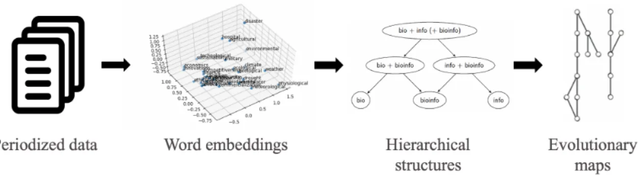
This is the main challenge of the ANR EPIQUE project, in which this thesis fits. Project partners have been pioneers in the reconstruction of science dynamics mining corpora at large scale (Chavalarias and Cointet 2013) and they have shown that we can characterize quantitatively the different phases of the evolution of scientific fields and automatically build “phylomemetic” topic lattices representing this evolution (Figure 2). Phylomemetic lattice comes as an analogy with the well known phylogenetic tree of natural species.
The project also involve philosophers of science, who perceive phylomemetic lattice structures as a tool for testing general accounts of progress and change in science. They
Figure 2: An existing workflow of phylomemy reconstruction (Chavalarias and Cointet 2013).
will play a role in validating the lattices produced in the context of the project. They especially underlined the necessity to map not only the evolution of scientific fields but also the global structure of science.
Contributions
In this thesis we propose an alternative workflow of generating evolutionary maps of scientific domains using state of the art techniques. It will allow to have different views on the structure of Science which constitutes interesting new tools for philosophers and historians of Science.
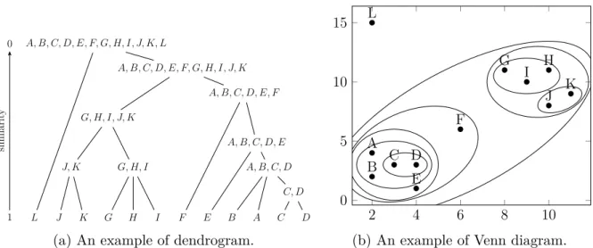
In the framework of analysing only the raw text of the scientific papers and not the citation index, a possible approach is to construct a word embedding of the key terms in publications, that is, to map terms into a high-dimensional space such that terms frequently used in the same context appear close together in this space (Section 1.1.3). Identifying for example the denser regions in this space directly leads to insights on the key terms of Science. Moreover, building a dendrogram of key terms using an agglomerative method is typically used (Chavalarias and Cointet 2013; Dias et al. 2018) to organize terms into hierarchies (Section 1.2). This dendrogram (Figure 3a) eases data exploration and is understandable even for non-specialists of data science.
Despite its usefulness, the dendrogram structure might be limiting. Indeed, any embed-ding of key terms has a limited precision, and key terms proximity is a debatable question. For example, in Figure 3a, we can see that the bioinformatics key term is almost equally attracted by biology and computing, meaning that these terms appear frequently together, but in different contexts (e.g. different scientific conferences). Unfortunately, with classical agglomerative clustering, a merging decision has to be made, even if the advantage of one
biology ∪ computing ∪ bioinformatics
biology ∪ bioinformatics
biology bioinformatics computing 0
1
distance
(a) A classical dendrogram, hiding the early relationship between bioinformatics and computing.
biology ∪ computing ∪ bioinformatics
bio ∪ bioinfo bioinfo ∪ computing
biology bioinformatics computing 0
1
distance
(b) A quasi-dendrogram, preserving the relationships of bioinformatics.
Figure 3: Dendrogram and quasi-dendrogram for the structure of Science.
cluster on another is very small. Let us suppose that arbitrarily, biology and
bioinformat-ics are merged. This may suggest to our analyst (not expert in computer science) that bioinformatics is part of biology, and its link to computing may only appear at the root
of the dendrogram. Clearly, an interesting part of information is lost in this process. The first contribution of this thesis is the proposition of a new Overlapping
Hierar-chical Clustering algorithm (Chapter 2) that combines the advantages of hierarchies
while avoiding early cluster merge. Going back to the previous example, we would like to provide two different clusters showing that bioinformatics is close both to biology and
computing. At a larger level of granularity, these clusters will still collapse, showing that
these terms belong to a broader community. This way, we deviate from the strict notion of trees, and produce a directed acyclic graph that we call a quasi-dendrogram (Figure 3b).
Figure 4: New workflow of evolutionary maps reconstruction.
For this purpose we define a density-based merging condition to identify these clusters. The second contribution is the definition of a new similarity measure (Chapter 3) to compare our method with other, quasi-dendrogram or tree-based ones. With this similarity measure and its variants we show through extensive experiments on real and synthetic data that we obtain high quality results with respect to classical hierarchical clustering, with reasonable time and space complexity.
Finally to complete the new workflow (Figure 4) the third contribution is the gen-eration of evolutionary maps (Chapter 4) as the result of the inter temporal study of the quasi-dendrograms. We produce these evolutionary maps based on queries made from an expert to interact with the flow of evolution of topics of science determined by quasi-dendrogram alignments.
The results presented in this thesis have been published in the following venues: — Ian Jeantet (2018), « Study science evolution by using word embedding to build
phylomemetic structures », in: BDA - Conférence sur la Gestion de Données –
Principes, Technologies et Applications. [PhD paper]
— Bernd Amann, David Chavalarias, Ian Jeantet, Thibault Racovski (2019), « Digital history and philosophy of science: The reconstruction of scientific phylomemies as a tool for the study of the life sciences », in: International Society for the History,
Philosophy and Social Studies of Biology meeting [Workshop]
— Ian Jeantet, Zoltán Miklós, and David Gross-Amblard (2020), « Overlapping Hi-erarchical Clustering (OHC) », in: International Symposium on Intelligent Data
Analysis, Springer, pp. 261–273. [Regular paper]
— Ian Jeantet, Thanh Trung Huynhn, Zoltán Miklós, David Gross-Amblard and Hung Nguyen Quoc Viet, « Mapping the evolutionary history of scientific concepts ». [To be submitted]
S
TATE OF THE ART
This state or the art Chapter will present a wide range of possible methods that can be used at different steps of the workflow. Even if the contributions are not at this part, we need to have an overview or the techniques of Natural Language Processing that allow to extract and represent information from a text, basically key terms and their relationships. Then we will see several techniques of clustering and their field of application that could determine topics among the keyterms. We will challenge these clustering techniques with our overlapping hierarchical clustering algorithm detailed later in Chapter 2. Also we will present classical evaluation techniques to see if they can or cannot be applied to our OHC algorithm. This will be explored in Chapter 3. Finally we will look at more general methods that already produce evolutionary maps to see on how the point of views and insights they allow are different from the one we propose in Chapter 4.
1.1
Text analysis
This first Section will explore state of the art methods that one can use in the two first steps of the evolutionary map reconstruction that is to determine key terms in a text, scientific publication in our scenario, then how to determine the relationship between terms. Also before that we need to explore the methods that need to be used to make a text readable to a machine.
1.1.1
Text preprocessing
Following the good practices given by Dias et al. 2018, in this section we discuss the possibilities of text reprocessing to transform text in human language from scientific papers to a machine readable format.
Language selection
First it seems logic that one need to select articles written in only one language. Nowadays as most of the them are written in English it is the obvious language to select to study recent datasets. It is also the most studied language hence the tools represented later will be more efficient on English terms. However for a specific study, especially on older datasets, another language could be considered.
Text selection
For most of available datasets one still don’t have access to the real content of the ar-ticles for copyright reason but to the title and optionally their abstract. For need as much text as possible so the title and abstract are concatenated for each article and considered as a unique entry.
From the raw text as a unique string we need to identify the words it contains and give them the correct form. It can be done in several ways.
Text cleaning
Apart from the words, a text contains many other characters that give a specific format to the text depending on the grammar of the considered language.
If it greatly eases the understanding of a text by a human reader, it only complexifies the work of an algorithm. Hence the following methods can be applied to uniform the words of a text. First one can simply convert all letters to lower (or upper) case. Then the numbers can be converted into words or be removed if they are not relevant for the study. Also contractions such as it’s can be replaced by their non-contracted form, it is in our example. A list based on Wikipedia’s List of English contractions1 is provided by Dias
et al. 2018. Finally punctuation and whitespaces, hidden characters such as tabulations ’\t’ or line breaks ’\n’ that represent a horizontal or vertical space and aerate the text, can optionally be removed. One must be careful that punctuation is essential for the comprehension of a text and cannot be removed for certain tasks.
Tokenization
One of the key steps is tokenization. Tokenization is the process of splitting a sequence of characters into a sequence of small pieces called tokens. Words and numbers, i.e. al-phanumeric chunks, are typical tokens but punctuation and white spaces can be consider as such and be included in the resulting list of tokens. Tokens can also mix letters and special characters such as hyphen depending on the rules that are applied for the tok-enization. The result of the tokenization depends on the cleaning done on the text and will differ if the punctuation was removed prior the tokenization for instance.
Having a list of tokens is enough to be use by a machine for further processing but depending on the task to perform, one needs to use more advance techniques that can help to improve the outcomes.
Token canonicalization
Language is composed of words that can take many inflected forms. For tasks like sorting documents into different categories, it is interesting to reduce them to their root or stem form. Indeed in this case the subtleties that exist between the word variants are not important.
Stemming In linguistic stemming is the process of reducing a word to its stem form. For example the words plants, planting and plantation should be reduce to the root form
plant. It is important to notice that a stem is not necessary a valid word as it is often the
result of the pruning of known suffixes and prefixes. For instance the word natural can be reduced to the stem natur.
Stemming algorithms have been studied since the 1960s and the main two stemmers are the Porter stemming algorithm extended to the Snowball stemmer family (Porter 2001) and the Lancaster stemming algorithm also known as the Paice-Husk Stemmer (Paice 1990). The second one is recognized to be a ’stronger’ stemmer, that is pruning more harshly the words, with its standard tuning, i.e. not changing any parameter.
Lemmatization In linguistic lemmatization is the process of identifying the canonical form (also called lemma) of a inflected word based on its meaning. Unlike stemming, lemmatization needs the context of a word to correctly identify the meaning of this word. The context is based on determining the part of speech of the word but can be extended
up to surrounding sentences and even the entire document. Common parts of speech of Indo-European languages are noun, verb, adjective, etc.
As examples:
— The word good is the lemma of the word better. This transformation is missed by a stemming algorithm.
— The word plant is the lemma of the word planted which is also identified by stem-ming.
— The word meeting can be either used as a noun of a verb and depending on the case the lemma is different, meeting for the noun and meet for the verb. While a stemmer will always select meet, lemmatization will try to identify the correct form based on the context.
Due to its complexity, finding an efficient lemmatization algorithm is still an open research area. Early works were mostly based on statistical models using an hand-build set of possible word-lemma pairs (Hakkani-Tür, Oflazer, and Tür 2002) when recent works are based on log-linear models (Müller et al. 2015) or neural networks (Bergmanis and Goldwater 2018; Bojanowski et al. 2017).
Then if stemmers are usually easier to implement and faster because based on rules they could be seen as less ’accurate’ than lemmatization algorithms. In fact in information retrieval tasks they reduce the precision, i.e. the capacity to detect only relevant infor-mation, and increase the recall, i.e. the capacity to detect all the relevant information (Christopher D. Manning, Raghavan, and Schütze 2009).
Also for other tasks such as finding the relationship between words for syntactic or semantic reason it is not possible to perform stemming or lemmatization because we need to preserve the relationship between every inflected word forms, between good, better and
best for instance.
Token cleaning
Finally, non interesting tokens can be removed from the text. Usually one remove single character tokens that often come from a bad detection during the tokenization process and that are non word tokens.
At this step it is also possible to remove numbers and/or stop word tokens. Stop words are extremely common words that appear to have little value in tasks like information retrieval or search engine query and hence that can be discarded to decrease the size of
the dataset and improve the performances and accuracy. Indeed, a keyword search based on words like the or from is not really useful. However the trend is to include them as much as possible and for other tasks like phrase search or machine translation they are at upmost importance and should be preserved. For example, this movie is not good has a different and more precise meaning than the isolated words movie and good.
There is no universal stop word list. To be not significant, a word needs to be evenly distributed in a collection of texts. Indeed if it appears with the same frequency in all the texts it cannot be used to discriminate and select specific ones in the collection. If all the texts are in the same language these words are usually function words like the,
at, which, etc for English and combination of existing lists are often used. However for
a corpus of texts on a common theme, specific words can be uniformly distributed and then should be also considered as stop words and on the contrary some function words appear rarely in texts. Another practical approach (Christopher D. Manning, Raghavan, and Schütze 2009) consists in ordering the words by collection frequency, i.e. considering the total number of occurrence of each word in all the texts, and taking the list of most frequent words as stop words.
1.1.2
Keyword extraction
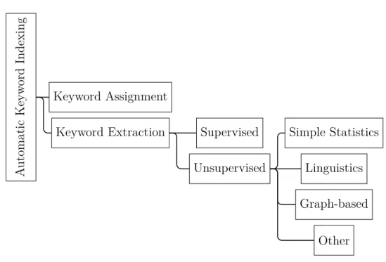
Keywords are important terms and phrases within documents. They play an important role in many applications in Text Mining, Information Retrieval and Natural Language Processing and also in our workflow. With the huge quantity of documents now available it is illusory to think of being able to read them all and find information in them. For this reason it is mandatory to have an automatic approach. In keyword assignment, the key-words are chosen from a predetermined set of terms that match the most the documents. In this section we will see methods of keyword extraction that is to extract the keywords directly from the documents, as it corresponds to the task we will need to perform on scientific publications, and we will discuss the great diversity of these approaches (Figure 1.1).
Statistical approaches
Methods using statistical rules are among the simplest to detect keywords or key phrases as they don’t require prior knowledge either on the domain or the language. However they are based on rules and hence can miss specific relevant keywords.
A utomatic Keyw ord Indexing Keyword Assignment
Keyword Extraction Supervised
Unsupervised Linguistics
Simple Statistics
Graph-based
Other
Figure 1.1: Classification of keywords extraction methods (adapted from Beliga, Meštro-vić, and Martinčić-Ipšić 2015).
Word frequency Sorting words by frequency allows to detect words that appear com-monly in a text or corpus. It is useful to determine the main theme of a document or the most common issues from a Q&A section for instance.
However this approach consider text as a bag-of-words (Definition 1) putting com-pletely aside the meaning of the words and the structure of the text.
Definition 1 (Bag-of-words model, Harris 1954). The bag-of-words model is used in NLP
and IR as a simplification of text representation. In this model a text is represented as the multiset (the bag) of its words that is by keeping only the words and their multiplicity, excluding grammar like punctuation and even the word order.
Hence this method will also detect frequent language-specific function words and miss synonyms, dismissing valuable information.
N-grams and word co-occurrences To understand better the semantic structure of a text, one can use statistics to detect words that appear frequently together. In this case they can be considered as a unique entity which allows to extract more complex terms from the documents.
It can be frequent adjacent words in the case of word n-grams (Definition 2). The sequence new york times can be composed of 3 separated words but one can also consider
the bi-gram new york which refers to the city, keeping times aside, or the tri-gram new
york times which refers to the journal. In each of these cases, one can see that the meaning
of the words radically changes which implies a different understanding of the text.
Definition 2 (gram). In the fields of computational linguistics and probability, an
n-gram is a contiguous sequence of n items from a given sample of text or speech. The items
can be phonemes, syllables, letters, words or base pairs according to the application.2
In a corpus, statistics can also be used to detect words that frequently co-occur in the same texts without having to be adjacent. If the relation between the words is less direct, they still have a semantic proximity.
TF-IDF TF-IDF, that stands for term frequency–inverse document frequency, is a fam-ily of statistics that aims to measure how important a word is to a document in a corpus. TF-IDF is the product of two statistics, the term frequency and the inverse document
frequency. It exists various ways to determine these values.
The term frequency is the same measure as explained in the previous paragraphs. It counts the number of occurrence of a term in a document. If one wants to identify the documents that correspond the most to a query like the brown fox, relevant documents should be the documents where these three words have the most weight. Luhn 1957 first stated that the weight of a term that occurs in a document is proportional to the term frequency. If the raw count is the simplest choice, adjustments are often made to take the length of the documents into account for instance. In this case one can divide the raw frequency of a term t in a document d by the number of words in the documents (Equation 1.1).
tf (t, d) = P ft,d
t0∈dft0,d
(1.1) However for common terms such as the in our example the term frequency will tend to highlight documents that frequently contain this term without distinction with the two other terms that are more specific. To overcome this issue and give more weight to the terms that occur rarely, Jones 1972 introduced a term-specificity statistic called inverse
document frequency on the idea that the specificity can be quantify as an inverse function
of the number of documents in which it occurs. Classical inverse document frequency can be obtained by taking the logarithm of the inverse fraction of the number of documents
containing the term t by the total number of documents N = |D| of the corpus D (Equation 1.2). Similarly to the term frequency, it exists many variants for the inverse
document frequency.
idf (t, D) = log |D|
|{d ∈ D|t ∈ d}| (1.2)
As the product of the two measures (Equation 1.3), a high TF-IDF is reached when a term appears frequently in a document and, on the contrary, if this term appears in many documents, the ratio in the logarithmic function will be closer to 1 and hence the TF-IDF closer to 0.
tf –idf (t, d, D) = tf (t, d) · idf (t, D) (1.3)
Extracting keyterms based on this measure is interesting, they have a special meaning with regard to the corpus. In particular they are frequent in the documents but certainly not evenly distributed as they need to appear in less documents as possible. As an example, one of the state-of-the-art TF-IDF functions is the ranking function called Okapi BM25 (Robertson and Zaragoza 2009; Whissell and Clarke 2011).
Linguistic approaches
To improve statistical approaches one can use linguistic information about the texts and the words. In combination with a method seen above, one can use it to reduce a preselected set of keyterms.
This linguistic information can be the part-of-speech (PoS) of the words. One can give a higher score to nouns as they often carry more information than other type of words.
Also the position of a word in a text can give some information about its importance (X. Hu and Wu 2006). If a word appears in the first and last paragraphs of a document, usually the introduction and the conclusion, it is generally more important. Same for words of the leading and concluding sentences of a paragraph. Detecting conjunctions and discourse markers that connect expressions and sentences can also be used for this purpose. X. Hu and Wu 2006 stated that their method called Position Weight Inverse Position Weight (PWIPW) outperforms standard TF-IDF.
Graph-based approaches
A graph is defined as a set of vertices with some connections between them, the edges. A graph is a well established mathematical structure that facilitates an efficient exploration of the structure and the relationships between the vertices.
Graph generation They are many ways to represent a text as a graph. Usually the words are the vertices and the edges represent the relationship between the words but depending on the goal, different methods can use different linguistic units as vertices and the generated graph can be directed or undirected, weighted or unweighted. Beliga, Meštrović, and Martinčić-Ipšić 2015 and Firoozeh et al. 2020 gave an overview of the different principles on which the edges between the vertices of the graph can be established. — Co-occurrence graphs. They connect words co-occurring in a window of a given number of words in the text. This type of graphs are used in particular by TextRank-like algorithms (Mihalcea and Tarau 2004). They can also connect all the words of a sentence, paragraph, section or even document that hence will appear as a clique (Definition 11) in the graph.
— Syntax dependency graphs. They connect words according to the syntactic relation-ship of the part-of-speech they belong (Huang et al. 2006; Liu and F. Hu 2008). — Semantic-based graphs. They connect words that have similarities in their
mean-ing, spellmean-ing, that are synonyms, antonyms, homonyms, etc. For instance Grineva, Grinev, and Lizorkin 2009 exploit semantic relations of terms extracted from Wikipedia to built such graphs.
Graph analysis From such a graph, keyword extraction works by measuring how im-portant is a vertex to the graph, i.e. a word to the text, based on information given by the structure of the graph. Beliga, Meštrović, and Martinčić-Ipšić 2015 and Firoozeh et al. 2020 also presented several methods of the literature that serve this purpose. Unsuper-vised methods to get a list of keywords are divided into two main categories: clustering and ranking algorithms.
— Clustering algorithms. They work by grouping together nodes of the graph that are semantically related. For tasks such as indexing, Ohsawa, Benson, and Yachida 1998 showed that, with their KeyGraph algorithm, a clustering based on a co-occurrence graph outperforms TD-IDF and N-grams approaches. They also proved KeyGraph to be a content-sensitive and domain-independent indexing device.
An-other approach from Grineva, Grinev, and Lizorkin 2009 uses community detection techniques to identify relevant words and discard irrelevant ones.
— Ranking algorithms. This approach is the most common and aims at giving a rank to the vertices of the graph based on the global information represented by entire graph. The technique was introduced by Mihalcea and Tarau 2004 with their TextRank algorithm. They adapted the PageRank algorithm on a weighted co-occurrence graph and the result appeared as a strong baseline for this type of algorithms. It exists many other variants and an extensive presentation of them is given by Beliga, Meštrović, and Martinčić-Ipšić 2015.
Supervised approaches
One can see keyword extraction as a classification problem that aims to labelled each keyword candidates as either keyword or non-keyword. One of the first classifiers is the Keyphrase Extraction Algorithm (KEA) proposed by Frank et al. 1999. It uses a Naïve Bayes algorithm based on statistical and informational features for the training and it had many improvement over the years. It exists many other supervised methods that are presented in details by Firoozeh et al. 2020. One can notice the work of Krapivin et al. 2010 that uses NLP techniques to improve Machine Learning approaches for the automatic keyword extraction from scientific papers as it is closely related to the subject of this thesis. They showed that this outperforms the state-of-the-art KEA without the use of controlled vocabularies.
In general these supervised methods compete with unsupervised ones but the training data requirement is a strong limitation as it has to be generated manually which is very costly. Sterckx et al. 2016 pointed out the difficulty to find reliable training data which has consequences on the outcomes.
Discussion on the methods
According to Firoozeh et al. 2020, due to its difficulty Keyword Extraction is still an open area of research and there is no single efficient method that would work in all applications. Each one has its pros and cons with a F-measure around 50% for the highest reported scores in the literature. The F-measure is an accuracy measure that consider both the precision and the recall to compute its score. The precision is the capacity of a method to retrieve only relevant information, in our case relevant keywords, and the
recall is the capacity of a method to retrieve all relevant information. More details about
the F-measure are given in Section 1.2.5.
If a supervised approach can be a good choice when annotated data are available, for the vast majority when it’s not the case, unsupervised approaches are a better choice. Among them TF-IDF has been widely used and recent approaches combine it with other methods such as graph-based ones. Also TF-IDF can be comparable to such graph-based methods on specific cases. In fact TF-IDF tends to identify specific and representative words when graph-based methods also search for completeness.
It is also possible to remove irrelevant keywords afterwards using termhood processing. Similarly to the word frequency method the idea is to remove evenly distributed keyword candidates. It doesn’t matter if they are technical words or phrases, if they appear in all the documents they are considered neutral with respect to the given corpus (Chavalarias and Cointet 2013; Van Eck and Waltman 2011). If the corpus is related to a specific domain one can also asks to expert to finish the cleaning of irrelevant keywords (Chavalarias and Cointet 2013).
1.1.3
Word embedding
We explored methods useful to format a text and to extract keyterms from a corpus. Now we need a method that we can use to determine the meaning of the these terms and the relation it exists between them. It will be necessary for the second step of our workflow. Word embedding gives a standard representation of words or terms which serves this purpose. It is a general technique in Natural Language Processing (NLP) where words or phrases from a vocabulary are mapped to a high-dimensional vector space. It aims to quantify and categorize semantic similarities between language terms based on their distributional properties in large samples of data. For instance the word "kangaroo" will be more related to the word "Australia" than to other words such as "Russia" or "watermelon". We will see in this section a review of different possible methods of word embedding.
Co-occurrence based approaches
Traditionally in the literature a term is represented by the "bag of documents" in which the term occurs. This representation is the Document Occurrence Representation (DOR) where a term vector contains the document weights that correspond to the contribution of each document of the corpus to the semantic specification of the term. Latent Semantic
Analysis (Dumais 2004) uses this representation. The key steps of LSA are computing this term-document matrix, using typically TD-IDF as weights, and performing a dimension reduction using Singular Value Decomposition (Golub and Reinsch 1971) on this |T | × |D| matrix. The resulting k × k matrix is the best k-dimensional approximation of the original matrix using the least squares method. Now each term (and document) has a
k-dimensional vector representation.
As shown by Lavelli, Sebastiani, and Zanoli 2004, basic DOR is outperformed by a second approach, the Term Co-Occurrence Representation (TCOR) which differs from DOR by representing the terms as "bags of terms", i.e. vectors of term weights instead of document weights. As in DOR these weights correspond to the contribution of every term in the vocabulary to the semantic specification of the represented term. The classical |T | × |T | co-occurrence matrix is a typical example of the TCOR representation. The Hyperspace Analogue to Language (Lund and Burgess 1996) model also uses this term-term matrix representation. The cells of the matrix are updated according to the co-occurrence of terms in a 10 word window sliding over the text. The cell corresponding to the co-occurrence of two terms is increased by ∆ = 11 − d where d is the distance between the two terms in the window. One of the strength of the TCOR is to be "corpus independent" in the sense that the size of the matrix does not depend on the number of documents in the corpus.
Neural Network Language Models (NNLM)
The main power of neural network based language models is their simplicity. The same model with only few changes can be used for projection of many type of signals including language. Also these models performs implicitly clustering of word in low-dimensional space which gives us a robust and compact representation of words.
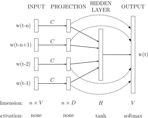
Among the first neural models used in NLP, Bengio, Ducharme, et al. 2003 proposed a probabilistic feedforward NNLM which consists of input, projection, hidden and output layers. The n previous words are represented as one-hot vectors (Definition 3) of size V where V is the size of the vocabulary. The input layer is projected to a projection layer P of a n × D dimension that uses a shared projection matrix noted C in Figure 1.2. Then these n projected vectors feed a hidden layer of a H dimension that use the hyperbolic tangent as activation function. Finally the hidden layer is used to compute the probability distribution over all the words in the vocabulary through a softmax activation function.
It results in an output vector of size V .
Q = n × D + n × D × H + H × V (1.4)
The computational complexity per training Q is as shown as in Equation 1.4 where the dominating term is H × V . However, as Tomáš Mikolov, K. Chen, et al. 2013 recall us, several alternatives are existing to go down the complexity to H × log2(V ). Hence the
dominating term becomes n × D × H.
Definition 3 (One-hot encoding). A one-hot vector is a 1×|V | matrix used to distinguish
each word in a vocabulary of size |V | from every other word. The vector consists of 0s in all cells with the exception of a single 1 in a cell used uniquely to identify the word.
INPUT PROJECTION HIDDEN
LAYER OUTPUT w(t-n) w(t-n+1) w(t-2) w(t-1) n × V dimension: none activation: n × D none H tanh V softmax w(t) C C C C
Figure 1.2: Neural architecture of the feedforward NNLM (adapted from Bengio, Ducharme, et al. 2003).
Language models using a recurrent neural networks (RNNLM) have been proposed by Bengio, LeCun, et al. 2007, Tomáš Mikolov, Karafiát, et al. 2010 and Tomáš Mikolov, Kombrink, et al. 2011. Unlike feedforward neural networks a RNN has no projection layer which means this model is independent to the specified order n of the feedforward NNLM. The architecture of the basic RNN model, also called Elman network, is shown in Figure
1.3. In RNN the model uses only the previous word as input but also a recurrent matrix (R in the figure 1.3) which contains the previous weights of the hidden layer. This re-current matrix and the input word represented by a one-hot vector are concatenated and connected to the hidden matrix H. It simulates a time delayed connection and represents some kind of short term memory. The same well known activation functions (sigmoid and softmax) are used in this model and the network is trained by using the standard back-propagation technique. After some optimisations mainly from Tomáš Mikolov, Kombrink, et al. 2011, the computational complexity per training is
Q = H × H + H × V (1.5)
As said previously for the feedforward NNLM, the term H × V in Equation 1.5 can be reduce to H × log2(V ) then most of the complexity comes from H × H.
INPUT HIDDEN
LAYER OUTPUT
R
H
w(t-1) w(t)
Figure 1.3: Simple recurrent neural network architecture.
Log-linear models
The main problem of the existing NNLMs is their computational complexity which is caused by a non-linear hidden layer in the models. This complexity is a real chal-lenging problem when it comes to deal with very large amount of training data and high-dimensionality of the word vectors. To reduce this complexity, Tomáš Mikolov, K. Chen, et al. 2013 proposed to use simpler model architectures: Continuous Bag-of-Words (CBOW) and Skip-gram models.
The goal of these two models is to tell us the probability for every word in our vo-cabulary of being the nearby word of a given word we chose. In Figure 1.5, nearby means 2 words behind or ahead from the position of the chosen word in the sentence. More generally we note this window size C as in Figure 1.4.
INPUT HIDDEN LAYER OUTPUT • • • wI1 • • • wI2 • • • wI3 • • • wIC C × V -dim • • D-dim • • • wO V -dim WV ×D WV ×D WV ×D WV ×D WD×V0 (a) CBOW INPUT HIDDEN LAYER OUTPUT • • • wO1 • • • wO2 • • • wO3 • • • wOC C × V -dim • • D-dim • • • wI V -dim WD×V0 WD×V0 WD×V0 WD×V0 WV ×D (b) Skip-gram
Figure 1.4: (a) The CBOW architecture predicts the current word based on the context when (b) the Skip-gram predicts surrounding words given the current word (adapted from Tomáš Mikolov, K. Chen, et al. 2013).
The word pairs as shown in Figure 1.5 will be used to train a neural network. At the third step (the third line of the figure) the words the, quick, fox and jumps will be inputs for the CBOW model when the expected output brown will be used for backpropagation learning. As the Skip-gram model works in mirror of the CBOW model, brown will be the input and the 4 other words the expected outputs. It is important to notice that
Source Text Training Samples
The quick brown fox jumps over the lazy dog. ⇒ (the, quick)
(the, brown)
The quick brown fox jumps over the lazy dog. ⇒
(quick, the) (quick, brown) (quick, fox)
The quick brown fox jumps over the lazy dog. ⇒
(brown, the) (brown, quick) (brown, fox) (brown, jumps)
The quick brown fox jumps over the lazy dog. ⇒
(fox, quick) (fox, brown) (fox, jumps) (fox, over)
Figure 1.5: Example of some of the word pairs taken from the sentence The quick brown
fox jumps over the lazy dog (adapted from McCormick 2016).
under the bag-of-words assumption, the order of the context words has no influence on the prediction.
Let see in details how the CBOW model works by looking at the forward propagation (how the output is computed from the inputs) and the backpropagation (how the weight matrices are trained).
For the forward propagation one assume that the input and output weight matrices are known, respectively noted W and W0 in Figure 1.4. The output of the hidden layer
h is the average of the sum of the inputs vectors weighted by the matrix W which is
formally expressed by h = 1 CW · C X i=1 wIi (1.6)
In fact the average vector of the inputs is projected on a space of dimension D. One can notice that in this model there is no activation function for the hidden layer. From the hidden layer to the output layer, using each column of the weight matrix W0 one can compute a score for each word of the vocabulary by calculating
uj = W∗,j0
T
where W∗,j0 is the j-th column of W0. uj is a measure of the match between the context
and the candidate target word. Finally the output wO is obtained from the output layer
by passing uj through the softmax function to calculate its j-th component.
wOj = p(wj|wI1, ..., wIC) =
exp(uj)
PV
j0=1exp(uj0)
(1.8) Each component represents the probability of the word wj of the vocabulary to be the
output word knowing the context so the output vector is in fact a probability distribution and not a one-hot vector.
Now let see how the weights of the two matrices are learnt. As said before, the word pairs as shown in Figure 1.5 are used to feed the model. The training objective is to match the probability distribution calculated by the model wO with the one-hot vector
representing the target word wT. To do this every distance could be used but the most
common one is the cross entropy.
Definition 4 (Cross entropy). Considering p and q two discrete probability distributions,
the cross entropy is defined as
E(p, q) = −X
x
p(x) log q(x) (1.9)
In this case as the target word is a one-hot vector, the distribution p in 1.9 is equal to zero except for the j-th component then
E(wT, wO) = − V X i=1 wTilog wOi = − log wOj = − log p(wj|wI1, ..., wIC) (1.10)
Finally using 1.7 and 1.8 one can define the loss function as
E(wT, wO) = − log p(wj|wI1, ..., wIC) = − logPVexp(uj) j0=1exp(uj0) = log V X j0=1 exp(uj0) − uj (1.11)
One way to minimize this loss function is to use the gradient descent technique or stochas-tic gradient descent (SGD) which allow to find a local minimum of a differentiable function or a sum of differentiable functions and then to reduce the error by updating the weight matrices accordingly.
Definition 5 (Gradient descent). It is a first-order iterative optimization algorithm for
finding the minimum of a differentiable function. To find a local minimum of a function using gradient descent, the idea is to move step by step in the direction of the negative gra-dient (or of the approximate gragra-dient) of the function at the current point. This technique works in spaces of any number of dimensions and even if it exists better alternatives this one stays computable for extremely large problems. Several extensions are also used such as the momentum method which reduces the risk of getting stuck in a local minimum.
The Skip-gram model (Figure 1.4) is the opposite of CBOW but the equations are very similar. This model uses the same matrices W and W0. As there is only one input word, for the Skip-gram model the output of the hidden layer is simply a projection of the word wI on a D-dimensional space using the weight matrix W and 1.7 becomes:
h = wI· W = Wk,∗ (1.12)
The difference now with CBOW is that one need to compute C probability distributions and not only one. All of these distributions will be computed using the same weight matrix
W0 as following: p(wOj|wI) = exp(uj) PV j0=1exp(uj0) (1.13) And then for the backpropagation, the loss function is changed to:
E = − log p(wO1, wO2, ..., wOC|wI) = − log C Y c=1 p(wOc|wI) (1.14)
Hence: E = − log C Y c=1 exp(uc,jc) PV j0=1exp(ui,j0) = C · log V X j0=1 exp(uj0) − C X c=1 ujc (1.15)
This equation is very similar to 1.11, the computed probability distribution needs to match with the C context words that are known during the training. The same technique of gradient descent is also used for backpropagation in the Skip-gram model.
These two models don’t seem to generate word vectors but here is the trick that Tomáš Mikolov, K. Chen, et al. 2013 used, after the training each line of the input matrix W will be in fact a very good representation of each words in a D-dimensional space. Indeed, if two different words have similar contexts, ie the same words appear around them, then the model needs to output very similar results. One way for the network to do this is to have similar word vectors for these two words. However as Goldberg and Levy 2014 argue, there is a strong hypothesis saying that words in similar contexts have similar meanings which should to be better defined even though as human we often use the context to determine the meaning of a new word.
Tomáš Mikolov, K. Chen, et al. 2013 compared these two models with the previous NNLMs (feedforward and recurrent) on semantic and syntactic questions. They concluded that, even with distributed frameworks to train the models, because of the much lower computational complexity it is possible to train the CBOW and Skip-gram models on several order of magnitude larger datasets than the other NNLMs. Thanks to this much better training CBOW and Skip-gram outperform more complex NNLMs on the tested NLP tasks with an advantage to the Skip-gram model which work well with "small" amount of training data and represent better rare words than the CBOW model which is several times faster to train and has a slightly better accuracy on frequent words.
Parametrization of the CBOW and Skip-gram models
With the objective to improve even more the Skip-gram model, Tomáš Mikolov, Sutskever, et al. 2013 proposed several useful additional techniques.