On the flutter bifurcation in laminar flows : linear and nonlinear modal methods

(1)

HAL Id: tel-03160958

https://tel.archives-ouvertes.fr/tel-03160958

Submitted on 5 Mar 2021

HAL is a multi-disciplinary open access archive for the deposit and dissemination of sci-entific research documents, whether they are pub-lished or not. The documents may come from teaching and research institutions in France or abroad, or from public or private research centers.

L’archive ouverte pluridisciplinaire HAL, est destinée au dépôt et à la diffusion de documents scientifiques de niveau recherche, publiés ou non, émanant des établissements d’enseignement et de recherche français ou étrangers, des laboratoires publics ou privés.

On the flutter bifurcation in laminar flows : linear and

nonlinear modal methods

Johann Moulin

To cite this version:

Johann Moulin. On the flutter bifurcation in laminar flows : linear and nonlinear modal methods. Fluid mechanics [physics.class-ph]. Institut Polytechnique de Paris, 2020. English. �NNT : 2020IP-PAX093�. �tel-03160958�

(2)

626

NNT

:2020IPP

AX093

On the flutter bifurcation in laminar flows:

_{linear and nonlinear modal methods}

Thèse de doctorat de l’Institut Polytechnique de Paris préparée à l’ École polytechnique École doctorale n◦₆₂₆

´Ecole Doctorale de l’Institut Polytechnique de Paris (ED IP Paris)

Spécialité de doctorat : Mécanique des fluides et des solides

Thèse présentée et soutenue à Meudon, le 7 décembre 2020, par

J

OHANN

M

OULIN

Composition du Jury : Jacques Magnaudet

Directeur de recherche, CNRS (Institut de M´ecanique des Fluides

de Toulouse) Pr´esident

Grigorios Dimitriadis

Professeur, Université de Liège (Département d’Aérospatiale et

M´ecanique) Rapporteur

Ardeshir Hanifi

Docent, KTH Royal Institute of Technology in Stockholm

(Department of Engineering Mechanics, FLOW Centre) Rapporteur Xavier Amandol`ese

Maˆıtre de conférences, Conservatoire National des Arts et Métiers (Laboratoire de Mécanique des Structures et des Systèmes

Coupl´es) Examinateur

Flavio Giannetti

Professeur associ´e, Universit`a degli Studi di Salerno (Dipartimento

di Ingegneria Industriale) Examinateur

Pierre Jolivet

Charg´e de recherche, CNRS (Institut de Recherche en Informatique

de Toulouse) Examinateur

Olivier Marquet

Maˆıtre de recherche, ONERA (D´epartement A´erodynamique,

Aéroélasticité, Acoustique) Directeur de thèse Denis Sipp

Directeur de recherche, ONERA (D´epartement A´erodynamique,

(3)

(4)

i

A

BSTRACT

The flutter instability has been the focus of numerous works since the middle of the twentieth century, due to its critical application in aeronautics. Flutter is classically described as a linear instability using potential flow models, but viscous and non-linear fluid effects may both crucially impact this aeroelastic phenomenon.

The first part of this thesis is devoted to the development of theoretical and nu-merical methods for analyzing the linear and nonlinear dynamics of a typical aeroe-lastic section — a heaving and pitching spring-mounted plate — immersed in a two-dimensional laminar flow modeled by the incompressible Navier–Stokes equations. A semi-analytical weakly nonlinear analysis (WNL) is first developed in order to de-rive an amplitude equation for the flutter bifurcation. In order to bypass the inherent limitations of this method to weak nonlinearities, we then develop a harmonic bal-ance type method, known as the Time Spectral Method (TSM), allowing to efficiently compute — possibly unstable — highly-nonlinear periodic flutter solutions. The challenging task of solving the TSM equations, especially when large numbers N of Fourier harmonics are considered, is tackled via a time-parallel Newton—Krylov approach in combination with a new, so-called block-circulant preconditioner, for which N-robustness is numerically demonstrated.

The second part of this thesis focuses on the physical investigation of the flut-ter bifurcation of the spring-mounted plate. We start by revisiting the linear stabil-ity problem using a Navier–Stokes fluid model allowing to highlight, in particular, the effect of viscosity. Comparisons to classical quasi-steady and unsteady poten-tial flow (Theodorsen model) theories are performed. Contrary to what happens in potential flows, the flutter instability is shown to re-stabilize at very high reduced velocities in viscous flows. We continue our route on the flutter bifurcation by vestigating the effect of fluid nonlinearities. Low solid-to-fluid mass ratios and in-creasing Reynolds numbers foster subcritical bifurcations. The role of leading-edge shear layers is pointed out. For intermediate mass ratios, an unusual bifurcation scenario that combines a supercritical bifurcation and the existence of subcritical high-amplitude flutter solutions is discovered. We conclude our study of the flutter bifurcation by investigating the appearance of low-frequency amplitude modula-tions on top of a previously established periodic flutter solution. Using an original TSM-based Floquet stability analysis, we explain this behavior by the destabilization of the periodic solutions by a pair of complex-conjugate Floquet modes. An analysis of the latter shows that the physical mechanism governing the instability borrows elements from the classical flutter instability arising on steady solutions.

The last part of this thesis aims at initiating the extension of the different methods previously evoked to large-scale three-dimensional configurations. As a first step to-wards this long-term goal, we develop an open-source massively parallel tool, based on the FreeFEM library and its PETSc/SLEPc interface, able to compute the nonlin-ear steady-state flow and subsequently solve the linnonlin-ear stability eigenproblem, for three-dimensional flows (the structure is fixed) possessing several tens of millions of degrees of freedom.

(5)

(6)

iii

R

ÉSUMÉ FRANÇAIS

L’instabilité de flottement a été le sujet de nombreuses études depuis le milieu du vingtième siècle à cause de ses applications critiques en aéronautique. Elle est clas-siquement décrite comme une instabilité linéaire en écoulement potentiel, mais les effets visqueux et nonlinéaires du fluide peuvent avoir un impact crucial.

La première partie de cette thèse est consacrée au développement de méthodes théoriques et numériques pour l’analyse linéaire et nonlinéaire de la dynamique d’une “section typique aéroélastique” — une plaque montée sur des ressorts de flexion et torsion — plongée dans un écoulement laminaire bidimensionnel mod-élisé par les équations de Navier–Stokes incompressibles. D’abord, on développe une analyse faiblement nonlinéaire afin d’établir une équation d’amplitude pour la bifurcation de flottement. Afin de dépasser la limitation aux faibles nonlinéar-ités (i.e. faibles amplitudes) inhérente à cette approche, on met en place ensuite une méthode de type équilibrage harmonique, connue comme la Méthode Spec-trale en Temps (TSM). Cette dernière permet de calculer efficacement des solutions périodiques de flottement plus fortement nonlinéaires et possiblement instables. Le défi de la résolution numérique des équations TSM, en particulier dans le cas où un grand nombre d’harmoniques est pris en compte, est relevé grâce au développe-ment d’une approche parallèle en temps de type Newton–Krylov. Un précondition-neur dit “bloc-circulant” est proposé afin d’accélérer la convergence des méthodes de Krylov pour la résolution des équations TSM linéarisées. La robustesse au nom-bre d’harmoniques du préconditionneur bloc-circulant est montrée numériquement. La seconde partie de la thèse est dédiée à l’étude physique de la bifurcation de flottement. On commence par revisiter le problème de stabilité linéaire avec une modélisation Navier–Stokes de l’écoulement permettant de mettre en lumière, en particulier, les effets de viscosité. On propose également une comparaison de nos résultats avec des approches plus classiques de type quasi-statique ou instation-naire potentiel (modèle de Theodorsen). Contrairement à ce qui est observé avec ces dernières, on montre que dans un écoulement visqueux et instationnaire, le mode instable de flottement est restabilisé pour de (très) grandes vitesses réduites. Notre étude continue avec la prise en compte des effets nonlinéaires de l’écoulement. A partir des résultats des analyses faiblement nonlinéaire et TSM, ainsi que de sim-ulations temporelles classiques, on montre que les structures légères et les hauts nombres de Reynolds favorisent des bifurcations de Hopf de type sous-critique. Le rôle des couches de cisaillement de bord d’attaque dans le choix du type de la bi-furcation (super- ou sous-critique) est mis en valeur. Pour des structures de masses intermédiaires, un scénario de bifurcation peu habituel est obtenu (voir figure ci-dessous) combinant une bifurcation supercritique avec l’existence de solutions péri-odiques sous-critiques de grande amplitude. Ce scénario permet d’envisager une explication pour des résultats expérimentaux précédemment reportés dans la lit-térature. On achève cette partie par l’étude de l’apparition de modulations de basse fréquence sur des solutions périodiques de flottement. En utilisant une analyse de Floquet entièrement basée sur la méthode TSM, on explique ce comportement par la déstabilisation d’une paire de modes de Floquet complexes conjugués. L’analyse de la perturbation associée montre que le mécanisme physique gouvernant l’instabilité

(7)

iv

emprunte plusieurs caractéristiques typiques de l’instabilité classique de flottement habituellement observée autour de solutions stationnaires.

La dernière partie de la thèse vise à initier l’extension des différentes méthodes évoquées précédemment pour des configurations tridimensionnelles impliquant un très grand nombre de degrés de liberté. En guise de premier pas vers cet objectif à long terme, on développe un outil open-source massivement parallèle, basé sur les li-brairies FreeFEM et PETSc/SLEPc, capable de (i) calculer des solutions stationnaires puis (ii) résoudre le problème de stabilité linéaire, pour des écoulements tridimen-sionnels (la structure est figée ici) possédant plusieurs dizaines de millions de degrés de liberté.

Diagramme de bifurcation montrant l’évolution de l’amplitude en torsion en fonction de l’écart au seuil critique linéaire. Ce scénario particulier est caractérisé par l’existence de solutions périodiques sous-critiques de grande amplitude malgré la nature supercritique de la bifurcation de flot-tement. Les traits plein matérialisent les solutions périodiques (stables en traits continus et instables en pointillés) calculées par la méthode TSM alors que les cercles sont obtenus par intégration en temps classique. Sur la droite, on montre les champs de vorticité instantanés pour des solutions

(8)

v

R

ÉSUMÉ INFORMEL

Temps de l’épopée 15/11/2016 2017–2019 14/11/2019 29/08/2020

Petit résumé informel illustré. Toute ressemblance avec des personnes ou des situations existantes ou ayant existé ne saurait être fortuite. Vignettes reproduites avec autorisation de TURK & DE GROOT (1982), “Génie en

(9)

(10)

vii

R

EMERCIEMENTS

This PhD was part of the AEROFLEX project (grant agreement n° 638307) that re-ceived funding from the European Research Council (ERC) under the European Union’s Horizon 2020 research and innovation program.

Ceux qui auront le courage d’aller au bout du présent manuscrit se rendront probablement compte qu’il fait partie de ceux qu’on qualifie aisément de “pas infin-iment digestes”1_{. Un grand merci donc à Grigorios Dimitriadis et Ardeshir Hanifi} d’avoir accepté de le relire en détail, me donnant ainsi de multiples pistes d’améliora-tion. Merci à Xavier Amandolèse, Flavio Giannetti, Pierre Jolivet et Jacques Mag-naudet d’avoir pris le temps d’examiner ces travaux. Grâce à vous tous, j’ai eu la chance d’avoir un jury éminent et éclectique. Les nombreuses et passionnantes dis-cussions que nous avons eues lors de la soutenance m’ont donné des perspectives2 pour plusieurs années. Je vous en remercie infiniment.

C’est bien connu, il est des sports individuels qui se pratiquent en équipe3_{. Mes} trois années de thèse (et un peu plus, oui, mais ne soyez pas désobligeant !) à l’ONERA font partie de cette noble catégorie. Alors je voudrais remercier toute la fine équipe avec laquelle j’ai eu le plaisir d’évoluer. Olivier tout d’abord, car depuis que tu m’as accueilli à l’ONERA il y a fort longtemps déjà — avril 2016, un monde sans Covid —, tu as prouvé un engagement sans faille à m’aider et me guider dans mes recherches, en stage d’abord, en thèse ensuite, et encore aujourd’hui d’une manière différente, dans mes nouvelles fonctions. Même si cela n’a pas toujours été plaisant sur le moment, tu t’es efforcé de nous inculquer, à moi comme à tous tes doc-torants et sans jamais compter ton temps, un perfectionnisme sans compromis, no-tamment pour la rédaction des papiers ou la mise au point des présentations. Il me faut bien reconnaître que ce fut là une formation de haute volée ! Denis, mille mer-cis d’avoir accepté de superviser cette thèse avec un enthousiasme toujours au beau fixe, et malgré un emploi du temps déjà bien chargé. Pierre enfin, même si tu n’es pas un encadrant “officiel” de cette thèse, tu es pour beaucoup dans les développe-ments numériques et informatiques qui y sont présentés ! Je suis arrivé en thèse pensant qu’on inversait les matrices “en faisantA^{-1} dans Matlab”. J’en ressors avec une vraie compétence en méthodes numériques et en calcul scientifique grâce à tout le temps que tu as passé à expliquer, coder, débugger avec et pour moi. Ton aide a changé la donne.

L’équipe, c’est aussi toute celle du projet AEROFLEX. Dès mon arrivée, j’ai eu la chance d’hériter du travail et des conseils avisés de Jean-Lou, toujours consignés dans des rapports aux petits oignons et suivant les règles typographiques les plus strictes, ja ! Grâce à toi, j’ai esquivé de nombreux SPAKLAIR. Et dire que malgré

1_{Commentaire de F. Gallaire lors de la soutenance de thèse de}_{J.-L. Pfister (2019)} 2_{Autrement dit, du boulot !}

3_Par _exemple, _cf _{https://www.lequipe.fr/Velo-mag/Stories/Actualites/}

(11)

viii

tout, j’ai encore trouvé le moyen de ne pas t’attendre au semi-marathon du Mont-Blanc ou dans l’ascension du Markstein4_{. Quel ingrat je fais ! Luis, merci pour ta} bonne humeur permanente do Brasil et toutes nos discussions, souvent perplexes, sur les méthodes numériques qui marchent pô. Marco, Nicolò et Tristan, merci pour votre infinie sagesse de vieux post-docs qui aide à relativiser: si même vous n’arrivez pas à le faire converger, ce maudit code ... Merci à Romain L., Pauline, Georg, Rémi, Gaëtan, d’avoir été les valeureux stagiaires qui se sont relayés pour tester nos idées les plus saugrenues.

Mes années à Meudon n’auraient pas été si agréables sans le génial esprit de ca-maraderie qui y règne. Un formidable bureau aux couleurs du Sud avec Denis B. aka le Bordelais aux cannelés, Leopold le Montpelliérain sans accent, l’imposante colonie lusitanophone (Diogo, Lucas et Luis5_{) et notre Italien de service, ma che cazzo-Dario.} Merci Catherine d’avoir supporté le joyeux bazar en échange d’un droit d’accès à une vieille bouilloire.

Le symbole de mes années de thèse restera certainement cette cérémonie occulte, à durée fortement variable — et dont la bienséance veut qu’on taise ici les records de longueur — appelée pause-café. Nom de code: “AY-00-21”. Merci donc à Jean-Lou et Carlos d’avoir accepté que leur désormais célèbre bureau deviennent peu à peu le lieu de ralliement d’une horde6_{de stagiaires, thésards et post-docs, tantôt guillerets,} tantôt désabusés. Nos discussions caféinées sur des sujets toujours consensuels et familiaux7_{, parsemées de jeux de mots, certes navrants mais fort satisfaisants, ont} été une joie quotidienne. Une mention spéciale et admirative à Quentin qui nous en a mis plein la vue en réussissant là où nous sommes nombreux à avoir échoué: finir dans les temps, qui plus est en devenant papa.

Je ne peux mettre un point final à ce manuscrit sans remercier mes amis d’avant ou d’ailleurs qui ont su comprendre mes nombreuses absences pendant cette drôle d’aventure, et Profesor Johnny pour m’aider, patiemment, à trouver ma voix8_{. Enfin,} je veux remercier ma famille. Mes petites soeurs, pour avoir écouté des heures du-rant (et en décalage horaire) mes élucubrations. Mes parents, pour m’avoir transmis l’amour du beau travail et pour leur soutien indéfectible pendant ces années, comme toujours.

4_{Façon polie de te rappeler qu’il va falloir me travailler cette VO2max}

5_{Luis étant un objet parlant de nature quantique, à la fois dans son bureau et dans le nôtre, on}

décide de le compter ici.

6_{Non, ce n’est pas superlatif: Arnaud, Armand, Benjamin, Camille, Colin, Dario, grande Edo,}

Eu-ryale, Gaëtan, Georg, Guillaume, Lucas, Luis, Matthieu, Marie, Nathanaël, Nicolò, Quentin, Rémi, Romain L., Romain P., Simon, Tristan, ... , moi-même, ...

7_{Attention ici, ironie !}

(12)

ix

C

ONTENTS

Abstract i

Résumé français iii

Résumé informel v

Remerciements vii

Contents ix

Introduction 1

I Theoretical and numerical methods for nonlinear flutter analysis 17

1 Mathematical models for a “typical section” in viscous flows 19

1.1 Equations of motion . . . 20

1.1.1 Solid model: spring-mounted rigid solid . . . 21

1.1.2 Fluid model: incompressible Navier–Stokes . . . 23

1.1.2.1 The “absolute velocity - rotating axis” formulation . . 24

1.1.2.2 The “reference configuration ALE” formulation . . . . 25

1.1.2.3 From the “reference configuration ALE” to the “ab-solute velocity - rotating axis” . . . 27

1.1.3 Interface velocity continuity and interface forces . . . 29

1.1.3.1 “Absolute velocity - rotating axis”. . . 29

1.1.3.2 “Reference configuration ALE” . . . 29

1.2 Spatial discretization with the finite element method. . . 30

1.2.1 A weak formulation of the typical section problem . . . 30

1.2.2 Finite elements discretized problem . . . 33

1.3 Time-integration algorithm . . . 35

1.3.1 Temporal scheme . . . 36

1.3.2 Fluid-structure pressure-segregation algorithm. . . 36

2 A weakly nonlinear solver for flutter bifurcation analysis 39 2.1 Introduction . . . 40

2.2 Equations of motion: typical section in viscous flow . . . 41

2.3 Weakly nonlinear analysis . . . 42

2.3.1 Zero-th order: steady solution . . . 42

2.3.2 First order: linear stability . . . 43

2.3.3 Second order . . . 43

2.3.4 Third order: Stuart–Landau equation . . . 45

2.3.5 Solutions of the Stuart–Landau equation . . . 46

2.3.6 Continuous adjoint equations . . . 48

2.3.7 Summary . . . 50

(13)

x

2.4.1 SUPG-stabilized finite elements discretization . . . 51

2.4.2 Solution method . . . 53

2.4.3 Mesh adaptation loop . . . 54

2.4.4 Validation . . . 58

2.5 Conclusion . . . 59

Appendices 61 Appendix 2.A Development in e series of trigonometric nonlinearities . . . 61

Appendix 2.B Operators of the SUPG-discretized eigenproblem eq. (2.30b) 63 3 A Time Spectral solver for periodic flutter solutions using block-circulant preconditioning 65 3.1 Introduction . . . 66

3.2 Harmonic Balance methods . . . 68

3.2.1 Garlerkin approach: frequency-domain HBM . . . 69

3.2.1.1 Analytical Harmonic Balance Method (AHBM) . . . . 70

3.2.1.2 Pseudo-spectral Harmonic Balance Method . . . 71

3.2.2 Collocation approach : time-domain HBM . . . 73

3.2.3 Comparison of the Galerkin and collocation approaches . . . . 74

3.2.3.1 Equivalence between the pseudo-spectral Galerkin and collocation approaches . . . 74

3.2.3.2 Aliasing error . . . 75

3.2.3.3 Synthetic view . . . 76

3.3 Numerical solution of the Time Spectral Method . . . 77

3.3.1 Newton method . . . 77

3.3.2 Solution of the linearized TSM equations . . . 78

3.3.3 A block-circulant preconditioner for the TSM Jacobian . . . 80

3.3.4 Parallel implementation . . . 82

3.4 Numerical results . . . 83

3.4.1 NACA0012 in forced heaving motion . . . 83

3.4.1.1 Reference DNS solution and TSM time-convergence . 84 3.4.1.2 Assessment of the TSM solver performance . . . 86

3.4.2 Flutter instability of a 2DOF spring-mounted plate: a case with unknown frequency . . . 95

Appendices 101 Appendix 3.A Discretized operators for the numerical examples of sec-tion 3.4 . . . 101

3.A.1 Coupled problem: spring-mounted plate . . . 101

3.A.1.1 Nonlinear equations . . . 101

3.A.1.2 Linearized equations . . . 102

3.A.2 Forced problem: solid with imposed heaving motion . . . 104

3.A.2.1 Nonlinear equations . . . 104

3.A.2.2 Linearized equations . . . 104

II Flutter bifurcation analysis in viscous flows 105 4 Linear stability of a typical section in viscous incompressible flows 107 4.1 Introduction . . . 108

(14)

xi

4.3 Different types of flow-induced vibrations. . . 111

4.3.1 Leading eigenmodes . . . 111

4.3.2 Varying the reduced velocity: from VIV to coupled-mode flut-ter and divergence . . . 112

4.3.3 Increasing the steady angle of attack: from coupled-mode to single-mode flutter . . . 116

4.4 Parametric explorations . . . 120

4.4.1 Effect of mass ratio . . . 120

4.4.2 Effect of Reynolds number . . . 124

4.4.3 Full parametric exploration of flutter thresholds in the(˜m,_Re) plane . . . 127

4.5 Comparison to simplified fluid models. . . 128

4.5.1 Theodorsen’s model . . . 129

4.5.2 Quasi-steady models . . . 130

4.5.3 Numerical comparison of the flutter predictions . . . 131

Appendices 135 Appendix 4.A Computation of the steady lift and moment slopes with Navier–Stokes model . . . 135

5 Effect of fluid nonlinearity on the flutter bifurcation of a typical section 137 5.1 Introduction . . . 138

5.2 Governing equations and numerical methods . . . 139

5.2.1 Time-marching simulations of nonlinear solutions . . . 140

5.2.2 Methods for periodic nonlinear solutions . . . 141

5.2.2.1 Weakly nonlinear analysis . . . 141

5.2.2.2 Time Spectral Method . . . 145

5.2.3 Cross-validation of numerical methods . . . 146

5.3 Type of the flutter bifurcation with weakly nonlinear analysis . . . 146

5.3.1 Effects of mass ratio and Reynolds number on the bifurcation . 149 5.3.2 Fluid and geometric nonlinearities . . . 151

5.4 A mean flow approach for the bifurcation analysis at high Reynolds number and mass ratio . . . 153

5.5 Bifurcation scenarios at low Reynolds numberRe=500 . . . 157

5.5.1 Supercritical bifurcation at high mass ratio . . . 158

5.5.2 Subcritical bifurcation at low mass ratio . . . 159

5.5.3 Double-fold bifurcation scenario at intermediate mass ratio . . 164

5.5.4 Experimental evidence of the double-fold scenario . . . 166

Appendices 171 Appendix 5.A Grid convergence study . . . 171

6 Low-frequency modulation of flutter solutions: a Floquet analysis based on the Time Spectral Method 173 6.1 Introduction . . . 174

6.2 Governing equations and TSM-based numerical approach for Floquet stability analysis. . . 176

6.2.1 Governing equations . . . 176

(15)

xii

6.2.3 A Time Spectral Method-based approach for Floquet stability

analysis . . . 178

6.2.4 Time-marching simulations . . . 183

6.3 Results . . . 183

6.3.1 From periodic to quasi-periodic solutions . . . 184

6.3.2 Floquet stability analysis of flutter LCO’s . . . 188

6.3.3 Analysis of the quasi-periodic perturbation: a “generalized flutter” instability. . . 193

6.3.4 Comparison with time-marching results. . . 197

III Towards large-scale linear stability analysis 203 7 Augmented Lagrangian Preconditioner for Large-Scale Hydrodynamic Stability Analysis 205 7.1 Introduction . . . 206

7.2 Methods for linear stability analysis in hydrodynamics . . . 209

7.2.1 Governing equations . . . 209

7.2.2 Spatial discretization . . . 210

7.2.3 Nonlinear steady-state solver . . . 211

7.2.4 Linear eigensolver . . . 211

7.3 An augmented Lagrangian approach for the shifted Jacobian matrix . 212 7.4 Parallel implementation with FreeFEM and its interface to PETSc/SLEPc214 7.4.1 Outer solvers . . . 214

7.4.2 Inner mAL-preconditioned linear solvers . . . 215

7.4.3 Innermost velocity and pressure linear solvers . . . 216

7.5 Numerical results . . . 217

7.5.1 Two- and three-dimensional test cases . . . 218

7.5.2 Influence of numerical and physical parameters . . . 220

7.5.2.1 Effect of the augmentation parameter . . . 221

7.5.2.2 Effect of the shift parameter . . . 222

7.5.2.3 Effect of the mesh refinement and Reynolds number . 223 7.5.3 Comparison with other block preconditioners . . . 224

7.5.4 Performance of the parallel implementation . . . 227

7.5.4.1 Comparison with a direct solver on a small-scale 3D configuration . . . 227

7.5.4.2 Parallel performance on a large-scale 3D configuration229 7.6 Conclusion . . . 233

Appendices 235 Appendix 7.A Reproducibility . . . 235

Appendix 7.B Definition of other block preconditioners . . . 235

Appendix 7.C Linear solver tolerance and eigenvalue convergence criterion236 8 Conclusion & perspectives 239 8.1 Conclusion . . . 239

8.2 Perspectives . . . 243

(16)

1

I

NTRODUCTION

The interaction of fluid flows and flexible solids is ubiquitous in a wide variety of natural systems. The vibrations of the soft palace at the origin of snoring, the oscilla-tions of the vocal folds that produce voice, insects and birds flight or fish locomotion, all these phenomena are driven by the interaction of moving solids and fluid flows. Man-made systems, for their part, are also largely impacted by such fluid-structure interactions. Most of the time, they lead to undesirable dangerous oscillatory behav-iors of elongated flexible-enough structures like aircraft wings, tall towers or long bridges. In some cases, on the contrary, these same interactions are deliberately trig-gered by engineers, for example for energy harvesting purposes or for designing bio-inspired drones. In both cases, a deep understanding of fluid-structure interactions is required in order to accurately predict them and ultimately propose adequate de-signs, adapted to these multiple applications. The present manuscript is dedicated to the study of the emergence of fluid-structure instabilities, i.e. oscillatory behaviors of coupled fluid-structure systems that emerge naturally without externally applied forcing.

Fluid-structure instabilities: a brief overview

Systems that couple fluids and structures are prone to a wide variety of instabilities. In this thesis, we are mainly focused on the so-called coupled-mode flutter, that we first introduce. Then, we very briefly present a few other fluid-structure instabilities, some of which will be occasionally met across the manuscript.

Coupled-mode flutter

The coupled-mode flutter instability occurs when two eigenmodes of a structure inter-act through the inter-action of fluid forces so that one of the two modes becomes unsta-ble. This instability typically occurs on airplane wings at high velocities. From the early years of aeroelastic studies [Bisplinghoff et al. 1955], it was understood that the core mechanisms at the origin of wing flutter could be described using a simplified model, referred to as a typical aeroelastic section (fig.1). It consists in a thin airfoil sec-tion — or more simply a thin plate in this thesis — attached to flexion (heaving) and torsion (pitching) springs. This system is meant to mimic a two-dimensional cross section of a three-dimensional cantilever wing that possesses flexion and torsion modes. To physically understand the very basic mechanism of flutter, no complex aerodynamic model is necessary. Typically, it can be assumed that the instantaneous flow around the typical section is simply the flow around the same section, frozen at the instantaneous angle of attack. As it ignores any effect of flow unsteadiness this hypothesis is referred to as the steady flow hypothesis. Using the latter, it can be shown [E. H. Dowell et al. 1989, §3.3.5], that flutter occurs when the velocity of the incoming flow increases above the critical flutter velocity. The instability is linked to the progressive coupling of the flexion and torsion modes as velocity increases. With a steady flow model, this materializes as a frequency coalescence of the two modes (fig.2(a)). As a consequence of aeroelastic coupling, the modes progressively acquire coupled flexion-torsion dynamics that are crucial for the emergence of the instability.

(17)

2 Introduction

θ

h

−U∞ex

FIGURE1: Typical aeroelastic section

−0.2 0 0.2 UNSTABLE STABLE λ ω0θ (a) 0 0.5 1 0 0.2 0.4 0.6 0.8 1 U∗ ω ω0θ h(t) −θ(t) φ₋θ−φh= +π/2 ωt (b) 0 π/2 π 3π/2 h(t) −θ(t) φ₋θ−φh=−π/2 ωt (c)

FIGURE2: Coupled-mode flutter instability. (a) growth rate (top) and fre-quency (bottom) of the heaving (red) and pitching (black) eigenmodes as a function of reduced velocity, computed with steady aerodynamics. The exact formulation is the one presented in [Hodges et al. 2011, fig. 5.3-5.4]. The vertical dashed line represents the critical reduced velocity (b-c) Il-lustration of the typical dynamics for flutter in (b) (red disk in (a)) and anti-flutter in (c) (black disk in (a)). The vertical blue arrows represent the lift force, applied at the quarter-chord point, according to thin airfoil

aerodynamics.

The unstable mode (red disk) is associated to a particular swimming-like motion [De Langre 2002], illustrated in fig.2(b), where the instantaneous angle of attack signal9 (−θ(t), dashed line) precedes the heaving signal (h(t), solid line) of about a quarter period. It is easy to see from the vertical blue arrows representing the lift force that the flow actually provides energy to the plate. On the contrary, the stabilized mode (black disk) illustrated in fig.2(c) corresponds to a motion where the instantaneous angle of attack signal (−θ(t), dashed line) lags behind the heaving signal (h(t), solid line) of about a quarter period. In this case, the flow works against the movement of the plate. In fact, it is also a swimming motion, but for a plate moving in the op-posite direction (i.e. to right, here). As it looks like “the opop-posite of flutter”, such a motion is called anti-flutter in this manuscript.

9_{Across this manuscript, we adopt the trigonometric convention for orienting angles, i.e. θ} _> ₀

nose-down. However, most of the time in the figures, we will represent the angle of attack−θ (“posi-tive, nose-up”), as more classically done in aerodynamic studies.

(18)

3

Divergence, stall flutter, vortex-induced vibrations, etc

During the early years of monoplane aviation (e.g. the Fokker D-8 combat airplane), the passage from biplane to monoplane designs resulted in a number of failures during high-speed dives due to the so-called divergence instability. Contrary to flut-ter, this instability is static in the sense that it does not involve any oscillations of the wing. Divergence is the consequence of a loss of total stiffness — the sum of structural and aerodynamically-induced stiffnesses — at high velocities [Hodges et al. 2011, Chapter 4]. Because of their low torsional stiffness, early monoplanes were particularly prone to divergence in flight conditions that biplanes could withstand.

Stall flutter refers to aeroelastic instabilities that involve a stall phenomenon, or more generally, significant flow separation. It is the consequence of a loss of total damping — the sum of structural and aerodynamically-induced dampings — as velocity increases. Such a situation may occur for example on a single flexion mode, if the lift is a decreasing function of angle of attack. This typically occurs for airfoils positioned at large angles of attack, close to stall [E. H. Dowell et al. 1989, Chapter 5], or for certain bluff-bodies like square cylinders [Païdoussis et al. 2011, Chapter 2] All instabilities mentioned until now emerge despite a fluid that is completely free of unsteadiness. The coupling between the structure motion and the flow is necessary for these instabilities to occur. However, fluid on their own are known to exhibit a wide variety of instabilities [Schmid et al. 2001; Charru 2011]. Some of them may interact with structural modes, triggering new types of fluid-structure instabilities. In Vortex-induced vibrations (VIV), the hydrodynamic wake instability of bluff-bodies [Zebib 1987; Sipp et al. 2007] couples to a solid mode (the heaving mode typically). In the nonlinear regime, such a coupling typically leads to high-amplitude oscillations and a lock-in of the wake frequency on the solid frequency [Williamson et al. 2004; Navrose et al. 2016]. Since a fluid unsteadiness pre-exists to any structural motion, VIV are often thought of as the response of the solid to an imposed external forcing of the fluid, with negligible retro-action of the solid motion onto the flow. This vision has been proved wrong by a series of studies [Cossu et al. 2000; Mittal et al. 2005] where a spring-mounted cylinder was shown to get unstable at Reynolds numbers as low as half the critical Reynolds number for the fixed cylinder. Other purely fluid instabilities, like transonic shock buffet result in similar interactions with moving structures [Gao et al. 2017;Gao et al. 2020].

The challenges of aeroelasticity in laminar flows

The pioneering works in aeroelasticity byGlauert (1930),Theodorsen (1935)orVon Kármán et al. (1938)made the hypothesis of inviscid flows. In the inviscid world, the flow remains fully attached to the airfoil and the viscous effects that appear in the boundary layers are only taken into account via a Kutta condition. For the high-Reynolds flows typical of airplanes (Re ∼ 107₋₁₀8_{, see fig.}₃_{(d-e)), the boundary} layers are so thin that these assumptions are valid. In addition, they have the ad-vantage of allowing analytical calculations, making these inviscid theories highly valuable for the engineer10_.

In the past decades, interest has grown in the design of smaller and slower aerial vehicles, often globally categorized as Micro Aerial Vehicles (MAVs). Their range of application is wide, as summarized byMueller et al. (2003): “surveillance, commu-nication relay links, ship decoys, and detection of biological, chemical, or nuclear

10_{To this day, they are still used as a template to propose new models that are valid well outside the}

(19)

4 Introduction

102 ₁₀3 ₁₀4 ₁₀5 ₁₀6 ₁₀7 ₁₀8

insects

Nano/Micro Aerial Vehicles birds

conventional aircraft

Re

(a) (b) _(c) (d) (e)

FIGURE3: Typical Reynolds numbers for a variety of aerial vehicles (e.g. [Lissaman 1983]). (a) Robobee11_{(b) DelFly Micro[}_{Croon et al. 2016}_{] (b)} palm-sized gliding MAV [Wood et al. 2007] (c) quadrirotor Drone Volt

Hercules 212_{(d) Cesna 172}13_{(e) Airbus A350}14

materials”. In addition to these critical, often military, applications, civilian use of MAVs has exploded in the past few years, for example for agricultural, commercial or recreational purposes. Due to their low cruise speed and small dimensions, these vehicles fly in regimes characterized by low- to moderate-Reynolds numbers, i.e. Re= 10,000−500,000 (see fig.3(c)). Among the many challenges brought by these new flying devices is the need for understanding the specifics of low-Reynolds num-ber aerodynamics and their repercussion on the aeroelastic behavior. For example, new types of aeroelastic instabilities may appear due to transitional flow features like Laminar Separation Bubbles [Poirel et al. 2008; Yuan et al. 2013]. The current trend in MAVs design is to further miniaturization, leading to very small unmanned aerial vehicles of the order of a few centimeters that operate in the so-called “ultra-low Reynolds number” regime,Re ∼10−10,000 [Shyy et al. 2010]. These are often designed for flapping flight, by mimicking insects (see fig.3(a-b)). The very light and flexible materials used imply strong fluid-structure interactions. Some researchers have even hypothesized that flutter-type instabilities may help various animals sus-tain flapping flight at reduced energetic cost [Michelin et al. 2009;Curet et al. 2013].

In the field of energy harvesting, fully passive devices that exploit coupled-mode flutter have been proposed [Peng et al. 2009; Pigolotti et al. 2017; Boudreau et al. 2018]. For these applications, the goal is not anymore to prevent instabilities to occur but rather to trigger vibrations at the lowest wind speed possible and yielding the highest energy extraction possible. Here also, the relevant Reynolds numbers are much lower than the ones encountered in classical aeronautics, typically in the low-to moderate-Reynolds number range.

Overall, it is seen that, in addition to their purely scientific interest, aeroelastic phenomena occurring at low Reynolds numbers are of significant interest for various modern applications. This is the global context that motivates the studies in this manuscript.

11_{Reproduced from http://www.aboutkevinma.com} 12_{Reproduced from https://www.coavmi.com} 13_{Reproduced from https://www.dronevolt.com}

(20)

5

Linear stability

The first question relative to aeroelastic instabilities is to determine the threshold at which they first appear i.e. the parameters for which a given steady-state of an aeroelastic system is first destabilized. This threshold is usually expressed in terms of a non-dimensional wind velocity, called reduced velocity. Mathematically, the most classical indicator of the stability of a steady-state is called linear stability (or asymp-totic stability) and consists in assessing the long-term behavior (growth or decay) of infinitesimal perturbations superposed onto the steady-state [Schmid et al. 2001]. In practice, this comes down to computing the rightmost eigenvalues of the coupled fluid-structure equations, linearized around the steady-state [Badcock et al. 2005].

The linear stability of spring-mounted airfoils and wings in high-Reynolds flows has been the focus of a vast amount of works. So much that every textbook on aeroe-lasticity contains chapters dedicated to it [Bisplinghoff et al. 1955, Ch. 8-9], [Hodges et al. 2011, Ch. 4-5]. Due to the high Reynolds number, these studies are usually per-formed using potential flow models, like the Theodorsen model [Theodorsen 1935] for thin airfoils or the Doublet Lattice Method (DLM) [Albano et al. 1969] for more general geometries. These analyses also form a key component of industrial practice to ensure that instability thresholds (for divergence and flutter, mainly) are outside the flight envelope of an airplane [Garrigues 2018]. During the last decade, sev-eral research groups have focused on taking into account viscous effects so as to improve the prediction of flutter stability in high-Reynolds transonic flows. These configurations are characterized by the so-called transonic dip which corresponds to a decrease of the flutter velocity threshold at transonic Mach numbers. For a heaving and pitching spring-mounted NACA64A010 (Isogai) airfoil, comparisons of Euler-based and RANS-Euler-based flutter stability boundaries were presented in [Badcock et al. 2011;Güner et al. 2018] and showed that viscous effects significantly affect the shape of the transonic dip and tend to delay flutter.

When it comes to the linear stability of spring-mounted airfoils at low Reynolds numbers, the literature is much less abundant. Some work has been done in [Le Maître et al. 2003; Bruno et al. 2008; Brunton et al. 2013] to numerically assess the effect of the Reynolds number on the flutter derivatives for heaving and pitching motion, but did not extend up to examining the repercussions on the flutter ve-locity threshold. Experimental and numerical investigations have been performed in [Chae et al. 2013] at moderate Reynolds number, showing that viscous effects are important for assessing coupled-mode flutter thresholds, in particular for low solid-to-fluid mass ratios where potential flow models overestimate the threshold. However, the Reynolds numberRe∼106_{in their study is still quite high. Recently,} the aeroelastic stability of a spring-mounted pitching NACA0012 airfoil was inves-tigated at transitional Reynolds numbers (Re ∼50000) in [Negi 2019, Paper 3] in an effort to investigate the linear regime of the so-called “laminar separation flutter” originally reported in the experiments ofPoirel et al. (2008). Perhaps an illustrat-ing example of the need for more studies on the effect of viscosity on flutter can be found in [E. H. Dowell et al. 1989, p. 117] where the authors present the effect of some nondimensional parameters on the reduced velocity threshold for flutter on a typical aeroelastic section. Regarding the evolution of the threshold as a function of the solid-to-fluid mass ratio, it is noticed that the two-dimensional potential theory (Theodorsen model) predicts an infinite threshold for light enough airfoils, i.e. no flutter is observed. It is mentioned that no clear explanation for this infinite thresh-old has been provided. Among other hypothesis, the neglected effect of viscosity is proposed as a possible source for this singular behavior.

(21)

6 Introduction

Apart from the typical aeroelastic section, the linear stability of several fluid-structure systems has however been studied in low-Reynolds viscous flows. The most classical of them might be the destabilization of a spring-mounted circular cylinder due to vortex-induced vibrations [Cossu et al. 2000]. Other than that,Cisonni et al. (2017)investigated the flutter of an elastic filament in viscous channel flow.

Goza et al. (2018)studied the flow-induced oscillations of an inverted flag. The de-velopment of oscillations in the vertical path of freely falling or rising rigid objects have been considered byAssemat et al. (2012),Tchoufag et al. (2014a), andTchoufag et al. (2014b). A flexible splitter plate attached to a rigid circular cylinder has been studied byJ. L. Pfister et al. (2020).

In light of this bibliography, we propose in this manuscript to revisit the lin-ear stability of a typical aeroelastic section — precisely, a heaving and pitching spring-mounted flat plate — immersed in a low-Reynolds incompressible flow. This study will be realized in the framework of global stability analysis, similar to the work ofTchoufag et al. (2014a).

Nonlinear effects: bifurcation study

Once the critical velocity threshold is crossed, linear stability analyses predict an un-bounded — hence unphysical — exponential growth of the unstable eigenmode. As the amplitude of oscillations increases, the nonlinearities of the system progressively come at play, saturate the exponential growth and settle the solution on a periodic orbit. This is a qualitative description of a Hopf bifurcation scenario [Nayfeh et al. 1995, §2.3].

Hopf bifurcations may be of two types. In a supercritical Hopf bifurcation, the periodic solutions exist only after the critical threshold and the amplitude of oscilla-tions smoothly increases from the critical point (blue line in fig.4). On the contrary, in a subcritical Hopf bifurcation, the branch of periodic solutions that emerges at the critical point progresses towards lower velocities. These solutions are unstable (red dashed line in fig.4) but subsequently stabilize via a fold bifurcation (red line). Such a scenario is particularly dangerous for two reasons. First, even for wind velocities below the critical flutter threshold, high-amplitude oscillations can be observed if a sufficient excitation (e.g. a wind gust) is applied on the system previously lying in the stable steady state. Second, the system’s response may be different when in-creasing or dein-creasing the wind velocity, due to the presence of a large hysteresis loop.

Despite the large predominance of linear aeroelasticity in industrial practice and undergraduate courses, the importance of nonlinear effects in aeroelastic phenom-ena has been pointed out since the early 1950’s. The work ofWoolston et al. (1955)

is often reported as the first detailed study on nonlinear flutter. The authors used a two-degrees-of-freedom typical section set-up with a nonlinear pitching spring and immersed in a linear unsteady potential flow. Different types of spring nonlin-earities were considered such as a free-play, hysteresis and cubic stiffness, yielding unstable flutter responses below the linear threshold. A vast amount of literature followed that initial impulse [B. H. K. Lee et al. 1999a], confirming the possibility of subcritical flutter responses due to structural nonlinearities. More realistic structure models were then considered in an attempt to explain experimental wind-tunnel or flight-test observations. The investigation of nonlinear beam models [M. J. Patil et al. 2004] was motivated by the study of high-aspect ratio wings and their large static deflections. Conversely, nonlinear plate models were used for low-aspect ratio

(22)

7 supercritical Hopf subcritical Hopf Amplitude Uc Stable Unstable

FIGURE4: Two typical bifurcation scenarios for flutter: supercritical (blue) and subcritical (red) Hopf bifurcation. Dashed lines materialize unstable

solutions. Ucis the (linear) critical velocity.

wings [D. Tang et al. 1999]. The aforementioned studies — and most of the reference cited therein — focus on modelling structural (due to nonlinear stress-strain depen-dencies) and geometric (due to large displacements) nonlinearities, while retaining linear potential flow models like the Theodorsen model [Yang et al. 1988; B. H. K. Lee et al. 1999b] or the doublet-lattice method [M. J. Patil et al. 2004;D. Tang et al. 1999].

Mostly two types of aerodynamic nonlinearities were considered. First, stall-induced nonlinearities have been investigated in relation to high-aspect ratio wings and helicopter blades, that operate at large angles of attack. Semi-empirical fluid models were dominantly used, like static [M. Patil et al. 2001] or dynamic [D. M. Tang et al. 1992; D. M. Tang et al. 2004; Stanford et al. 2013] stall models. Second, transonic nonlinearities have received growing attention since the beginning of the 2000s, in particular thanks to the development of efficient CFD tools [Thomas et al. 2002;Schewe et al. 2003;Kholodar et al. 2004;Bendiksen 2011]. Several parametric studies have been performed, typically regarding the effect of the Mach number, the position of the elastic axis and the structural frequency ratio [Van Rooij et al. 2017b]. In parallel to these application-oriented studies, a series of fundamental experi-mental works have focused on the occurrence of coupled-mode flutter in moderate-Reynolds (_Re _∼ 104₋₁₀5_{) flows, around zero [}_{Dimitriadis et al. 2009}_;_Amandolese

et al. 2013; Amandolèse 2016] or nonzero [Razak et al. 2011] static angle of attack. These studies — in particular with zero static angle of attack — reported the exis-tence of subcritical high-amplitude periodic solutions involving dynamic stall [ Mc-Croskey 1982;Šidlof et al. 2016]. The occurrence of such non-divergent oscillations despite the use of mostly linear structures showed that subsonic flow nonlinearities alone are able to saturate the exponential growth of the flutter instability. Due to the observed importance of the pitching motion in these oscillating regimes, some ex-perimental [Onoue et al. 2015;Zhu et al. 2020] and numerical [Amiralaei et al. 2010;

Menon et al. 2019] studies have been dedicated to pitching-only airfoils, with similar observations of subcritical high-amplitude periodic solutions. Recently, the transi-tional Reynolds number regime has been the focus of several works [Poirel et al. 2008;Poirel et al. 2010;Yuan et al. 2013;Barnes et al. 2018;Negi et al. 2018] showing the highly-nonlinear behavior of the transitional unsteady boundary layers and its connection to the occurrence of amplitude-bounded aeroelastic oscillations, specific to the transitional regime.

(23)

8 Introduction

To our knowledge however, no work has been dedicated to a fundamental un-derstanding of the nonlinear dynamics of coupled-mode flutter at low-Reynolds numbers (fully laminar flows). Typically, no systematic investigation of the effects of key parameters, like the mass ratio or the Reynolds number, on the type of the flutter bifurcation has been reported. It is thus one of the objectives of this thesis to propose a numerical exploration of the bifurcation following the coupled-mode flutter in-stability in low-Reynolds incompressible flows, governed by the two-dimensional Navier–Stokes equations.

Methods for nonlinear flutter analysis

To achieve such a goal, the most straightforward approach is to march in time the system of coupled nonlinear equations that govern the structure and the fluid, via some classical time-integration scheme (Euler, Runge-Kutta, Backward Differences, ...). Open-source or commercial codes implementing these methods are widely avail-able and well validated. If this approach has the undeniavail-able advantage of generality, it also suffers from several theoretical and practical issues. On the theoretical side, time-marching approaches, because they mimic the sequential nature of time, are not able to remain on unstable orbits. In the context of bifurcation study, this is a significant shortcoming since unstable periodic solutions are involved as soon as the bifurcation is subcritical or, if it is supercritical, when secondary instabilities are trig-gered (see below). On the more practical side, bifurcation study is mostly interested in permanent regimes of oscillations (e.g. periodic or quasi-periodic solutions) that a time-marching approach typically visits only after (possibly long) transient regimes. Large amounts of unexploited data (the transients) are thus produced, leading to large computational costs. For these reasons, more specific approaches are required in order to successfully address the objective stated above. We introduce here two of them, namely weakly nonlinear analyses and harmonic balance methods, that have been used in this thesis.

Weakly nonlinear analyses A so-calledWeakly NonLinear analysis (WNL) aims at deriving the normal form associated to a bifurcation [Nayfeh 2011], which is a sim-ple low-dimensional nonlinear equation that represents the behavior of the full sys-tem in the vicinity of the bifurcation point. Normal forms have been obtained for different aeroelastic instabilities like coupled-mode flutter of a typical section with linear aerodynamics [Sedaghat et al. 2000] or a galloping oscillator [Vio et al. 2005]. Nonlinear beams were considered in [Nayfeh et al. 2012] and a dynamic stall model in [Stanford et al. 2013]. In parallel, weakly nonlinear analyses have also been used to compute normal forms of different hydrodynamic bifurcations occurring in lam-inar flows [Sipp et al. 2007; Meliga et al. 2009; Meliga et al. 2012]. These studies used the framework of global stability where the flow model directly consists in a spatial discretization of the incompressible Navier–Stokes equations. These analy-ses were then extended to fluid-structure problems like a spring-mounted cylinder subjected to VIV’s [Meliga et al. 2011] or freely falling objects [Tchoufag et al. 2015]. Towards more industry-oriented applications, weakly nonlinear models, based on Center Manifold Reduction, have been successfully developed for the transonic flut-ter of different wings in [Woodgate et al. 2007]. In this thesis, we will use an ap-proach similar to Tchoufag et al. (2015) and adapt it to the particular case of the coupled-mode flutter of a typical section.

(24)

9

Harmonic Balance Methods Though very well-suited for the study of a bifurca-tion in the close vicinity of the instability threshold, weakly nonlinear approaches rapidly yield erroneous predictions as the bifurcation parameter deviates from the threshold [Gallaire et al. 2016]. More nonlinear methods are then required.

As a trade-off between weakly nonlinear analysis and fully nonlinear transient time-marching, one can chose an alternative approach based on the prior knowledge that only periodic solutions are sought close enough to the bifurcation point. In this case, the solution can be searched under the form of a Fourier series, which leads to the concept of Harmonic Balance Methods (HBM). These methods rely on transforming a time-dependent problem into a system of stationary equations for the Fourier coefficients of the unknown solution. This approach is often traced back to the work ofKrylov et al. (1949)where it was used as an analytical tool to compute periodic solutions to nonlinear ordinary differential equations. Recently, it was re-popularized as a time-discretization scheme for CFD-based aeroelastic computations [Hall et al. 2002;Gopinath et al. 2005;McMullen et al. 2006]. In this thesis, we will use the particular variant byGopinath et al. (2005)called the Time Spectral Method (TSM).

Behind the above mentioned advantages of HBM/TSM approaches hides a darker side: the increasing complexity of numerically solving the corresponding system for large frequencies or numbers of harmonics. Typically, the solution method of the first works on TSM was to march the equations in artificial pseudo-time, using ex-plicit schemes. However,Van der Weide et al. (2005)showed that the associated CFL restriction depends on the number of harmonics such that the allowed timestep dras-tically reduces — and the convergence to the periodic orbit is increasingly difficult — as more harmonics are taken into account. The same reasoning is true for large oscillation frequencies. Several improvements of the solution method were achieved using implicit time-marching [Sicot et al. 2008] or Newton–Krylov solvers [Mundis et al. 2014]. Still, the issues associated to large numbers of harmonics were displaced to the linear solver and to the Krylov method’s preconditioner, respectively. It is only with the works ofMundis et al. (2015)andMundis et al. (2017)that solution methods with iteration counts independent of the number of harmonics were reported. If the Newton–Krylov approach seems to be the most promising, the question of finding efficient preconditioners for the linearized TSM equations, i.e. that are robust in par-ticular to the number of harmonics, is an active area of research. An objective of this thesis is thus to contribute to this effort by proposing an efficient solution method for the TSM equations based on a Newton–Krylov approach and on an adequate preconditioning of the linearized system.

Secondary flutter bifurcations

Just like steady solutions may destabilize through (primary) instabilities, periodic solutions may also destabilize through (secondary) instabilities. Secondary instabil-ities of periodic flutter solutions are rarely studied in the literature. The main reason for that is to consider that secondary bifurcations are irrelevant from the engineer’s point of view, because an airplane should never cross — nor even get too close to the critical threshold — thus making pointless the study of the solutions that ap-pear above it. To that argument, one may oppose two. The first is given in byE. Dowell et al. (2003)in the conclusion to his review on nonlinear aeroelasticity: “be-cause of nonlinear aeroelastic effects, finite amplitude oscillations can in some cases replace what would otherwise be the rapidly growing and destructive oscillations

(25)

10 Introduction

of classical flutter behavior. A careful consideration and design of favorable nonlin-earities offers a new opportunity for improved performance and safety of valuable wind-tunnel models, flight vehicles, and their operators and passengers.” In other words, a detailed knowledge of the finite-amplitude oscillating solutions that occur beyond the flutter linear threshold is a pre-requisite for the assessment of the dan-gers associated to flying in these regimes, or if needed, to design adequate control strategies [Livne 2018]. The second reason is a very practical consequence of the first. Indeed, the current trend to use harmonic balance approaches for perform-ing nonlinear aeroelastic computations raises the question of the “observability” (i.e. the stability) of the so-computed solutions. Since harmonic balance methods are de-signed to compute periodic solutions, independently of their stability, how can one assess if the computed solution is the observed (stable) behavior, in reality ?

For the flutter instability, some works on secondary instabilities of flutter LCO’s can be found, for a typical section mounted on nonlinear springs with cubic stiffness [L. Liu et al. 2004; B. H. Lee et al. 2005;G. Liu et al. 2018]. In all cases, a transition from periodic to quasi-periodic regimes was observed for high-enough velocity. The investigations of secondary instabilities with nonlinear fluid models are very scarce and, to our knowledge, always based on empirical stall models [X. Li et al. 1997]. In this thesis, we thus propose to follow a complementary path and investigate the stability of the nonlinear periodic flutter solutions of a structurally linear typical section, in a low-Reynolds flow modelled by the Navier–Stokes equations.

The adequate mathematical framework for assessing the stability of periodic so-lutions is found in the theoretical work byFloquet (1883)on linear differential equa-tions with periodic coefficients. Classically, the so-called Floquet stability of a pe-riodic solution is assessed by analyzing the eigenvalues of the monodromy matrix (e.g. [Peletan et al. 2013] for a review). On the other hand, in an harmonic balance framework, the same analysis may be performed by scrutinizing the eigenvalues of the harmonic balance equations (equivalently the TSM equations), linearized around the periodic orbit under examination. In the logical continuation of the efforts an-nounced above relatively to the development of efficient TSM solution methods, we will adopt this latter approach.

The computational burden of 3D flows

From the computation of steady solutions and the analysis of their linear stability to the TSM-based computation of periodic orbits and their Floquet stability, all nu-merical methods evoked in the previous paragraphs heavily rely on solving the linearized coupled fluid-structure equations, around some given solution, and for some prescribed right-hand side. For most part of this thesis, we will use as a model problem a typical aeroelastic section immersed in a two-dimensional Navier– Stokes flow. Using modern computers, the linear systems arising from the spatial discretization of the two-dimensional Navier–Stokes equations can be easily han-dled through direct sparse solvers (e.g MUMPS [Amestoy et al. 2001]), based on the lower-upper (LU) factorization of the system’s matrix. These solvers have the double advantage of being very robust and mostly operated as black-boxes from the point of view of a non-specialist user. The counterpart of that robustness lies in the rapid growth of memory and cpu-time costs, associated with constructing and storing the LU factorization, as the number of degrees of freedom rises. As a consequence, this approach quickly becomes out-of-reach for three-dimensional configurations where the number of degrees of freedom easily exceeds several tens of millions.

(26)

11

For such cases, a widely used approach in hydrodynamic stability studies is to resort to the so-called matrix-free (or time-stepping) approach [Bagheri et al. 2009a;

Loiseau et al. 2019]. It consists in re-using subroutines that are usually available in CFD solvers (time-steppers) in order to compute steady-states (or periodic solu-tions) and then assess their stability. Taking the example of the stability analysis of steady solutions, the latter are first computed by time-marching the nonlinear equa-tions, either with the classical CFD solver if the searched solution is stable or with a stabilized version of it if the searched solution is unstable (e.g. [Shroff et al. 1993;

Åkervik et al. 2006]. Second, the eigenvalue of the Navier–Stokes Jacobian matrix are deduced from the leading eigenvalues of an exponential-based transformation of it, the action of which is relatively easily obtained from existing subroutines15_{. An} advantage of that approach is that CFD solvers are often highly optimized for large-scale parallel computations and thus offer very efficiently implemented subroutines. Two downsides however may be pointed out. First, stabilization techniques are not always trivial to use as they sometimes require prior knowledge of the searched so-lution [Åkervik et al. 2006], nor do they typically yield fast (quadratic) convergence to the solution, as a Newton method. Second, the exponential-based transformation implies a trade-off in the value of the timestep: small timesteps yield accurate appli-cation of the exponential transformation (and thus accurate eigenvalues), but at the cost of a slow convergence towards the eigenvalues [Tuckerman et al. 2000b]. The opposite is true for large timesteps.

In order to circumvent these drawbacks, one may seek to extend the methods that are used efficiently for two-dimensional configurations — i.e. Newton meth-ods for the steady-state computation and shift-invert spectral transformation for the eigenvalue computations — to three-dimensional configurations. Hence the ne-cessity to efficiently solve high-dimensional linear problems, involving the Navier– Stokes Jacobian matrix. To handle such high-dimensional linear problems, itera-tive methods are the method of choice [Saad 2003]. In particular, Krylov subspace methods are today recognize as the most efficient ones for poorly conditioned, non-normal systems. These methods rely on projecting the original high-dimensional linear system onto a low-dimensional subspace — the so-called Krylov subspace — where the system can be solved with basic linear solvers for dense matrices. The most emblematic algorithm from this class of methods is the Generalized Minimal Residual algorithm (GMRES) [Saad et al. 1986] that applies to generic non-Hermitian matrices. Some of the most appealing properties of Krylov methods lie in their su-perior robustness with respect to classical, so-called stationary, iterative methods (Jacobi, Gauss-Seidel, SOR, etc). For example, in exact arithmetic, GMRES is known to possess a finite termination property16_{and a non-increasing residual property}17_{. Those} are clear progresses with respect to stationary methods that typically need diagonal dominance to ensure convergence. However, for large, poorly conditioned, nonnor-mal matrices — like the Jacobian matrix of the linearized Navier–Stokes equations —, the convergence behavior of Krylov methods can be very slow. To remedy that, preconditioning techniques must be used in order to reduce the condition number of the system, that is known to (partially, for nonnormal matrices) determine the convergence speed of the method [Liesen et al. 2004].

The research of efficient preconditioners for the incompressible linearized Navier– Stokes is an active field of applied mathematics research [Segal et al. 2010]. One of its particularities lies in the necessity to handle the saddle-point structure [Benzi et

15_{Precisely, from a subroutines that advances in time the linearized equations, of one timestep} 16_{The exact solution is obtained in at most a number of iterations equal to the size of the system} 17_{The residual is a decreasing function of the iteration number}

(27)

12 Introduction

al. 2005] due to the incompressibility constraint. Significant progresses were made through a series of works consecutive to the proposition ofBenzi et al. (2006)to use augmented Lagrangian techniques in order to improve the problematic approxima-tion of the pressure Schur complement. The applicaapproxima-tion of this technique to solve the linearized Navier–Stokes problem for hydrodynamic stability purposes was first proposed by M. A. Olshanskii et al. (2008). The authors performed a theoretical study that they successfully verified on some two-dimensional numerical examples. However, to our knowledge, the practical use of augmented Lagrangian precondi-tioners for hydrodynamic stability eigenvalue computations was never attempted. Our objective is thus to first assess the practical efficiency of the modified Aug-mented Lagrangian preconditioner [Benzi et al. 2011b] for performing complete linear stability analyses (i.e. for steady-state and eigenvalue computations) of incompressible laminar flows. In a second step, we aim at proposing a parallel implementation of this approach, able to handle stability analyses of large-scale three-dimensional flows on high-performance parallel computers.

Organization of the manuscript

The manuscript organizes in three parts, that detail as follows:

1. The first part is devoted to the presentation of the different linear and nonlinear methods that will be used subsequently for analyzing the flutter bifurcation of the aeroelastic section.

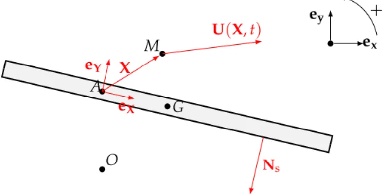
• Chapter1introduces in details the typical section model used in this the-sis. The dimensional and non-dimensional parameters are defined as well as the governing equations. Two variants of the Arbitrary Lagrangian Eulerian formalism, used to handle the moving fluid domain, are intro-duced. The technical details on the finite element spatial discretization of the Navier–Stokes equations are provided. Finally, a classical time-marching approach for integrating the fluid-structure equations is pre-sented, as it will serve as a reference across the manuscript. This chapter is mostly meant to offload the rest of the manuscript from the cumber-some technical details inherent to fluid-structure interaction.

• In chapter 2, we present in extensive details the weakly nonlinear ap-proach for the typical aeroelastic section. We also introduce a Hessian-based mesh adaptation framework that is used in the subsequent sections to efficiently explore the parameter space. The chapter ends with a val-idation of the weakly nonlinear results against reference fully nonlinear time-marching solutions.

• Chapter3is dedicated to the Time Spectral Method. As a (long) preamble, TSM is replaced in the more global zoology of harmonic balance meth-ods. A classification borrowed from spectral methods in space is used to organize the discussion. The core of the chapter presents the Newton— Krylov solution method and introduces the so-called block-circulant pre-conditioner that is at the core of the efficiency of the method when large number of harmonics are used. A parallelization in time is also presented. Several numerical experiments are reported to assess the robustness of the preconditioner. The method is applied first on cases where the solution frequency is known (forced oscillations) and then extended to the case of unknown frequency (self-sustained oscillations).

(28)

13

2. The second part of the thesis is dedicated to the physical analysis of the bi-furcation associated to the coupled-mode flutter instability of the aeroelastic section in laminar flows:

• We start our explorations in chapter 4 by revisiting the linear stability analysis of the typical section in low-Reynolds number flows. In addi-tion to coupled-mode flutter, divergence and vortex-induced vibraaddi-tions are also obtained. The thresholds for these different instabilities are com-puted while varying the solid-to-fluid mass ratio, thus allowing to build neutral curves for each type of instability. The effect of the Reynolds number is explored and comparisons are proposed with classical low-dimensional flow models such as quasi-steady models or the Theodorsen model.

• Chapter5focuses on exploring the effects of low-Reynolds number fluid nonlinearities on the type of flutter bifurcation (subcritical or supercrit-ical). The weakly nonlinear analysis is first used to explore parametri-cally the type of bifurcation for different solid-to-fluid mass ratios and Reynolds numbers. A decomposition of the cubic coefficient of the nor-mal form of the flutter bifurcation is introduced so as to identify the con-tributions of the different nonlinearities and spatial locations with respect to the type of the bifurcation. Then, the highly nonlinear regime is ex-plored by using results from both the Time-Spectral Method and refer-ence time-marching solutions. For certain parameters, a unusual bifur-cation scenario is obtained and is discussed with respect to unexplained experimental results in the literature.

• We conclude our exploration of the flutter bifurcation in chapter6by in-vestigating the solutions obtained up to 15% above the critical velocity, in a supercritical case. The bifurcation is first explored with reference time-marching solutions. Then a Floquet stability analysis is performed in order to explain the time-marching results. To that end, an original method based on the analysis of the spectrum of the linearized TSM op-erator is presented. The results from the Floquet analysis are analyzed and compared to the time-marching solutions, allowing to highlight the mechanism responsible for the observed time-marching results.

3. The third part of this thesis aims at initiating the extension of the solution methods used in the previous chapters for two-dimensional flows, to the three-dimensional case. It is composed of only one chapter.

• Chapter 7 focuses on performing large-scale purely hydrodynamic (the structure is fixed) linear stability analysis of incompressible flows. To this end, the methods used in the previous chapters for two-dimensional configurations are extended. The core issue of the linear solver for high-dimensional configurations is tackled by using a Krylov subspace method, preconditioned by the modified Augmented Lagrangian preconditioner. The performance of the preconditioner is first assessed on a two-dimensional test case and benchmarked with respect to other state-of-the-art alterna-tives. Then, a parallel implementation using the FreeFEM language and its PETSc/SLEPc interface is described and tested on a large-scale three-dimensional case.

(29)

14 Introduction

The results are finally summarized in the general conclusion, chapter8, leading to several propositions for future directions of research.