Development of two techniques for thermal characterization of materials : Scanning Thermal Microscopy (SThM) and 2ω method

HAL Id: tel-01207388

https://tel.archives-ouvertes.fr/tel-01207388

Submitted on 30 Sep 2015

HAL is a multi-disciplinary open access

archive for the deposit and dissemination of sci-entific research documents, whether they are pub-lished or not. The documents may come from teaching and research institutions in France or abroad, or from public or private research centers.

L’archive ouverte pluridisciplinaire HAL, est destinée au dépôt et à la diffusion de documents scientifiques de niveau recherche, publiés ou non, émanant des établissements d’enseignement et de recherche français ou étrangers, des laboratoires publics ou privés.

characterization of materials : Scanning Thermal

Microscopy (SThM) and 2ω method

Ali Assy

To cite this version:

Ali Assy. Development of two techniques for thermal characterization of materials : Scanning Thermal Microscopy (SThM) and 2ω method. Materials. INSA de Lyon, 2015. English. �NNT : 2015ISAL0001�. �tel-01207388�

Thèse

Development of two techniques for thermal

characterization of materials: Scanning

Thermal Microscopy (SThM) and 2

ω method

Présentée devant

L’Institut National des Sciences Appliquées de Lyon

Pour obtenir

Le grade de docteur

Formation doctorale : Énergétique

École doctorale : Mécanique, Énergétique, Génie Civil, Acoustique

Par

Ali ASSY

Soutenue le 03 Février 2015 devant la Commission d’examen

Jury MM.

O. BOURGEOIS Directeur de recherche CNRS (Institut Néel Grenoble) S. GOMES Chargée de recherche CNRS (CETHIL Lyon)

Rapporteur O. KOLOSOV Researcher - Reader (Lancaster University) S. LEFEVRE Maître de Conférences (INSA de Lyon) N. TRANNOY Professeur (Université de Reims)

R. VAILLON Directeur de recherche CNRS (CETHIL Lyon) Président S. VOLZ Directeur de recherche CNRS (Ecole Centrale Paris) Rapporteur J. WEAVER Professeur (Glasgow University)

SIGLE ECOLE DOCTORALE NOM ET COORDONNEES DU RESPONSABLE

CHIMIE CHIMIE DE LYON http://www.edchimie-lyon.fr

Insa : R. GOURDON

M. Jean Marc LANCELIN

Université de Lyon – Collège Doctoral Bât ESCPE

43 bd du 11 novembre 1918 69622 VILLEURBANNE Cedex Tél : 04.72.43 13 95

[email protected]

E.E.A. ELECTRONIQUE, ELECTROTECHNIQUE, AUTOMATIQUE http://edeea.ec-lyon.fr

Secrétariat : M.C. HAVGOUDOUKIAN [email protected]

M. Gérard SCORLETTI

Ecole Centrale de Lyon 36 avenue Guy de Collongue 69134 ECULLY

Tél : 04.72.18 65 55 Fax : 04 78 43 37 17 [email protected]

E2M2 EVOLUTION, ECOSYSTEME, MICROBIOLOGIE, MODELISATION http://e2m2.universite-lyon.fr Insa : H. CHARLES

Mme Gudrun BORNETTE

CNRS UMR 5023 LEHNA

Université Claude Bernard Lyon 1 Bât Forel

43 bd du 11 novembre 1918 69622 VILLEURBANNE Cédex Tél : 06.07.53.89.13

e2m2@ univ-lyon1.fr

EDISS INTERDISCIPLINAIRE SCIENCES-SANTE http://www.ediss-lyon.fr Sec : Samia VUILLERMOZ Insa : M. LAGARDE

M. Didier REVEL

Hôpital Louis Pradel Bâtiment Central 28 Avenue Doyen Lépine 69677 BRON

Tél : 04.72.68.49.09 Fax :04 72 68 49 16 [email protected]

INFOMATHS INFORMATIQUE ET MATHEMATIQUES http://infomaths.univ-lyon1.fr

Sec :Renée EL MELHEM

Mme Sylvie CALABRETTO

Université Claude Bernard Lyon 1 INFOMATHS Bâtiment Braconnier 43 bd du 11 novembre 1918 69622 VILLEURBANNE Cedex Tél : 04.72. 44.82.94 Fax 04 72 43 16 87 [email protected] Matériaux MATERIAUX DE LYON http://ed34.universite-lyon.fr Secrétariat : M. LABOUNE PM : 71.70 –Fax : 87.12 Bat. Saint Exupéry [email protected]

M. Jean-Yves BUFFIERE

INSA de Lyon MATEIS

Bâtiment Saint Exupéry 7 avenue Jean Capelle 69621 VILLEURBANNE Cedex

Tél : 04.72.43 83 18 Fax 04 72 43 85 28 [email protected]

MEGA MECANIQUE, ENERGETIQUE, GENIE CIVIL, ACOUSTIQUE http://mega.ec-lyon.fr

Secrétariat : M. LABOUNE PM : 71.70 –Fax : 87.12 Bat. Saint Exupéry [email protected]

M. Philippe BOISSE

INSA de Lyon Laboratoire LAMCOS Bâtiment Jacquard 25 bis avenue Jean Capelle 69621 VILLEURBANNE Cedex

Tél :04.72 .43.71.70 Fax : 04 72 43 72 37 [email protected]

ScSo ScSo* http://recherche.univ-lyon2.fr/scso/ Sec : Viviane POLSINELLI

Brigitte DUBOIS Insa : J.Y. TOUSSAINT

M. OBADIA Lionel Université Lyon 2 86 rue Pasteur 69365 LYON Cedex 07 Tél : 04.78.77.23.86 Fax : 04.37.28.04.48 [email protected]

To the memory of

Hassan Khalil (Grandpa) and Ali Jamil Khalil

This thesis is the result of many experiences I encountered during the period of my work at the CETHIL laboratory. I wish to acknowledge many remarkable individuals who helped me achieve the works that are presented in this manuscript.

First, I would like to thank all the members of the jury for their participation in the defense and for their comments. I thank the reviewers Oleg Kolosov and Jonathan Weaver for their careful reading of the manuscript and their reports on the whole study. I thank Sebastian Volz, the president of the jury, for useful discussions. I also thank Nathalie Trannoy and Olivier Bourgeois for their efforts during the examination of the manuscript. I enjoyed meeting all of you either during past conferences or during the defense and I hope our paths will cross in the near future.

I would like to express my gratitude to my PhD supervisors, Séverine Gomès and Stéphane Lefèvre.

Séverine, you already proved that you’re an excellent researcher and a great advisor. I will be always grateful for the opportunities and the freedom you gave me during the work.

During my PhD journey, I was a member of the MINT group (Micro and Nano Scale Heat Transfer group). The meetings and the discussions I had with the different group members gave me the opportunity to enhance my knowledge in the different current studies in our domain. Many thanks go to Rodolphe (Vaillon), the coordinator of this group, for his great sense of organization and management. I’m obliged here to thank Olivier C (Chapuis) for long and fruitful scientific discussions and for making me more curious and motivated. I also thank Olivier M (Merchiers) whom I consider a friend in our lab. I have to thank the other members of our group for the great moments we had during the meetings (Trang, Wassim, Farida (“je prends ce que je veux!!”), Ahmad, Mouhannad, Sylvie, Etienne, David, Olivier D, Carolina, Elyes, Yanqing (Ivy)….). Special thanks go to Trang for being funny all time (ah bon!) and to Wassim for his beautiful loud laugh. The atmosphere in the group was always warm and lovely.

I would like to thank some people, with whom I collaborate, for their warm welcome: Antoine and Pascal from ILM Lyon, Annie and Pierre from CLYM Lyon, and Nicolas Horny from GRESPI Reims.

I appreciate the great moments I had with different persons in the lab. Thanks to Jocelyn Bonjour, the director of the lab, for his understanding and listening ear. Thanks to Florence,

mention Corinne D, Sophie, and Christine D. I also thank the technical staff in our lab (even though they don’t care about those ‘nanoscale stuff’): Nico (et ses 7 laux et son équipe de Grenoble), Joël (le grand), Christophe Ducat (malgré que tu es Stéphanois), Bernard, Loïc, Bertrand… I won’t forget the special moments I had with the actual and former PhD students and postdoctoral researchers. For these moments, I thank Léon (and his English classy gestures), Aurélia (et son dragon ball!!), Auline, Lucie, Sébastian, Mathieu Labat, Pablo, Kim (oppa gangnam style !!), Zakaria Slimani, Damien (et son esprit de syndicats), Yun-Xin, Anna, Wei, Kévin (ses doodles qui se convergent jamais!!), Christophe Daverat, Pierrick (et son esprit 50 % corse – 50 % breton), Céline, Thibault B, Marcella, Christophe Kinkelin (toujours le dernier pour finir un repas!!), Daha (“muscles toi Daha”)…

I would like to thank my former officemates, Roula (“oufffffff”- and her great meals) and Matthieu Zinet (“heuresement il y a la voiture de Matthieu!!”)… Infinite thanks to both of them for being such good friends all time. I would like to wish the best for the new ones Sandra (Allez Auxerre!! – Kapo et Cissé allez allez) and Chi-Kien (et son robot!!).

I was lucky outside the lab to meet and to be surrounded by great people who became close friends. Many thanks go to those Lebanese friends who made the ambiance funny and joyful. Thanks to Srour (and his superb meals - open a restaurant man!!), Mortada (long football matches), Sabbah (and his African style meals - Come On You Gunners COYG!!), Mozannar (and his technology equipments), Mouazzen (and his endless guarantees), Zeinab (stop being always late girl!! Fortunately, you’re funny to compensate that), Banjak (stop lifting weights man!! You’re already a beast!!), Ankouni (and his delicious burgers), Tarhini (and his “lost village”!!), Inas and Nour, Hodroge, Hammoud, Khashman, Fardoun (and his hoummous), Damergi…

Big thanks to Romain and Tere, who were amazing during all of this period… Romain, you made me fall in love with Olympique Lyonnais (Allez OL!) and with rugby. Superb you’re man!! Tere, muchas gracias señorita for being supportive all the time. Many thanks go to for Tristan (with his French charm – ‘ton nom est déjà Amoureux, qu’est-ce qu’on peut ajouter ?!’) and Ainhoa (ijo polaco!!). I also thank the couple Sylvain (and his political analysis) and Pepa (you eat a lot girl really!!) for the beautiful moments we had in Lyon.

Special, huge, and unique thanks go to the special Esti (Estitxu) for her endless support and her beautiful spirit. Hat tip. Eskerrik asko. Que bonito Candanchu Con O Sin Nieveeeeee!!

later to follow my ambitions. Hopefully, one day I will be able to give them back just a little from what they gave me all time. I also thank my cute siblings, my sister Fatima (Fattouma – and her fiancé too ‘oh!’) and my brother Hussein (Nayno) for being the greatest people I can have. Many thanks also go to my big family including Grandparents, Cousins, Aunts and Uncles (lots of love to you…).

Two techniques to characterize the thermal properties of materials and to analyze the heat transfer at the micro/nanoscales have been studied and are presented in this manuscript. The first technique is the Scanning Thermal Microscopy (SThM), an Atomic Force Microscopy (AFM)-based technique. Operating in its active mode, the AFM probe integrates a resistive element that is electrically heated. Used in AFM contact mode, it allows the localized thermal excitation of the material to be studied. The determination of the sample thermal properties requires the analysis of the probe thermal response through the modeling of the probe-sample system including its surrounding. With the help of a review of SThM studies, the current scientific questions and the analytical models used to analyze the probe-sample system are explored. Special attention is given tothe probe-sample thermal interaction thatconditions the tip-sample interface temperature. Reducing the probe size requires a more in depth study of the physics of the heat transfer mechanisms of this interaction. In this work, a new methodology for studying and specifying the heat rate exchanged between a probe and a sample through thermal conduction through water meniscus has been established. The methodology is based on the analysis of the dependence of force-distance curves on probe temperature obtained in ambient air. It was applied with samples of different thermal properties, surface roughness and wettability to three resistive probes different in size and heater configurations: Wollaston, KNT and doped silicon (DS) probes. Whatever the probe and the sample are, the contribution of water meniscus in the probe-sample interaction has been shown to be lower than the one of air. Moreover, for the Wollaston and KNT probes, the parameters of a model based on a description of the probe-sample system using a network of thermal resistances are identified from measurements performed under ambient and vacuum conditions. The thermal conductances at the solid-solid contact were determined for various samples. This allowed identifying the phonon transmission coefficient in the case of KNT probe and a nonmetallic sample. Experimental results and numerical simulations for measurements performed under ambient conditions have demonstrated that the thermal interaction parameters of the heat conduction through air strongly depend on the sample thermal conductivity. Improvements of the current calibration methodology for thermal conductivity measurement have been proposed. The variation of sample roughness during the calibration and measurements may be an issue. Moreover, the sensitivity to sample thermal conductivity for the Wollaston and KNT probes is shown to be strongly reduced for thermal conductivities larger than 10 and a few W.m-1.K-1 respectively.

The second technique developed in this thesis is a less local thermal analysis method. It operates by contact, requiring the implementation of the sample surface with a network of resistive wire probes. One wire of the network is heated by an alternating current at frequency

f and has the role of heating source, continuous and at 2f frequency, for the sample. The other

wires are sensors of temperature (method "2ω"). A 2D analytical model, based on the principle of thermal-waves, was developed to identify the effective thermal properties of anisotropic samples from experimental measurements with the technique. This model can be reduced to a simplified 1D model in the case of diffusive, homogeneous and isotropic materials. Finite element simulations and this model were used to design the experimental set-up and validate the method with pure silicon. The results obtained at sample temperatures ranging from ambient to 500 K are consistent with literature.

Keywords: thermal techniques, Scanning Thermal Microscopy, micro and nanoscale heat transfer, thermal conductance, thermal conductivity, phonon transmission coefficient, microresistors, water meniscus

Deux techniques de caractérisation thermique des matériaux et d’analyse du transfert de chaleur aux micro- et nano- échelles ont été étudiées et sont présentées dans ce mémoire. La première technique est la microscopie thermique à sonde locale (SThM). La pointe d’un microscope à force atomique intègre un élément résistif. Utilisée en mode contact, cette pointe, chauffée par effet joule, permet l'excitation thermique localisée de l’échantillon. La détermination des propriétés thermiques de l’échantillon nécessite l'analyse de la réponse de cette pointe avec un modèle du système sonde-échantillon et de son environnement. Un état de l'art général des études réalisées en SThM permet de poser les questions scientifiques actuellement traitées dans le domaine ainsi que les modèles utilisés pour analyser le système pointe-échantillon. Une attention particulière est accordée à l'interaction thermique sonde-échantillon. Sa compréhension nécessite d’être approfondie. L’étude ici présentée tient compte des propriétés thermiques, de la rugosité et de la mouillabilité de la surface de différents échantillons. Une nouvelle méthodologie est établie pour la spécification du transfert de chaleur échangée par conduction thermique au travers du ménisque d’eau formé au contact sonde-échantillon. Cette méthodologie est basée sur l'analyse de la dépendance à la température de la sonde des courbes de force-distance obtenues à l'air ambiant. Elle est appliquée à trois sondes de taille, forme et constitution différentes: la sonde Wollaston, la sonde KNT et une sonde en silicium dopé. Quels que soient la sonde et l'échantillon, la contribution du ménisque d’eau à l'interaction est montrée être inférieure à celle de l'air. Par ailleurs, pour les sondes Wollaston et KNT, les paramètres d'une modélisation, basée sur une description du système sonde-échantillon avec un réseau de conductances thermiques, sont identifiés à partir de mesures effectuées à l’ambiante et sous vide. La conductance thermique au contact solide-solide est déterminée pour différents échantillons. Cela a permis d’identifier le coefficient de transmission de phonons dans le cas de la sonde KNT et d’échantillons non-métalliques. Nos résultats expérimentaux et de simulations numériques pour les mesures effectuées sous air démontrent que les paramètres utilisés pour décrire la conduction thermique via l’air dépendent fortement de la conductivité thermique de l'échantillon. Aussi des améliorations de la méthodologie actuelle d'étalonnage pour la mesure de la conductivité thermique sont proposées. Il est en outre montré que la variation de la rugosité de l'échantillon lors de l'étalonnage et de mesures doit être prise en compte. La sensibilité à la conductivité thermique pour les sondes Wollaston et KNT est part ailleurs montrée fortement réduite pour les matériaux de conductivité thermique supérieure à 10 et quelques W.m-1.K-1 respectivement.

La seconde technique développée est une méthode d’analyse thermique moins locale nécessitant l’instrumentation de la surface de l’échantillon avec un réseau de sondes résistives filiformes. L’un des fils du réseau, chauffé par un courant alternatif à la fréquence f, a le rôle de source excitatrice continue et à la fréquence 2f de l’échantillon. Les autres fils sont des capteurs de la température (méthode «2ω»). Un modèle analytique 2D, basé sur le principe des ondes thermiques et développé pour identifier les propriétés thermiques d’échantillons anisotropes est présenté. Ce modèle peut être réduit à un modèle simplifié 1D dans le cas de matériaux diffusifs, homogènes et isotropes. Des simulations par éléments finis et avec ce modèle ont été utilisées pour dimensionner le montage expérimental et valider la méthode sur un échantillon de silicium pur. Les résultats obtenus à des températures de l’échantillon variant de l’ambiante à 500 K corroborent ceux de la littérature.

Mots-clés: méthodes thermiques, microscopie thermique à sonde locale, transfert de chaleur aux micro- et nano-échelles, conductance thermique, conductivité thermique, coefficient de transmission des phonons, méthode à fils résistifs déposés, ménisque d’eau

Abbreviation AFM ESEM MD NEMD SEM SPM SNOM SThM Symbol Term

Atomic Force Microscope

Environmental Scanning Electron Microscope

Molecular Dynamics

Non-Equilibrium Molecular Dynamics

Scanning Electron Microscope

Scanning Probe Microscope

Scanning Near-Optical Microscope

Scanning Thermal Microscopy

Variable Unit

a Thickness of the meniscus m

A Accommodation factor

ac Radius of mechanical contact m

b Equivalent radius of the thermal exchange m

bw Wire width m

C Heat capacity J.Kg-1.K-1

Cp Heat capacity at constant pressure J.Kg-1.K-1

Cpa Heat capacity of acoustic phonons J.Kg-1.K-1

Cv Heat capacity at constant volume J.Kg-1.K-1

D Diameter m

d Thickness m

d0 Density kg.m-3

ds Tip-sample separation distance m

E Young modulus Pa

Fad Adhesion force N

Fcap Capillary forces N

Fpo Pull-off forces N

Gr Grashof number

Gair Thermal conductance through air W.K-1

Gatom-atom Thermal conductance of atom-atom contact W.K-1

Gc Contact thermal conductance W.K-1

Gep Volumetric phonon-electron coupling constant W.m-3.K-1

Geq Equivalent thermal conductance Geq=(GcGs)/(Gc+Gs) W.K-1

Gp Probe thermal conductance W.K-1

Gp-w Probe-water thermal conductance W.K-1

Gw-s Water-sample thermal conductance W.K-1

GQ Quantum thermal conductance W.K-1

Grad Thermal conductance of radiation W.K-1

Gs Thermal conductance of the sample W.K-1

Gss Thermal conductance of the solid-solid contact W.K-1

Gtotal, meniscus The total conductance of the water meniscus W.K-1

Gw Thermal conductance through the water meniscus W.K-1

h Heat transfer coefficient W.m-2.K-1

hg Global linearized convective and radiative losses W.m-2.K-1

hk Meniscus height m

I Electrical current A

K1 Correction factor

kx X-component of the wave vector

L Length m

N Number of phonon modes

Nu Nusselt number

p Fin perimeter m

P Pressure bar

Pa Probe Joule power - Probe free in air W

Pc Probe Joule power - Probe in contact with sample W

Pp Power dissipated in the probe W

Pd Power dissipated in the heater (heating wire) W

Prms Power per unit heater length W.m-1

Pr Prandtl number

Q Heat flux W

R Electrical resistance Ω

Ra Rayleigh number

Ra Tip apex radius m

Rar Arithmetic value of roughness m

Rb Thermal boundary resistance m2.K.W-1

Rbp Thermal boundary resistance of the phonon-phonon

coupling

m2.K.W-1

Rbe Thermal boundary resistance of the phonon-electron

coupling

m2.K.W-1

Rg Gas constant J.mol-1.K-1

Rs Spreading thermal resistance K.W-1

Rth Interface thermal resistance K.W-1

Rp-p Peak-to-peak roughness m

Rsph Sphere radius m

Rtip Tip thermal resistance K.W-1

RH Relative humidity

r1 Smallest meniscus radius m

r12 Reflection coefficient at the tip-sample interface

r2 Largest meniscus radius m

S Section m2

rk Cavity radius m

T Temperature K

Ta Ambient Temperature K

Tm Probe mean temperature °C

t1 Film thickness m

t12 Phonon transmission coefficient

V Voltage V

Vair Velocity of air molecules

VDC Continuous voltage V

Vm Molar volume m3.mol-1

V_3ω Third harmonic voltage V

w Width m

wd Dupré Energy of adhesion N

ws Sample width m

Greek letters

α Thermal diffusivity m2.s-1

β Temperature coefficient of the electrical resistivity K-1

γw Water surface tension N.m-1

ε Surface emissivity

θ Relative temperature K

θ Mean Relative temperature K

θDC Continuous relative temperature K

θ2w Second harmonic relative temperature K

γ Cp/Cv

λmax Maximum wavelength of thermal radiation µm

λ Thermal conductivity W.m-1.K-1

λpp Phonon-phonon thermal conductivity W.m-1.K-1

λw Thermal conductivity of water W.m-1.K-1

λmax Maximum wavelength of thermal radiation m

Λ Phonon mean free path m

µ Diffusion length m

ν Poisson ratio

νpa Velocity of acoustic phonons m.s-1

ρ Electrical resistivity Ω.m-1

χ Wave vector along z

Ф Phase lag °

Фd Heat flow density W.m-2

Фref Ratio of heat power

ω Angular frequency Rad.s-1

ACKNOWLEDGEMENTS ... 5 ABSTRACT ... 9 NOMENCLATURE ... 12 TABLE OF CONTENTS ... 18 LIST OF FIGURES ... 21 LIST OF TABLES ... 26 GENERAL INTRODUCTION ... 27

CHAPTER 1: SCANNING THERMAL MICROSCOPY (STHM): STATE OF THE ART AND EXPOSITION OF THE ISSUES ... 31

1.1 Scanning Thermal Microscopy (SThM) ... 32

1.2 Operational modes of resistive SThM probes ... 32

1.3 Resistive probes description ... 33

1.3.1 The Wollaston wire probe ... 33

1.3.2 The KNT probe (the palladium or GLA probe) ... 34

1.3.3 Silicon nanoprobes ... 35

1.4 Approaches of the measurement ... 36

1.4.1 The Wollaston probe ... 36

1.4.2 The palladium probe ... 41

1.4.3 Silicon nanoprobes ... 42

1.5 Heat losses through the air ... 45

1.6 Thermal spreading resistance ... 46

1.7 Heat transfer mechanisms between SThM probes and sample ... 47

1.7.1 Heat transfer through radiation ... 48

1.7.2 Heat transfer at solid-solid contact ... 50

1.7.3 Heat transfer though water meniscus ... 55

1.7.4 Heat transfer through air ... 59

1.8 Conclusions ... 65

CHAPTER 2: ANALYSIS OF HEAT TRANSFER IN THE WATER MENISCUS AT THE TIP-SAMPLE CONTACT IN STHM ... 68

surface 71

2.1.3 Young-Laplace and Kelvin Equations ... 72

2.2 Methodology developed and used to investigate the temperature-dependence of the meniscus ... 73

2.2.1 Experimental approach ... 73

2.2.2 Derived parameters: Meniscus parameters and thermal conductance of probe-sample heat transfer through water ... 77

2.2.3 Results ... 80

2.2.4 Effect of roughness on the pull-off forces on hydrophilic surfaces ... 82

2.2.5 Measurement of the pull-off forces on hydrophobic surface ... 84

2.3 Preliminary experiments performed in the frame of the development of a SThM-ESEM combined system ... 86

2.4 Conclusion ... 89

CHAPTER 3: PROBE-SAMPLE THERMAL SYSTEM IN DC SCANNING THERMAL MICROSCOPY INVESTIGATED WITH THE WOLLASTON PROBE . 92 3.1 Influence of the probe temperature Tm on the thermal signal ΔP/Pc and on Gp ... 93

3.2 Influence of the probe mean temperature Tm on Gp ... 94

3.3 Thermal conductance at the solid-solid contact Gss ... 96

3.4 Measurements under ambient conditions ... 101

3.4.1 Determination of the coefficient h of the heat losses to the environment ... 101

3.4.2 Heat conduction through air to the sample ... 102

3.4.3 Effect of roughness of the samples on the heat transfer to the sample ... 111

3.5 Variations of ΔP/Pc as a function of Tm ... 113

3.6 Approach for a more accurate thermal conductivity calibration ... 114

3.7 Determination of the thermal conductivity of Ba8Si46 clathrates ... 115

3.8 Conclusion ... 116

CHAPTER 4: DC SCANNING THERMAL MICROSCOPY WITH PROBES OF NANOSCALE RADIUS OF CURVATURE ... 119

4.1 Study of the probe-sample thermal with the KNT probe ... 120

4.1.1 Thermal conduction through the water meniscus... 120

4.1.2 Thermal conduction through the solid-solid contact: ... 125

4.1.3 Thermal conduction through air ... 128

4.2 Study of the probe-sample thermal system with doped silicon (DS) probes: ... 130

4.4 Conclusion ... 136

CHAPTER 5: DEVELOPMENT OF A TECHNIQUE FOR INVESTIGATION OF THERMAL PROPERTIES OF SOLID MATERIALS AT TEMPERATURES ABOVE THE AMBIENT ... 139

5.1 Main thermal techniques using deposited resistive heater and probe ... 140

5.2 Proposed method ... 146

5.2.1 General principle ... 146

5.2.2 Associated thermal modeling in the alternating regime ... 147

5.3 Establishment of the method for a simple reference material ... 151

5.3.1 Thereference material ... 151

5.3.2 Design of the resistive wire array ... 151

5.4 Analysis of the influence parameters ... 157

5.4.1 Effect of the heat losses on TDC and ΔT2ω ... 157

5.4.2 Effect of the resistance of contact between the heater and the wire... 158

5.5 Way for the simplification of the thermal model: 1D approach ... 159

5.6 Experimental Set-up ... 161

5.7 Experimental results ... 162

5.8 Case of anisotropic samples ... 164

5.8.1 In plane thermal conductivity ... 164

5.8.2 Cross-plane thermal properties ... 168

5.9 Conclusions and Perspectives ... 169

GENERAL CONCLUSIONS ... 172

APPENDIX A: NTEGRA PROBE NANOLABORATORY, THERMAL CONTROL UNIT AND THE NANOTA2 ... 176

List of Figures

Figure 1.1. Description of the principle of the technique ... 32 Figure 1.2. a) Description of the Wollaston probe b) SEM (Scanning Electron Microscope) image of the Wollaston probe. ... 34 Figure 1.3. Description of the KNT probe (courtesy of Kelvin NanoTechnology). ... 34 Figure 1.4. SEM images of the palladium probe. ... 35 Figure 1.5. SEM images of the Anasys Instruments probes (Anasys instruments). ... 35 Figure 1.6. Schematic of the description of the Wollaston probe [22]. ... 37 Figure 1.7. The heat balance on a element dx of the Pt90/Rd10 wire [22]. ... 38 Figure 1.8. Description of the network of the thermal conductances of the probe-sample system. ... 39 Figure 1.9. The description of the KNT probe [28]. ... 42 Figure 1.10. Modeling the tip-sample system as given by Gotsmann et al. [12]. ... 44 Figure 1.11. Modeling the scattering at the interface through the phonon reflection coefficient

r12 [12]. ... 44

Figure 1.12. Heat flow lines and isotherms during the conduction from a localized heat source [43]. ... 47 Figure 1.13. Schematic of the different heat mechanism that operate between the probe and the sample [13]. ... 48 Figure 1.14. Variation the heater temperature of a silicon probe during the approach and retract curves [45] (Frequency of 1 Hz – P = 10-5 mbar). ... 49 Figure 1.15. The variation of the deflection and V_3ω probe voltage as a function of the

probe/sample distance. The probe used here is the palladium probe and the sample is made of Silicon (P=10-5 mbar and Iprobe= 308 µA [28]). ... 52

Figure 1.16. Variation of the thermal signal ΔP/Pc as a function of the probe/sample distance

between a Wollaston wire probe and a monocrystalline silicon sample at different levels of pressure[57]. ... 53 Figure 1.17. Variation of the equivalent conductance Geq as a function of the force signal ΔI

for measurements performed on a sample of Hafnium under ambient conditions [22]. ... 54 Figure 1.18. Approach and retraction curves between a flat-punch tip and taC sample a) Variation of the heater temperature b) Evaluation of the thermal resistance at the tip-sample contact (P ≃ 6 × 10-6 mbar) [58]. ... 55 Figure 1.19. Schematic of the meniscus when the probe is in contact with the sample. ... 56 Figure 1.20. A model of the thermal resistances between the substrate and the tip in the

experiment of Luo [59]. ... 57 Figure 1.21. Variation of the ratio Gprobe/Gcontact as a function of the heater temperature Theater

in the experiment of Thiery et al. [61]. ... 58 Figure 1.22. Variation of the equivalent resistance Req=1/Geq as a function of the distance

between the Wollaston probe and a Silver sample [22]. ... 60 Figure 1.23. Differential tension (V) as a function of the separation distance between the probe and the sample. The red line and the green line represent respectively the diffusive model and the complete regime [27]. ... 61 Figure 1.24. Variation of the probe 3ω voltage V3ω as a function of the pressure when the probe in contact and out of contact with a Yttrium oxide sample [27]. ... 62 Figure 1.25. (a) Differential tension as a function of the probe/sample distance for a sample of Niobium (λ= 59 W.m-1.K-1). A zoom at the contact zone is shown in Figure (b) [27]. ... 63 Figure 1.26. Sensitivity of the palladium probe for materials of various thermal conductivities of samples [16]. ... 64

Figure 1.27. Variation of the probe electrical resistance when the tip contacts the sample as a function of the sample thermal conductivities. The simulations accounts for three

conductivities of the probe materials [66]. ... 65 Figure 2.1. Schematic of the principle of Dip-pen nanolithography (DPN) [76]. ... 70 Figure 2.2. Evolution of the water film thickness as a function of the relative humidity for three types of materials: chromium Cr, copper Cu and gold Au. The measurement were

performed using a scanning Kelvin probe force microscope (SKPFM) [87]. ... 72 Figure 2.3. Schematic of a capillary confined in a longitudinal tube [95]. ... 72 Figure 2.4. Image of the contact between the water droplet and the sample of Ge. ... 74 Figure 2.5. Spectroscopy curves performed on Germanium (Ge) for different probe mean temperature: (a) Ambient temperature, (b) Tm= 130 °C and (c) Tm= 230 °C. ... 75

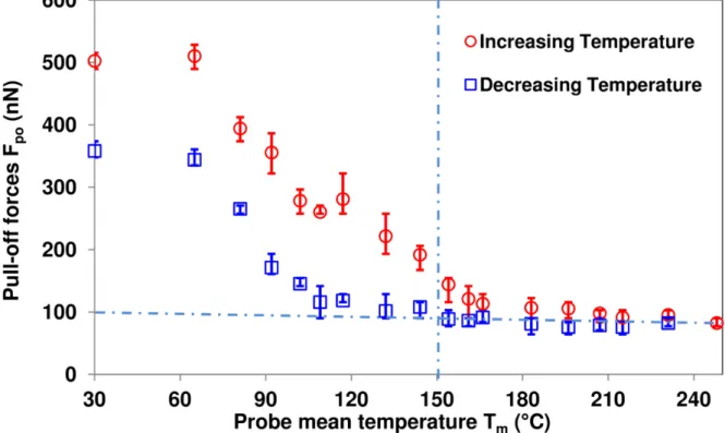
Figure 2.6. Dependence of the meniscus pull-off force on the tip−sample contact time [100]. ... 76 Figure 2.7. Variation of the pull-off forces Fpo as a function of the probe mean temperature Tm

for the sample of polished germanium. ... 77 Figure 2.8. Schematic of the meniscus when the probe is in contact with the sample. ... 78 Figure 2.9. Scanning Electron Microscopy SEM image of a Wollaston wire probe apex. ... 79 Figure 2.10. Schematic of a sphere and a cylinder with their radii of curvature ... 79 Figure 2.11. Radius of the curvature of the meniscus r2 as a function of the Wollaston probe

mean temperature Tm for the Ge sample (Ta= 30 ⁰C, RH= 40 %). ... 80

Figure 2.12. Total thermal conductance of the meniscus Gtotal, meniscus as a function of the

Wollaston probe mean temperature Tm for the Ge sample (Ta= 30 ⁰C, RH= 40 %). ... 81

Figure 2.13. Variation of the pull-off forces Fpo as a function of the probe mean temperature

Tm for the sample of rough germanium. ... 83

Figure 2.14. Schematic illustration of the meniscus of a contact between the probe and a surface asperity [94]. ... 84 Figure 2.15. Variation of the pull-off forces Fpo as a function of the probe mean temperature

Tm for the sample of graphite. ... 84

Figure 2.16. Pull-off force as a function of RH measured between a hydrophobic tip and a flat silicon sample [110]. ... 85 Figure 2.17. ESEM image of the water meniscus formed at the contact between Wollaston wire and germanium sample (Tsubstrate≃ 2 °C, RH ≃ 90 %). ... 86

Figure 2.18. Meniscus height (nm) as a function of the relative humidity for a SiN cantilever tip in contact with a silicon substrate at a temperature of 5 °C . ... 88 Figure 2.19. ESEM image of a liquid film on a Ge substrate showing two different zones of the liquid film (Tsubstrate≃ 2 °C, RH between 95 and 100 %). ... 88

Figure 2.20. Schematic diagram of the cases (a) where the electron beam is not focused (b) and when it is focused in an ESEM chamber on the probe-sample contact. ... 89 Figure 3.1. Variations of the probe Joule power relative difference as a function of the probe mean temperature when the probe contacts a sample of germanium Ge (Ta = 30 °C and RH=

40 %). ... 93 Figure 3.2. Variations of the probe conductance Gp as a function of the probe mean

temperature Tm. ... 95

Figure 3.3. Variation of λPt/Rd as a function of Tm as determined by Raphael [42]. ... 96

Figure 3.4. ΔP/Pc Calibration curves obtained by David [56] under ambient conditions (ac =

7.5 nm, Gair =4.5 × 10-6 W.K-1). ... 97

Figure 3.5. Variation of the thermal signal for the three materials (MICA, Ge and Si) under vacuum conditions (Tm= 140°C, RH=40 %, Ta=30 °C). ... 100

Figure 3.6. Estimation of the thermal conductance at the solid-solid contact Gss for the three

materials (MICA, Ge and Si). ... 100 Figure 3.7. Thermal boundary resistance Rb (m2.K.W-1) identified for the three materials

(MICA, Ge and Si). ... 100 Figure 3.8. Schematic of the probe in two different positions. ... 102 Figure 3.9. Voltage of the probe in different conditions for different tilts of the probe. ... 102 Figure 3.10. ΔP/Pc variation as a function of the thermal conductivity λs (Ta=30°C, RH=40%).

... 105 Figure 3.11. Schematic of the heat flux lines for two samples of different thermal conductivity

λs. ... 105

Figure 3.12. Variation of bair and Gair as a function of λs and their corresponding fitting

curves (a1= 1.05E-04, b1=-2.32, c1=3.42E-06, d1=-0.04492; a2=7.77E-06, b2=-5.18E-04 , c2

=-5.47E-06, d2=-1.197). ... 106

Figure 3.13. The model of the probe being at proximity of the sample. ... 108 Figure 3.14. Calculated relative heat power transferred to the sample as a function of its thermal conductivity λs. ... 109

Figure 3.15. Variation of the temperature on the sample surface in the direction of the major axis X. ... 110 Figure 3.16. Variation of the temperature on the sample surface in the direction of the minor axis Y. ... 110 Figure 3.17. Variation of the thermal interaction radii bx, by and b’air as a function of the

thermal conductivity λs. ... 111

Figure 3.18. Variation of the thermal signal ΔP/Pc for the different samples of different

roughness parameters (Ta= 25 ⁰C, RH= 40 %). ... 113

Figure 3.19. Variation of the modeled ΔP/Pc as function of the probe mean temperature Tm for

the sample of germanium Ge. ... 114 Figure 4.1. Variation of the pull-off forces as a function of the probe mean temperature for the contact between KNT probe and samples of PI (red circles) and Ge (blue squares). ... 122 Figure 4.2. Network of thermal resistance in series as a description of the probe-sample thermal system. ... 122 Figure 4.3. Schematic description of the variation of Rsample and Δ as a function of λs. ... 123

Figure 4.4. Variation of the larger radius r2 of the meniscus as function of the probe mean

temperature Tm for the contact between KNT probe and samples of PI (red circles) and Ge

(blue squares). ... 124 Figure 4.5. Variation of the total thermal conductance of water meniscus Gtotal, meniscus as

function of the probe mean temperature Tm for the contact between KNT probe and samples

of PI (red circles) and Ge (blue squares). ... 125 Figure 4.6. Thermal conductance of the probe as a function of the probe mean temperature Tm

(P=0.28 mbar, Ta=30 °C). ... 127

Figure 4.7. Thermal signal ΔP/Pc for the two samples of Ge and Si (P = 0.28 mbar, Ta = 30

°C). ... 127 Figure 4.8. Thermal signal ΔP/Pc as function of the sample thermal conductivity λs (Ta=30 °C,

RH= 40 %). ... 128

Figure 4.9. Thermal signal ΔP/Pc as function of the sample thermal conductivity λs for Tm= 40

°C (blue circles) and Tm= 65 °C (red circles) (Ta=30 °C, RH= 40 %). ... 129

Figure 4.10. Monitoring the probe cantilever deflection as a function of the probe heating voltage of the three reference polymers. ... 131 Figure 4.11. Heating Voltage (V) as a function of the apex temperature Tap (°C). ... 131

Figure 4.12. Pull-off forces Fpo as a function of the apex temperature Tap for a contact

Figure 4.13. Pull-off forces Fpo as a function of the heater temperature for a contact between

the DS probe (AN-300) and silicon dioxide SiO2 sample [113]. ... 133

Figure 4.14. Variation of the larger radius r2 of the meniscus as function of the apex

temperature Tapfor the contact between DS probe and sample of Po (Ta=30 °C, RH= 40 %).

... 133 Figure 4.15. Variation of the total thermal conductance of water meniscus Gtotal, meniscus as

function of the apex temperature Tap for the contact between DS probe and sample of Po

(Ta=30 °C, RH= 40 %). ... 134

Figure 5.1. Schematic of 3ω method where a metallic wire (heating wire) is deposited on the sample to be characterized. ... 140 Figure 5.2. Schematic of the phase-shift method used by Zhang and Grigoropoulos [136]. . 144 Figure 5.3. The configuration of the sample used by Jang et al. [144]. ... 145 Figure 5.4. Schematic of method principle. ... 147 Figure 5.5. Top view of the model showing the distribution colored with isotherms while generating current amplitude Iac of 60 mA... 152

Figure 5.6. Variation of ΔT2ω for different lengths as a function of the distance from the heating wire. ... 153 Figure 5.7. Schematic of the implemented sample. ... 154 Figure 5.8. Process flow for the deposition of the metallic wires array. (a) Photolithography, (b) Metal deposition, (c) Lift-off process. ... 154 Figure 5.9. AFM 2D image of a gold wire. ... 155 Figure 5.10. The mask design showing the probe wires (in yellow) and the heater (in red). 155 Figure 5.11. Schematic of the 2D COMSOL model. ... 156 Figure 5.12. Variation of ΔT_2ω in the two COMSOL configurations (2D and 3D) as a function of the distance from the heating wire for Si sample (f= 40 Hz, ϵ=1, h= 5 W.m-2.K-1 and Iac=60

mA). ... 156 Figure 5.13. Effect of the heat losses on the temperature of the sample TDC in 2D and 3D

COMSOL configurations (Iac=60 mA). ... 157

Figure 5.14. Variations of ΔT2ω as a function of the distance from heating wire for different values of h and ϵ (Iac=40 mA, f=40 Hz). ... 158

Figure 5.15. Variation of ΔT2ω(K) (calculated in 2D COMSOL configuration) as a function of the distance of the heating wire (µm) for a perfect contact (Rth=0) and for Rth= 3 × 10-7

m2.K.W-1. ... 159 Figure 5.16. Comparison of ΔT_2ω between the analytical model, 2D numerical simulations and 1D approach (Iac=60 mA, ϵ=1 and h=5 W.m-2.K-1). ... 161

Figure 5.17. Comparison of the phase lag (º) between the analytical model, 2D numerical simulations and 1D approach (Iac=60 mA, ϵ=1 and h=5 W.m-2.K-1). ... 161

Figure 5.18. Schematic of the experimental set-up. ... 162 Figure 5.19. Electrical connections of the measurements. ... 163 Figure 5.20. Experimental variations ΔT_2ω as a function of the distance from the heating wire for Iac=60 mA and for different frequencies... 163

Figure 5.21. Experimental variations of the phase lag ϕ as a function of the distance from the heating wire for Iac=60 mA and for different frequencies. ... 163

Figure 5.22. Simulated Variation of the sample temperature TDC as a function of the distance

from the heating wire for the two cases: λx>> λz and λx<< λz (Iac=60 mA, ϵ=1, h=5 W.m-2.K-1).

... 165 Figure 5.23. Simulated Variation of ΔT_2ω as a function of the distance from the heating wire for the numerical simulations and the 2D analytical in the case of anisotropic sample (λx>> λz,

Figure 5.24. Simulated Variation of the phase lag ϕ as a function of the distance from the heating wire for the numerical simulations and the 2D analytical in the case of anisotropic sample (λx>> λz, Iac=60 mA, f=40 Hz and ϵ=1, h=5 W.m-2.K-1). ... 166

Figure 5.25. Simulated variation of the (a) phase lag (b) ΔT_2ω as a function of the distance from the heating wire for the numerical simulations and the analytical model in the case of anisotropic sample (λx<< λz, Iac=60 mA, f=40 Hz and ϵ=1, h=5 W.m-2.K-1). ... 167

Figure 5.26. Simulated variation of the (a) phase lag (b) ΔT_2ω as a function of the distance from the heating wire for the numerical simulations and the analytical model in the case of anisotropic sample (λx<< λz, Iac=60 mA, f=40 Hz and ϵ=1, h=5 W.m-2.K-1). ... 167

Figure 5.27. Variation of the phase lag ϕ as a function of the current frequency for the numerical simulations and the analytical model for the probing wire located at the back

surface of the sample (λx<< λz, Iac = 60 mA, f = 40 Hz and ϵ=1). ... 168

Figure 5.28. Variation of ΔT2ω as a function of the current frequency for the numerical simulations and the analytical model for the probing wire located at the back surface of the sample (λx<< λz, Iac=60 mA, f=40 Hz and ϵ=1). ... 169

List of tables

Table 1.1. Properties of the Wollaston wire probe. ... 33 Table 1.2. Dimensions of different silicon nanoprobes... 36 Table 3.1. ΔP/Pc results for the samples of Mica, Germanium and Silicon under vacuum

conditions (values of λs were given by the suppliers, Goodfellow and Neyco). ... 98

Table 3.2. List of the calibration samples used in the measurements with their roughness parameters measured with AFM (values of λs were given by the suppliers, Goodfellow and

Neyco). ... 103 Table 3.3. Identified parameters of the probe-sample thermal interaction for the two cases:

h=0 and h=3000 W.m-2.K-1. ... 104 Table 3.4. Mean values of Gair and bair for different intervals of the thermal conductivity λs.

... 106 Table 3.5. Samples with the values of their roughness parameters (Rar and Rp-p) and

corresponding identified thermal conductivity λs. ... 112

Table 4.1. Thermal interaction parameters Gair and bair determined for two different

temperatures. ... 129 Table 4.2. List of the reference polymers with their corresponding melting temperatures. (reference Anasys instruments). ... 131 Table 5.1. Thermal properties of pure silicon at different temperature levels. ... 151 Table 5.2. Measured properties of the wires. ... 155 Table 5.3. Si thermal properties experimentally determined. ... 164

General introduction

The understanding of heat transfer and the improvement of some industrial production processes require the development of sophisticated thermal metrologies. For micro and nanotechnologies in particular, these metrologies should be accurate in terms of measurement of the thermal parameters and spatial resolutions. A perfect example is thermal management in electronics [1]. It is indeed a crucial aspect for the design of integrated circuits due to the integration density achieved nowadays. Everything from the scale of the printed circuit board (a few cm) to that of elementary transistor (a few nm) must be designed to limit power consumption and to facilitate heat dissipation [2, 3]. All micro and nanosystems currently fabricated with microelectronics technology tools such as thin film based devices or micro and nanostructured components also raise similar issues. Moreover, these systems require a precise knowledge of the thermal properties of the constituting materials or of those considered for optimization. Another field is thermoelectric energy conversion, which is one of the ways that might help facing the energy challenge [4]. Searching for a larger thermoelectric figure of merit ZT is of paramount importance. One common feature of recently-discovered thermoelectric materials with ZT>1 is that most of them have very low lattice thermal conductivities [5]. The thermal properties of these new materials need to be characterized. More generally, the development of nanoscale metrologies is required to study of the effects of the nanostructuration process. This type of processes is used to confer revolutionary physical properties to materials. The understanding of the thermal impacts is the key that will allow the predictive modeling of the heat transfer in next-generation systems. It is essential for the design stage and for the improvement in terms of quality and security of systems.

From a fundamental point of view, there has been an urgent need to understand the physics of the heat transfer at the micro and nanoscales. In the case of heat transfer within nanostructures and nanostructured materials or of heat exchange between two systems, the macroscopic thermal models are not valid if the dimensions of the zones of thermal contact and systems become comparable to the mean free path of the heat carriers of the two systems. Several parameters can affect the heat transfer between two systems and they are not fully understood yet. They include the thermal properties of systems, the roughness of material surfaces, the wettability of surfaces, the temperature of materials, etc…

In terms of spatial resolution, the far field optical methods used to characterize the thermal properties of materials are limited by the diffraction limit [6]. In these techniques, the signal

detection is performed at distances larger than the wavelength. In order to achieve a better spatial resolution in the determination of thermal properties and studying the heat transfer at submicron scales, Scanning Thermal Microscopy SThM has been developed for more than 25 years [7, 8]. The major part of this manuscript is dedicated to the characterization of the measurement with this technique. Commercialized resistive probes of different spatial resolutions were used to study the thermal system composed by the probe interacting with the sample in SThM (called “probe-sample thermal system” in the manuscript). Such approach would provide a better understanding of the technique and seek its improvement. Another thermal technique, less local because requiring the deposit of resistive wire-probes on the sample surfaces was also developed. It is presented in the last part of the manuscript.

The first chapter introduces the SThM technique. It presents the three resistive probes used in this work. For each of these probes, a state of the art of researches is given in terms of the modeling of the probe-sample thermal system. The chapter presents the experimental and modeling investigations that studied the heat losses to the environment while working under ambient conditions. The heat transfer mechanisms of the heat transfer between the probe and the sample are presented: thermal radiation, thermal conduction at the solid-solid contact, thermal conduction through water meniscus formed at the probe-sample contact and through air. Based on literature researches, each heat transfer mechanism is detailed and analyzed in order to bring out the parameters that affect the mechanism. The tasks to deal with in this manuscript and the experimental conditions are defined.

The second chapter is dedicated to the study of the heat transfer through water meniscus with the Wollaston wire probe (a micrometric probe). Two potential applications related to the results of the study are first presented. The chapter gives then a new methodology to determine the characteristic dimensions of the meniscus, an effective dimensional parameter of the probe apex and the meniscus thermal conductance. The last section of this chapter discusses some preliminary results of experiments performed in an environmental scanning electron microscope (ESEM) in order to observe the water meniscus at the contact between a probe and a sample. This was motivated by the current development of a SThM-ESEM combined system at CETHIL.

Based on the comparison of experimental results obtained with results of simulation for various experimental conditions, a quantitative analysis of the conduction through the solid-solid contact and air is given in the third chapter for the Wollaston probe. The thermal conductance at the solid-solid contact is measured under vacuum conditions on polished

samples and the thermal boundary resistance at the tip-sample interface is determined. Later, the thermal conduction through air is determined while taking into account the sample thermal conductivity. The effect of roughness of different samples on the probe-sample thermal interaction is presented. Several criteria are proposed in order to improve the SThM calibration for thermal conductivity measurement.

Chapter 4 mainly focuses on measurement carried out with the KNT probe. Moreover, results obtained with the doped silicon DS probe are presented and discussed. Applying the methodology described in chapter 2 to these probes, the water meniscus conduction is studied on samples of different thermal conductivity. Besides, the results of measurements under vacuum conditions performed on different samples are presented for the KNT probe. The heat conduction at the tip-sample contact is investigated and the determination of the thermal boundary resistance for each sample is addressed. Using various reference samples and while working under ambient conditions, the sensitivity to the sample thermal conductivity is specified for the KNT probe. The last part of this chapter proposes an evaluation of the phonon transmission coefficient at the tip-sample contact.

The last chapter of the manuscript presents the concept of a technique to characterize the thermal properties of anisotropic samples. Based on contact thermal metrologies operating in AC regime, the technique allows studying samples at temperatures above the ambient. The technique is called the “2ω method”. Its principle and first results of experimental work and simulations for the technique validation are presented and discussed. The experimental results on a Si sample are compared with the literature studies. Later, numerical simulation works are presented in order to set a basis to identify the thermal properties of the sample in the in-plane and cross-plane direction of an anisotropic sample with the 2ω method.

1. Chapter 1: Scanning Thermal Microscopy

(SThM): State of the art and exposition of the

issues

Chapter 1

Scanning Thermal Microscopy (SThM): State of the

art and exposition of the issues

The Scanning Thermal Microscopy (SThM) with its better spatial resolution than the photothermal methods is used nowadays to characterize the thermophysical properties of materials. However the characterization of materials using SThM probes is still challenging and requires a better understanding and a proper modeling of the probe-sample system. Thus, any interpretation of the measurements must be accompanied with an appropriate modeling of the probe-sample system to identify precisely the properties of the considered materials. The investigation of the probe-sample system involves studying the heat transfers through three elements: 1) the probe 2) the sample and 3) their surrounding environment.

Therefore, this chapter summarizes, to present, a state of the art of the research studies that involves the SThM to characterize the sample thermal conductivity as well the heat transfer mechanisms between the probe and sample. It gives, in order:

- An introduction of the technique and the description of the resistive probes that are involved in this work.

- The thermal modeling of the probe-sample system currently proposed and used for the interpretation of SThM measurements obtained with these probes.

- The research works performed for studying, describing and identifying the heat losses from the probe to the environment medium.

- The heat mechanisms that exist between the probe and the sample depending on the conditions of experiments.

Based on this commented review, the scientific tasks to deal with in the upcoming chapters are introduced.

1.1 Scanning Thermal Microscopy (SThM)

Scanning Thermal Microscopy (SThM) is a quasi non-destructive technique that allows the characterization of sample materials. The technique is based on Scanning Probe Microscopes (SPM) and allows measurements to be performed with high spatial resolution. SThM was used first in Scanning Tunneling Microscope (STM) [9] and later in Atomic Force Microscopy (AFM) [10] and Scanning Near-field Optical Microscope (SNOM) configurations [11]. However, SThM is mostly used nowadays in an AFM configuration that allows obtaining simultaneous topographical and thermal images. Moreover, the forces that exist between the probe and the sample at the contact can be measured. A schematic of SThM that is based on AFM is presented in Figure 1.1.

Figure 1.1. Description of the principle of the technique

The probes used in this work operate on an AFM-based SThM technique.

1.2 Operational modes of resistive SThM probes

With the resistive probe, the information about the probe temperature is determined through the measurements of the probe electrical resistivity.

SThM resistive probes can be used in two modes:

a) Passive mode: This mode is mainly used to map the temperature at the surface of active/heating samples to study local heat sources as an example [12]. An electrical current sufficiently small, to avoid a significant additional heating of the probe, flows through the probe while the probe voltage is measured during the sample scanning.

b) Active mode: The probe is simultaneously the heater and the sensor. Either DC or AC (or both) current is injected in the probe.

In both modes, the electrical resistance of the thermosensitive element and thus its temperature is controlled through an electronic unit (Thermal Unit control in Figure 1.1 that can be a Wheastone bridge as an example). However, the probe temperature measured through this unit is the mean temperature of the whole resistive element. As will be seen later, the estimation of the heat transferred to the sample requires the determination of the tip apex temperature. This temperature cannot be deduced directly from the measurements and its determination requires an appropriate description of the probe-sample thermal system.

1.3 Resistive probes description 1.3.1 The Wollaston wire probe

The Wollaston probe has been used widely to characterize solid materials and to study the interaction between the probe and the sample [13, 14]. The resistive element of this probe is a wire of 5 µm in diameter and 200 µm in length. It is made of Pt 90%/ Rh 10% and bent in a V-shape (Figure 1.2). It is obtained by electrochemical etching of the silver shell of the Wollaston wire of 75 µm in diameter [15]. Table 1.1 summarizes the properties of the Wollaston wire probe.

Table 1.1. Properties of the Wollaston wire probe.

Tip Resistive wire length (µm) Resistive wire diameter (µm) Radius of curvature of the apex (µm) Spring constant (N.m-1) Cut-off frequency (KHz) Wollaston wire probe 200 5 15 5 240

Figure 1.2. a) Description of the Wollaston probe b) SEM (Scanning Electron Microscope) image of the Wollaston probe.

1.3.2 The KNT probe (the palladium or GLA probe)

The KNT probe is basically made for creating hot spots on surfaces and for characterization of polymer layers and thin films [16]. It consists of a thin film Pd as resistor and pads made of gold deposited on a cantilever as shown in Figure 1.3. The cantilever was first made of Silicon Dioxide (SiO2) and then changed to Silicon Nitride (Si3N4) [17]. The cantilever

length, width, thickness are 150 µm, 60 µm and 0.4 µm respectively. The tip height and thickness are respectively 10 µm and 40nm and its width varies between 1.5 and 6 µm. The tip radius is smaller than 100 nm [16, 17]. Figure 1.4 shows SEM images of the considered probe.

Figure 1.4. SEM images of the palladium probe.

1.3.3 Silicon nanoprobes

The silicon nanoprobes were first developed by IBM for high data-rate storage systems and high-speed nanoscale lithography applications [18, 19]. This type of probe can be also used for other application such as the characterization of polymers [20]. Later, Nelson and King [21] developed similar silicon probes but with pyramidal tips . As seen in Figure 1.5, the cantilever consists of two micrometric legs with high doping level and a low doped resistive element platform. The tip of a nanometric radius curvature has a pyramidal shape (conical in case of IBM probe) is mounted on top of the resistive element. Table 1.2 gives the dimensions of the silicon probes of IBM and the AN-300 commercialized by Anasys Instruments.

Table 1.2. Dimensions of different silicon nanoprobes. Tip Leg length (µm) Leg width (µm) Leg thickness (µm) Tip height (µm) Tip radius (nm) Spring constant (N.m-1) Resonant Frequency (KHz) AN-300 300 20 2 3-6 < 30 0.5-3 15-30 IBM [18] 50 10 0.5 2 < 20 1 200

Due to the change of the probes configuration and size, each type of probe requires a proper approach of the measurements for a better characterization of the thermal properties of the samples. The models mainly used to describe the probe-sample system are given in the next section.

1.4 Approaches of the measurement

For resistive probes, the analysis and interpretation of measurements requires a specific modeling linking the electrical measurement to the sample thermal properties. The establishment of this modeling requires the estimation of the heat flux transferred from the probe to the sample that is related to the tip apex temperature. The tip apex temperature is often determined by solving the heat equation within the probe.

1.4.1 The Wollaston probe

In his thesis, Lefèvre [22] divided through symmetry the probe-sample system into two parts and each part was modeled as a thermal fin as shown in Figure 1.6.

After writing the heat balance on an element dx of the probe as illustrated in Figure 1.7, the heat equation is:

2 2 2 2 1 (1 ) hp I x S S a t θ _θ ρ _aθ θ λ λ ∂ _{− + + =} ∂ ∂ ∂ (1.1)

Figure 1.6. Schematic of the description of the Wollaston probe [22].

Here, θ= T-Ta is the relative temperature at abscissa x of the fin. p, S, ρ, λ and α are

respectively the perimeter, section, electrical resistivity, thermal conductivity and thermal resistivity of the Pt90/Rh10 wire. h denotes heat transfer coefficient of the losses to the ambient environment.

Since the section of the Pt90/Rh10 wire is much smaller compared to that of the Wollaston wire, the extremities are assumed to be heat sinks (T=Ta at x=0). Besides, the mean

temperature of the probe is usually determined through electronic means (Wheatstone Bridge). Then the term 1+aθ in Equation (1.1) is replaced by 1+aθin first approximation. The probe can be heated through DC or AC current.

Figure 1.7. The heat balance on a element dx of the Pt90/Rd10 wire [22].

a) DC regime

When the probe is heated through DC current, the time taken by the probe to reach its equilibrium does not exceed 3 ms [22]. Once this time is exceeded, Equation (1.1) is:

2 2 2 2(1 ) 0 hp I x S S θ _θ ρ _aθ λ λ ∂ _{− + + =} ∂ (1.2)

When the probe is far from the contact, the boundary condition at the tip apex is:

( ) 0 2 L x x θ ∂ = = ∂ (1.3)

When the probe is in contact with the sample,

( ) ( ) 2 eq 2 L L S x G x x θ λ ∂ = = θ = ∂ (1.4)

where Geq (W.K-1) represents the equivalent thermal conductance between the sample thermal

conductance Gs and the probe-sample contact conductance Gc :

s c eq s c G G G G G = + (1.5)

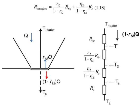
A description of the series of thermal conductances of the probe-sample is presented in Figure 1.8. Rs = 1/Gs is the spreading resistance in the sample where section 1.4 is dedicated to

present the modeling of this resistance in its different configurations. The heat mechanisms that operate between the probe and the sample are featured in Gc. Depending on the

description of the heat source and on the sample (bulk, layered samples …), different expressions of Gs can be used. We will present more in detail these two thermal conductances

later in this chapter.

Figure 1.8. Description of the network of the thermal conductances of the probe-sample system.

Let m²=hp/λS and Ω=Geq/Gp where Gp=λS/L is the probe thermal conductance. Solving

Equation (1.2) with the two conditions (Equations (1.3) and (1.4)), the probe Joule power when in contact is 2 3 [2 ( ) ( )] 2 2 [ 4 ( ) 2 ( )] [4(1 ( )) ( )] 2 2 2 2 c mL mL SL m mLch sh P mL mL mL mL mL sh mLch ch mLsh λ θ + Ω = − + + Ω − + (1.6)

And when out of contact is

2 3 2 ( ) 2 2 ( ) 4 ( ) 2 2 a mL SL m ch P mL mL mLch sh λ θ = − (1.7)

The expression P Pc Pa

P_c P_c

− ∆ ₌

was used in the calibration of SThM probes for the

measurements of the thermal conductivity of bulk samples [14, 23, 24]. In these works, the heat losses through convection were not taken into account (h=0). Under this condition, the resolution of Equation (1.2) leads to:

3 4 4( ) G G P _{c s} P_c G G_{p s} G G_{p c} G G_{c s} ∆ ₌ + + (1.8)

Later in this manuscript, we will show to what extent the coefficient h could affect the determination of the thermal conductivity of bulk samples and the thermal interaction parameters between the probe and the sample.

b) Alternating regime

When an AC current (alternating current) I=I0 cos(ωt) heats the probe, the Joule power

dissipated in the Pt/Rd wire is:

2 0 _{(1 cos(2 t))} 2 p RI P = + ω (1.9) Then, the temperature in the probe is:

2

( )t _{DC ω}cos(2 t )

θ =θ +θ ω φ+ (1.10) The probe voltage can be written as follows:

0 0 2 0 0 2

0(1 ) 0cos( t) cos( ) cos(3 t )

2 2

p DC

R I R I

V =RI =R +aθ I ω + β θ ω ω φt+ + β θ ω ω φ+ (1.11) Under the assumption that the other voltage harmonics are negligible.

Practically, the terms at the first harmonic are deliberately suppressed using a Wheatstone bridge since they are much larger than the terms at the third harmonic

0 0 2

3 cos(3 t )

2

R I

V_ω =RI = β θ ω ω φ+ . Through this expression, the alternating temperature θ2ω

can be experimentally determined. Through a proper modeling, this temperature can be related to the thermal properties of the sample. This method was first developed by Cahill (well-known 3ω method) [25] and was adapted by Lefèvre [22] to the Wollaston wire probe in the AC regime. For sake of simplification, the complex writing is used (I =I e₀ i tω ) and the temperature in the probe is written as:

2 2 ( )t _{DC ω}e i tω

θ =θ +θ (1.12) Then the heat equation in the alternating regime becomes [22]:

2 2 0 2 2 2 2 2 2 2 I i hp a S S x ω ω ω ρ θ ω θ θ λ λ ∂ = − + ∂ (1.13)

The same conditions in Equations (1.3) and (1.4) are used here for the resolution of Equation (1.13): 2 0 2 3 2 2 2 2 [ 1] [1 ] eq eq mL mL eq eq AG BG mL I Lm S e G e G mL ω ρ θ λ + = − + + (1.14) where 2 2 2 4 mL 2 mL mL A= − −mL+ e − e +mLe (1.15) and 2 2 1 mL mL B= +mL e− +mLe (1.16)

Parameters identified with these approaches:

Measuring θ_2ω through the measurements of V_3ω as a function of the angular frequency ω permits a determination of the equivalent conductance Geq for a specific sample [26]. Thus,

with appropriate description of the sample conductance Gs, one can determine the contact

conductance Gc for a sample of well-known thermal conductivity. This cannot be done in the

DC regime where the determined Gc is equivalent among different samples of well-known

thermal conductivity. However, an issue concerning the thermal expansion of the probe while working under the AC regime was reported [27]. In fact, the contact between the probe and the sample is not stable. That could be the reason behind the dispersion of the measurements obtained by Lefèvre [26].Based on these observations, Chapuis [27] suggested that it is better using the DC regime for distances of separation ds smaller than 50 nm.

1.4.2 The palladium probe

Puyoo [28] used the old palladium probe (with SiO2 cantilever) in the AC regime to determine

the thermal conductivity of silicon nanowires embedded in silicon dioxide sample. In his approach of measurement, he adapted the model of Lefèvre [24] to the palladium probe by describing the probe as two thermal fins composed of two adjacent materials (Pd and SiO2) as