Influence of dual conduit structure on solute transport in karst tracer tests: An experimental laboratory study

HAL Id: hal-02926746

https://hal.archives-ouvertes.fr/hal-02926746

HAL is a multi-disciplinary open access archive for the deposit and dissemination of sci-entific research documents, whether they are pub-lished or not. The documents may come from teaching and research institutions in France or abroad, or from public or private research centers.

L’archive ouverte pluridisciplinaire HAL, est destinée au dépôt et à la diffusion de documents scientifiques de niveau recherche, publiés ou non, émanant des établissements d’enseignement et de recherche français ou étrangers, des laboratoires publics ou privés.

Chaoqi Wang, Xiaoguang Wang, Samer Majdalani, Vincent Guinot, Hervé

Jourde

To cite this version:

Chaoqi Wang, Xiaoguang Wang, Samer Majdalani, Vincent Guinot, Hervé Jourde. Influence of dual conduit structure on solute transport in karst tracer tests: An experimental laboratory study. Journal of Hydrology, Elsevier, 2020, 590, pp.125255. �10.1016/j.jhydrol.2020.125255�. �hal-02926746�

Influence of dual conduit structure on solute transport in karst tracer tests: an experimental laboratory 1

study 2

Chaoqi Wang1_{, Xiaoguang Wang}1_{, Samer Majdalani}1_{, Vincent Guinot}1_{, Herve Jourde}1 3

1. Hydrosciences Montpellier, UMR 5569, France 4

Abstract 5

We conducted lab-scale experiments to investigate the mechanism of dual-peaked breakthrough curves (BTCs) 6

in karst tracer tests. Three groups of dual conduit structures were constructed by varying: (1) the length ratio between 7

the two conduits for a fixed length of the shorter conduit, (2) the total length of the conduits for a fixed length ratio, 8

(3) the connection angle between the conduits. The BTCs generated by the tracing experiments were fitted by a Dual-9

Region Advection Dispersion (DRAD) model to derive effective transport parameters. 10

Our results confirm that the dual conduit structure triggers the double-peaked BTCs. Increasing the conduit 11

length for a fixed length ratio or increasing the length ratio increases peak separation. The connection angles between 12

the two conduits θ1 and θ2 also influence the BTCs: increasing θ1 and decreasing θ2 causes the first peak to get smaller 13

and the second peak to get larger. The DRAD model can reproduce the dual-peaked BTCs while its application to 14

the case of single-peaked BTCs may be problematic due to strong interaction between model parameters. A method 15

is proposed for estimating underground karstic conduit lengths from experimental dual-peaked BTCs. 16

Keywords: karst conduit; tracer test, laboratory experiment; breakthrough curve; MCMC 17

Highlights: 18

1. The effect of dual conduit structure on solute transport is investigated using lab experiments 19

2. Increasing length ratio or total conduit length cause larger separation of dual peaks of BTCs 20

3. The connection angle affects tracer partition to the two conduits 21

4. A method for estimating the length of subsurface karst conduits based on BTCs is proposed 22

1. Introduction

The methodology of tracer test initially developed for the investigation of karst aquifers is still widely used in 24

karst hydrogeology. Tracer tests can provide information about groundwater trajectories and yield breakthrough 25

curves (BTCs) that can be used to estimate transport model parameters (Goldscheider and Drew, 2007). 26

Due to the strong heterogeneity of karst aquifers, the BTCs may exhibit asymmetry with long tails or multiple 27

peaks (Moreno and Tsang, 1991; Hauns et al., 2001; Massei et al., 2006; Perrin and Luetscher, 2008, Goldscheider 28

et al., 2008). The Advection–Dispersion-Equation (ADE) performs poorly in characterizing these BTCs. To better 29

reproduce tailing effects, some researchers considered including further processes in the transport model (Morales et 30

al., 2010): the Mobile-Immobile Model (MIM) developed by van Genuchten and Wierenga (1976) partitions the 31

aquifer into mobile and immobile regions; Skopp et al. (1981) proposed a dual-permeability model (also referred to 32

as the Multiple Region Advection-Dispersion (MRAD) by Majdalani et al. (2018)) with two mobile regions using 33

the ADE model. Berkowitz et al. (2006) proposed the Continuous Time Random Walk (CTRW) theory by 34

conceptualizing solute transport as a series of particle jumps or transitions with spatially changing velocities, recently 35

CTRW was also applied to karst aquifers (Goeppert et al., 2020). Dual-peaked BTCs were successfully modeled by 36

the application of the Dual Advection Dispersion Equation (DADE) and the Weighted Sum Advection-Dispersion 37

Equation (WSADE) model (Field and Leij, 2012). 38

Dual-peaked BTCs in karst tracer tests may be caused by the presence of pools (or underground lakes) along 39

main conduits (Field and Leij, 2012; Dewaide, 2018) or multiple flow paths (Maloszewski et al., 1992; Goldscheider 40

et al., 2008; Perrin and Luetscher, 2008). This hypothesis has been investigated using laboratory scale experiments 41

in the past (Moreno and Tsang, 1991; Field and Leij, 2012). Among the different experiments used for a better 42

understanding of karst aquifer solute transport, some scale models account for both the conduit and the matrix (Florea 43

and Wicks, 2001; Li et al., 2008; Mohammadi et al., 2019), while others focus on transport in conduits only (Zhao et 44

al., 2017, 2019; Field and Leij, 2012). Field and Leij (2012) noted that the presence of pools or auxiliary conduits 45

causes dual-peaked BTCs. Mohammadi et al. (2019) studied how the hydraulic head gradient influences BTCs by a 46

bench-scale karst model. Zhao et al. (2017, 2019) found that the existence of pools on the conduit would increase the 47

tailing of BTCs. However, these studies did not show whether karst conduit properties can be inferred from BTC 48

shapes. 49

To better assess the relationship between conduit structure and BTCs, we studied how the dual conduit geometry 50

influences the BTCs shape by laboratory tracer experiments. Three groups of solute transport experiments were 51

carried out. The obtained BTCs were fitted using a one-dimensional transport model to achieve a quantitative 52

comparison. 53

2 Materials and methods 54

2.1

Experimental setup

55

A series of lab-scale, idealized dual conduit structure models were built using silicone pipes with an internal 56

diameter of 0.4 cm. The dual conduit structure consists of three parts: the inlet, dual conduit and outlet. At the inlet 57

and outlet parts, the flow is restricted in the single conduit; at the dual conduit part, the flow is divided into two 58

conduits of different lengths (Fig. 1). The shorter and the longer conduit lengths are denoted as l1 and l2, respectively. 59

The deviation angles between the shorter and longer conduits at both the inlet and outlet connecting partare denoted 60

respectively as θ1 and θ2. During the experiments, the dual conduit structure is placed on a horizontal platform to 61

eliminate gravity effects. 62

63

Figure 1. Schematic diagram showing the experimental setup used in the study. 64

The inflowing flow is supplied using a peristaltic pump (Lead Fluid brand) at a constant rate. The discharge Q 65

is set at 0.6846 cm3_{/s, and hence the calculated velocity through the outlet conduit is 5.4480 cm/s. The inlet is} 66

connected in parallel to a pure water supply and a salty water supply. A three-way adapter is used to switch between 67

the salty water and pure water. The salty water (deionized water + NaCl at C0 = 0.06 mol/L) is used as the tracer. A 68

pulse tracer release is realized by switching the adaptor to the salty water supply for 5 seconds (3.42 mL). The 69

physical models were fully sealed and the recovery rate was 100% for all of the experiments. 70

We use a scale (Mettler ToledoTM_{) to estimate the discharge. A conductimeter (WTW TetraCon 325}TM_{, accuracy} 71

is 1×10-6 _{mol/L), is used to measure the outlet tracer concentration. The scale and conductimeter are connected to a} 72

data logger (Campbell CR1000TM_{) for automatic data recording at a time step of 1 second (In order to obtain more} 73

accurate peak time, the BTCs have been interpolated by 0.05 s.). In each experiment, the tracer injection is initiated 74

after the flow within the system is stabilized. Each experiment is repeated three times. A mean BTC is derived from 75

the replicates to reduce the measurement error. 76

Three groups of experiments are performed (Table 1). The notation for the experiment name takes the format of 77

l1 - l2 - θ1 - θ2 (Fig. 1). Experiment Group 1 is designed to study the effect of length ratio of the two conduits on the 78

transport process. l1 is set at 10 cm, while l2 is set to 20 cm, 40 cm, 60 cm, and 120 cm, respectively. The angles θ1 79

and θ2 are both fixed at 30 degrees. Experiment Group 2 is designed to study the effect of total conduit length variation 80

on the transport process, keeping the length ratio of two conduits as 1:6. l1 is set to be 10 cm, 20 cm and 60 cm and 81

l2 is set to be 60 cm, 120 cm, and 360 cm, respectively. The angles θ1 and θ2 of the connectors are also fixed at 30 82

degrees. Experiment Group 3 is designed to study the effect of the conduit connection angle on the transport process. 83

l1 is set at 10 cm and l2 is 60 cm, and three different connection types are made by arranging the θ1 and θ2 combinations. 84

In total, eight tracer tests are presented (the 10-60-30-30 experiment is used in all of the three groups as a reference 85

case). 86

Table 1. Geometrical parameters of dual conduit structures for the three groups of experiments 87 Group Experiment label Conduit length (cm) Connection angles (deg) l1 l2 θ1 θ2 1 10-20-30-30 10 20 30 30 10-40-30-30 10 40 30 30 10-60-30-30 10 60 30 30 10-120-30-30 10 120 30 30 2 10-60-30-30 10 60 30 30 20-120-30-30 20 120 30 30 60-360-30-30 60 360 30 30 3 10-60-30-120 10 60 30 120 10-60-30-30 10 60 30 30 10-60-120-30 10 60 120 30

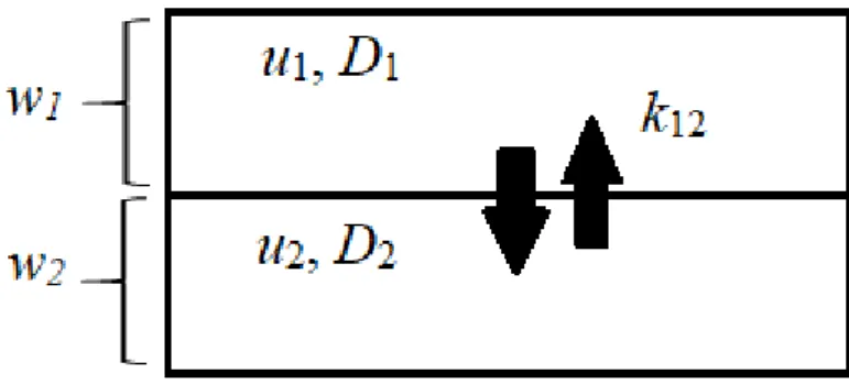
2.2 One-dimensional modeling 88

2.2.1 Dual Region Advection Dispersion (DRAD) model 89

To quantitatively investigate the dual-peaked BTCs obtained in section 2.1, we apply a Dual Region Advection 90

Dispersion (DRAD) model. This model has been called Two-Region MRAD model by Majdalani et al. (2018) and 91

DADE model by Field and Leij (2012). DRAD model assumes two regions flowing in parallel and exchanging mass 92

due to concentration difference; in both regions, the ADE model is assumed valid (Fig. 2). We do not consider solute 93

degradation or adsorption/desorption in our model. The DRAD model is chosen because it is the possible simplest 94

model to reproduce the dual-peaked BTCs. 95

The governing equations are given as follows: 96 2 2 ( ) ij i i i i i j i i k C C C u D C C t x x w  _  _  _{ }    , (i = 1, 2; j = 2, 1), (1) 97 k12 = k21, (2) 98 w1 + w2 = 1. (3) 99

The total concentration at the outlet is computed as: 100

 

 

 

C x t w C x t w C x t , (4)

101

where t is time (T), x is distance (L), Ci is the concentration (ML-3) of region i, ui, Di and wi are respectively the flow

102

velocity (LT-1_{), dispersion coefficient (L}2_T-1_{) and volumetric fraction in region i, k}

ij is the coefficient for solute

103

exchange between regions i and j (T-1_{). Since we consider only two-region systems, k}

12 = k21, and w1 + w2 = 1. As a 104

result, six independent parameters are involved in the calibration: w1, k12, u1, u2, D1 and D2. In our discussions, the 105

fast and slow regions are denoted by region 1and region 2 respectively (i.e., u1 > u2). 106

107

Figure 2. Schematic diagram of the DRAD model. 108

2.2.2 DRAD model parameter estimation 109

The six independent DRAD model parameters were estimated using the MCMC method (Haario et al., 2006). 110

The MCMC method is a Bayesian approach that evaluates the posterior distributions of parameters for an assumed 111

error structure (Vrugt et al., 2006). Using the Bayes rule, the probability density function of the model parameter set 112

θ={w1, k12, u1, u2, D1, D2} is given as: 113

𝑝(𝜽|𝐘) ∝ 𝐿(𝜽|𝐘) ∙ 𝑝(𝜽), (5) 114

where 𝑝(𝜽) and 𝑝(𝜽|𝐘) are the prior and posterior parameter distribution, respectively, 𝑌 = {𝑦(𝑡₁), … , 𝑦(𝑡𝑛)} is

115

the observations, 𝐿(𝜽|𝐘) is the likelihood function. The prior distribution 𝑝(𝜽) is assumed to follow a uniform 116

distribution. The model residual for outlet concentrations are assumed to be independent and follow a Gaussian 117

distribution with zero mean and a constant variance 𝜎2_{. Thus, the posterior distribution is given by:}

118 𝑝(𝜽|𝐘, 𝜎2) ∝ 1 (2𝜋𝜎2₎𝑁 2⁄ exp⁡(− ∑ (𝐶𝑛𝑖 𝑖−𝑌𝑖)2 2𝜎2 ), (6) 119

where N is the number of observations, Ci and Yi are the simulated and observed concentrations time i. The

120

convergence performance of MCMC chains is evaluated with a Root-Mean-Square-Error (RMSE) objective function, 121

which is defined as: 122

𝑅𝑀𝑆𝐸 = √∑𝑛𝑖=1(𝐶𝑖−𝑌𝑖)2

𝑁 . (7)

We used the Metropolis-Hastings (MH) algorithm to successively draw samples from the posterior distribution 124

by forming a Markov chain of model parameter set 𝜽. The MH algorithm constructs a Markov chain in four main 125

steps: (1) choose an initial parameter set 𝜽0 _{and a proposal density distribution 𝑞(𝜽}

𝑘|𝜽𝑘−1); (2) at each iteration k

126

+ 1, generate a new sample 𝜽∗ _{from 𝑞(𝜽}∗_|𝜽𝑘_{) and calculate the probability of acceptance, 𝜋 =}

127

min (𝑝(𝜽

∗_)𝐿(𝜽∗_{|𝐘)𝑞(𝜽}𝑘_|𝜽∗₎

𝑝(𝜽𝑘)𝐿(𝜽𝑘|𝐘)𝑞(𝜽∗|𝜽𝑘)

, 1), draw a random number u from a uniform distribution between 0 and 1; (3) if 𝜋 > 𝑢, 128

set 𝜽𝑘+1 _{= 𝜽}∗_{; otherwise 𝜽}𝑘+1_{= 𝜽}𝑘_{; (4) repeat steps 2 and 3 until a given maximum number of iteration is reached.}

129

To achieve a fast convergence of the chain, we first perform a manual fitting of the DRAD response to the 130

experimental BTCs to find the initial parameter set. In this work, we assume the posterior distribution is Gaussian. 131

For each chain, 16000 iterations are executed, and the last 1000 sampled parameter sets that allow the model to 132

adequately fit the observed data were chosen to evaluate the posterior parameter distribution and the pairwise 133

parameter correlations. Except for 10-20-30-30, all of the fitted parameters are set to be the mean value of these 1000 134

sets. For 10-20-30-30, the fitted parameters are chosen with the criterion: w1 > 0.5. 135

The parameter correlations are characterized by scatterplots of parameter pairs and the correlation coefficient r, 136

which is a statistical measure of the linear relationship between two variables. Given paired data {(x1, y1), (x2, y2), …, 137 (xn, yn)}, r is defined as: 138





















where n is the sample size; 𝑥̅ and 𝑦̅ are the mean value for x and y, respectively. The parameter variability (or 140

uncertainty) is represented by the parameter histogram and relative standard deviation (RSD) value. RSD is calculated 141 by: 142







3. Results

3.1 Length ratio study (experiment Group 1)

145

The BTCs from Experiment Group 1 (Fig. 3) trigger the following observations. When the length ratio is small 146

(e.g., 2), the BTC only exhibits a single peak; for length ratio of 4, 6 and 12, the BTCs exhibit two peaks. As the 147

length ratio increases, the first peak arrives slightly earlier while the arrival of the second peak is delayed. The value 148

of the first peak (Cpeak1) decreases first from the 10-20-30-30 to the 10-40-30-30 case and then increases as the length 149

ratio is further increased. The concentration value of the second peak (Cpeak2) decreases as the length ratio increases. 150

Using the DRAD model and the MCMC calibration algorithm, we try to correctly fit the experimental BTCs. 151

Visually the simulated BTCs can capture the main shape of the experimental BTCs. The overall fitting performance 152

is quite good for the 10-40-30-30 system with a maximum error value of 0.0233 (Table 2). However, the recession 153

limb of the second peak of some experimental BTCs (Fig. 3b, c) exhibits a slight skewness, which the DRAD model 154

is unable to capture exactly (Fig. 3b, c, d). For the first experiment (Fig. 3a), the DRAD model allows a good fit for 155

the BTC curve. For the dual-peaked BTCs (Fig. 3b, c), the fit of the second peak is not as good as the fit of the first 156

peak but the overall BTC behavior is correctly reproduced by the DRAD model. The parameters of the fitting result 157

for Group 1 are listed in Table 2 and plotted in Figure 4. We do not plot the variation of the exchange rate k12 because 158

of the very small values that indicate a negligible exchange rate and therefore a negligible effect on the BTC. 159

160

Figure 3. DRAD calibration results of Group 1 experiments. 161

Table 2. DRAD model calibration results for Group 1 experiments 162 10-20-30-30 10-40-30-30 10-60-30-30 10-120-30-30 tpeak1 (s) 6.45 4.85 4.55 4.40 tpeak2 (s) 6.45 17.20 27.85 73.00 u1 (m/s) 4.46×10-2 5.04×10-2 5.13×10-2 5.09×10-2 u2 (m/s) 1.89×10-2 9.40×10-3 5.27×10-3 1.46×10-3 u1 (m/PV) 3.17×10-1 5.43×10-1 7.41×10-1 1.29×100 u2 (m/PV) 1.34×10-1 1.01×10-1 7.61×10-2 3.71×10-2 D1 (m2/s) 5.71×10-4 3.99×10-4 7.42×10-4 1.05×10-3 D2 (m2/s) 3.86×10-4 4.03×10-5 1.82×10-5 1.47×10-5 k12 (1/s) 7.14×10-37 3.25×10-25 3.08×10-28 1.99×10-26 w1 (–) 0.526 0.562 0.632 0.653 RMSE (–) 0.00967 0.0233 0.0165 0.0120

163

Figure 4. Variation of fitted parameter values with experimental model length for Group 1 experiments. (a) 164

Velocities in the two regions, u1 and u2, (b) Dispersion coefficient of region 1, D1, (c) Dispersion coefficient of 165

region 2, D2, (d) Water content ratio of region 1, w1. 166

From Figure 4a, we find that, as the length ratio increases from 2 to 12, the velocity of region 1 (u1) increases 167

from 4.46×10-2 _{to 5.09×10}-2 _{(1:1.14). The major increase in u}

1 value occurs when transiting between 10-20-30-30 168

and 10-40-30-30 cases, while the u1 is only slightly increased from 10-40-30-30 to 10-120-30-30 cases.The velocity 169

of region 2 (u2) shows a significant decreasing trend, decreases from 1.89×10-2 to 1.46×10-3 (12.9:1) from 10-20-30-170

30 to 10-120-30-30 and u2 decreases from 9.40×10-3 to 1.46×10-3 (6.45:1) from 10-40-30-30 to 10-120-30-30. This 171

is consistent with the fact that from 10-40-30-30 to 10-120-30-30 the second peak gets increasingly delayed (Fig. 3). 172

As we can see from Figure 4b, the D1 value does not show any continuous increasing trend: as the ratio increases 173

from 2 to 12, D1 increases from 5.71×10-4 to 1.05×10-3 (1:1.84), and as the ratio increases from 4 to 12, D1 increases 174

from 3.99×10-4 _{to 1.05×10}-3 _{(1:2.63). Such behavior of D}

1 variation may be caused by the strong correlation between 175

some parameters for the case of 10-20-30-30 (see parameter identifiability results in Section 3.4 and discussion in 176

Section 4.3). As the ratio increases from 2 to 12, D2 decreases from 3.86×10-4 to 1.47×10-5 (2.73:1). As the ratio 177

increases from 2 to 12, w1 increases from 0.526 to 0.653 (1:1.24), w2 decreases from 0.474 to 0.347 (1.36:1). This is 178

in agreement with the trend observed from Figure 3 (except for the experiment 10-20-30-30, which only has one 179

peak): as the length ratio increases, the area below the second peak (A2), and, thus, the mass transported through the 180

longer conduit decreases. 181

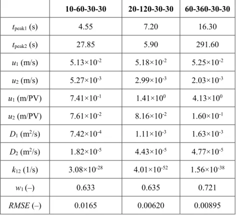
3.2 Total length study (experiment Group 2)

182

In this series of experiments, the length ratio is fixed to 6.0 and the total length (l1+l2) varies. The experimental 183

BTCs and the numerical fitting of Group 2 are shown in Figure 5. For Group 2, all of the tested dual conduit structures 184

exhibit double-peaked BTCs. As the length increases, the two peaks become increasingly separated. As the length 185

increases, both Cpeak1 and Cpeak2 show a decreasing trend, with Cpeak2 decreasing faster than Cpeak1. For the experiment 186

60-360-30-30, the longer conduit has a strong flow resistance. Thus, the amount of tracer that enters this conduit is 187

much less. As a result, the second peak has a very low concentration value (0.0148) and is hardly visible on the plot. 188

A visual inspection indicates that the DRAD does not equally capture the two peaks of the experimental BTCs. 189

Similar to the analysis of Group 1 results, the skewness of the second peak in the BTCs is not perfectly reproduced 190

by the DRAD model. The parameters of the fitting result are listed in Table 3. The fitted parameters for Group 2, 191

except the exchange rate k12 that remains negligible, are plotted in Figure 6. 192

Figure 5. DRAD calibration results for Group 2 experiments. 194

Table 3. DRAD model calibration results for Group 2 experiments 195 10-60-30-30 20-120-30-30 60-360-30-30 tpeak1 (s) 4.55 7.20 16.30 tpeak2 (s) 27.85 5.90 291.60 u1 (m/s) 5.13×10-2 5.18×10-2 5.25×10-2 u2 (m/s) 5.27×10-3 2.99×10-3 2.03×10-3 u1 (m/PV) 7.41×10-1 1.41×100 4.13×100 u2 (m/PV) 7.61×10-2 8.16×10-2 1.60×10-1 D1 (m2/s) 7.42×10-4 1.11×10-3 1.63×10-3 D2 (m2/s) 1.82×10-5 4.43×10-5 4.77×10-5 k12 (1/s) 3.08×10-28 4.01×10-52 1.56×10-38 w1 (–) 0.633 0.635 0.721 RMSE (–) 0.0165 0.00620 0.00895 196

197

Figure 6. Variation of fitted parameter values with experimental model length for Group 2 experiments. (a) 198

Velocities in the two regions, u1 and u2, (b) Dispersion coefficient of region 1, D1, (c) Dispersion coefficient of 199

region 2, D2, (d) Water content ratio of region 1, w1. 200

As shown in Figure 6. As the length increases from 10cm-60cm to 60cm-360cm (1:6), the velocity u1 increases 201

from 5.13×10-2 _{to 5.25×10}-2 _{(1:1.02), and u}

2 decreases from 5.27×10-3 to 2.03×10-3 (2.60:1) (Fig. 6a). The dispersion 202

coefficient of both regions increases: D1 increases from 7.42×10-4 to 1.63×10-3 (1:2.19), D2 increases from 1.82×10 -203

5 _{to 4.77×10}-5 _{(1:2.62), (Fig. 6 b, c). w}

1 remains almost the same, from 0.633 to 0.721 (1:1.14), (Fig. 6d). 204

3.3 Connection angle (experiment Group 3)

205

For Group 3 experiments (Fig. 7), the connector angle between two conduits has an important influence on the 206

flow and transport process. As the (θ1-θ2) value increases, the two peaks become closer to each other; Cpeak1 decreases, 207

Cpeak2 increases. 208

Same with previous groups, the fit is better for the first peak of the experiment BTCs than for the second peak, 209

with a maximum error value to be 0.0168 (Table 4). The fitted parameters for Group 3 are plotted in Figure 8. 210

211

Figure 7. DRAD calibration results of Group 3 experiments. 212

Table 4. DRAD model calibration results for Group 3 experiments 213 10-60- 30-120 10-60- 30-30 10-60- 120-30 (θ1-θ2) (deg) -90 0 90 tpeak1 (s) 4.40 4.55 6.15 tpeak2 (s) 39.65 27.85 17.60 u1 (m/s) 5.39×10-2 5.13×10-2 2.99×10-2 u2 (m/s) 3.31×10-3 5.27×10-3 8.56×10-3 u1 (m/PV) 7.78×10-1 7.41×10-1 4.32×10-1 u2 (m/PV) 4.78×10-2 7.61×10-2 1.24×10-1 D1 (m2/s) 7.81×10-4 7.42×10-4 3.55×10-4 D2 (m2/s) 2.22×10-5 1.82×10-5 3.17×10-5 k12 (1/s) 6.33×10-34 2.19×10-33 9.28×10-26 w1 (-) 0.732 0.633 0.451

RMSE (-) 0.0131 0.0165 0.0168

214

Figure 8. Variation of fitted parameter values with experimental model length for Group 3 experiments. (a) 215

Velocities in the two regions, u1 and u2, (b) Dispersion coefficient of region 1, D1, (c) Dispersion coefficient of 216

region 2, D2, (d) Water content ratio of region 1, w1. 217

Figure 8a shows that as (θ1 - θ2) increases from -90° to 90°, u1 decreases from 5.39×10-2 m/s to 2.99×10-2 m/s 218

(i.e., by 1.8 times) and u2 increases from 3.31×10-3 m/s to 8.56×10-3 m/s (~ 2.6 times). This conforms to the fact that 219

as (θ1-θ2) increases, the first peak is delayed and the second peak appears sooner (Fig. 7). The D1 decreases from 220

7.81×10-4 _m2_{/s to 3.55×10}-5 _m2_{/s (~ 2.2 times) (Fig. 8b); the D}

2 increases from 2.22×10-5 m2/s to 3.17×10-5 m2/s (~ 221

1.4 times) (Fig. 8c). w1 decreases from 0.732 to 0.451 (~ 1.6 times) while w2 increases from 0.268 to 0.549 (~ 2 times) 222

(Fig. 8d). The changes in w1 and w2 values are consistent with a smaller first peak and a larger second peak (Fig. 7). 223

3.4 Parameter identifiability

224

As presented in section 3.1, the variation of the estimated parameter set for the 10-20-30-30 experiment does 225

not show a trend consistent with that of other experiments. We thus perform a study to check the identifiability of 226

model parameters for various Group 1 experiments based on the statistics extracted from respective MCMC chains. 227

The priori distribution of DRAD parameters used in the MCMC calibration of the two experiments is shown in Table 228

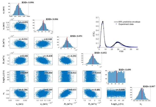
5. Figures 9 and 10 present the MCMC statistics for the 10-20-30-30 and 10-60-30-30 experiments, respectively. The 229

on-diagonal plots of these figures are the estimated posterior parameter distributions for each parameter, while the 230

off-diagonal plots correspond to scatterplots between parameter pairs. A widespread point cloud on the scatterplots 231

indicates that the parameters are independent. A narrow stripe on the scatterplots means a strong correlation between 232

two parameters. The correlation intensity is quantified by the correlation coefficient r (as defined by Eq. 8), which is 233

indicated in the scatterplots. The 95 percentiles of the breakthrough curves are shown in the inset above the diagonal. 234

Figure 9. MCMC solutions to the experiment of 10-20-30-30. 236

237

Figure 10. MCMC solutions to the experiment of 10-60-30-30. 238

Table 5. A priori distribution of DRAD parameters used in the MCMC calibration 239

Initial input Range

Distribution 10-20-30-30 10-60-30-30 Min Max u1 (m/s) 3.04×10-2 5.50×10-2 u1×0.005 u1×200 Uniform u2 (m/s) 1.60×10-2 5.30×10-3 u2×0.005 u2×200 Uniform D1 (m2/s) 8.71×10-4 9.30×10-4 0 500×D1 Uniform D2 (m2/s) 6.00×10-6 1.82×10-5 0 500×D2 Uniform k12 (1/s) 4.50×10-8 4.50×10-8 1.00×10-100 1.00×10-5 Uniform w1 (–) 0.5 0.6325 0.01 0.99 Uniform

It can be seen that except for k12, all other parameters are appropriately identified as their posterior distribution 240

is Gaussian (Fig. 9). In a simple sensitivity test, we observe that varying k12 within a wide range between 10-90 and 241

10-8 _{and fixing all other parameters, there is no change in the outlet breakthrough curve. Changes in breakthrough} 242

curves only occur when k12 takes a large value, which is on the magnitude of 10-3. This means that the model is 243

insensitive to k12 as long as its value is small. 244

For the other parameters, the 10-20-30-30 experiment exhibited a strong interaction between parameters (Fig. 245

9). According to the parameter correlation plots, we find some parameter pairs, for example, u2-D2, u2-w1 and D2-w1, 246

even exhibited a linear trend on the cross plot. The strong correlations are also shown by the high values of correlation 247

coefficients |r| (nearly equal to 1; Fig. 9). The other parameter pairs like u2-D1, D1-D2 and D1-w1 exhibited a slightly 248

lower correlation strength, with |r| values of 0.748, 0.712 and 0.772. 249

In contrast, the 10-60-30-30 experiment exhibited stronger parameter identifiability and much weaker parameter 250

interaction (Fig. 10). No obvious correlation between the parameters was found. The maximum |r| value of 0.611 251

was found for the parameter pair D1-w1. The variation range of posterior distributions of the parameters was also 252

smaller. The dispersion coefficients, D1 and D2, have the largest RSD values of 0.051 and 0.052, respectively. The 253

RSD values of other parameters such as u1, u2, w1 are quite small, i.e., 0.006, 0.006, 0.007, respectively. These 254

observations indicate the DRAD model parameters were properly identified for the 10-60-30-30 experiment. Similar 255

behavior has also been found for other experiments (not shown here) with larger conduit length ratios. 256

4. Discussion

4.1 Representativeness of the experiments for karst tracer tests

258

We examine to which degree our experiments are representative of natural karst systems and the possibility to 259

extrapolate our laboratory finding to the characterization of karst aquifers based on field tracer tests. We calculate 260

three dimensionless quantities (i.e., the conduit length to diameter ratio, Péclet number and Reynolds number) to 261

evaluate the geometric, kinematic and dynamic similarities between our experiments and previous field studies (Table 262

6, see also Appendix A for a summary of parameter values reported in the literature). The Péclet number Pé is a 263

measure of the relative importance of advection versus diffusion. It is defined as: 264

Pé Lu

D

 , (10)

265

where L is the characteristic length (L), u is the local flow velocity (LT-1_{), D is the diffusion coefficient (L}2_T-1_{). The} 266

Reynolds number Re is the ratio of inertial forces to viscous forces within a fluid: 267 Re ud   , (11) 268

where



is the dynamic viscosity of the fluid (ML-1_T-1_). 270

The range of values of the geometric and kinematic similarity criteria (i.e., the conduit length-diameter ratio and 271

Péclet number) of our experiments fall within the range of values obtained under field conditions. Regarding the 272

dynamic similarity criterion, the Reynolds number of our experiments is quite small compared to that obtained from 273

field tracer tests. In our experiments, the fluid flow in conduits is laminar (i.e., Re < 2000), while it is well known 274

that the turbulent flow often occurs in natural karst aquifers. Although the difference in flow regime may induce a 275

discrepancy in pressure or flow rate in the conduits, the general trend that the flow rate is positively correlated to the 276

hydraulic head gradient is still respected. Thus, the observed effect of conduit geometry on transport responses may 277

still provide important insights for the interpretation of field tracer tests in natural karst systems. 278

Table 6. Comparison of dimensionless quantities between published field data and our experiments 279

Similarity criterion

Dimensionless number Range of

Values in nature (karst tracer tests) Range of Values for the experiment Geometry Conduit length to

diameter ratio

l d

25-25000 37.5-162.5

Kinematic Péclet number Lu

D

12-331 7.77-21.27

Dynamic Reynolds number

ud





6500-87000 144

Our experimental work confirms that the dual conduit structure generally results in dual-peaked BTCs, as 280

shown in previous studies (Smart, 1988; Perrin and Luetscher, 2008; Field and Leij, 2012). We further found that the 281

number of peaks in the BTCs is not necessarily the same as the number of conduits when the length of the two 282

conduits is similar. For example, the BTC of experiment 10-20-30-30 showed only one peak. The single peak is 283

composed of two overlapping concentration fronts, whose arrival times to the outlet are similar. 284

4.2 Inferring conduit lengths from dual-peaked BTCs 285

We propose to use tracer BTCs to infer the length of conduits that form a looped network as shown in Figure 1 286

and Figure B1. For dual-peaked BTCs, we denote the areas below the first and second peaks by A1 and A2 respectively. 287

For cases where the two peaks are fully separated, A1/A2 may be used to approximate the ratio of the tracer amount 288

of the two conduits. When the Péclet number is sufficiently high (as in our experiments, Pé ranges from 7.77 to 289

21.27), advection dominates the flow process. The flow rate ratio between the conduits may thus be approximated 290

with the ratio of tracer amount passing through the two conduits, i.e., Q1/Q2 ≈ A1/A2 (see Appendix B for details). The 291

mean travel times of the two packs of tracer at the outlet may be estimated by the concentration peak times tpeak1 and 292

tpeak2. If all conduits are assumed to have a constant diameter, that may be estimated by field investigations, by 293

applying mass conservation at the diverging and converging points of the dual-conduit network, the length of the 294

shorter and longer conduits can be estimated by: 295









where l1e and l2e, are respectively the estimated lengths of the shorter and longer conduits; L is the total length of the 298

dual-conduit structure, i.e., the distance from the injection point to the sampling point via the shorter conduit, Sf is 299

the sinuosity factor, R is the conduit radius, Q1 and Q2 are respectively the flow rates of shorter and longer conduits. 300

We validate the proposed method for estimating lengths of subsurface conduits by applying it to our 301

experimental data of Groups 1 and 2. The ratios between the estimated length and the actual length for the two 302

conduits, l1e/ l1 and l2e/ l2 are shown in Figure 11. It can be seen that the length ratios for various experiments scatter 303

around 1.0, which indicates an effective estimation. The average value of this ratio is 1.058, the estimated values tend 304

to be slightly larger than the true value. The shorter conduit length seems better identified than that of the longer 305

conduit. This may be caused by the stronger skewness of the second peak (i.e., stronger dispersion in the longer 306

conduit). The most biased case is the 10-60-30-120 experiment, where the ratio for the shorter conduit, l1e/ l1 = 1.20. 307

However, the ratio is still very close to 1.0. This indicates that the proposed method is valid at least for the tested 308

conduit network configurations and flow conditions. It is stressed that the method is based on the assumption the 309

conduit diameter is constant for the entire system and is known. The geometrical complexity of natural karst system 310

may invalidate the assumption and imply considering an equivalent conduit diameter. Obviously, the method should 311

be checked for the more general cases of variable conduit diameter when experimental data for such experiments 312

become available. 313

The method is applicable when BTCs show fully separated dual peaks. Its usage may be hindered if the two 314

peaks overlap each other. For instance, in the interpretation of the BTCs of the 10-40-30-30 and 10-60-120-30 315

experiments, we used the local minimum concentration point between the two peaks to approximately separate them 316

and assess the areas under the two peaks. The results of estimated conduit lengths appear reasonably good. On the 317

other hand, the method is expected to be inaccurate when the two peaks are further separated. For example, in 318

Experiment 60-360-30-30, the small value of the second peak makes it difficult to evaluate A2 because the 319

concentration value is of the same order of magnitude as the background noise signal. For real karst tracer tests, the 320

low concentration signal is very possible to be hidden behind the background noise signals. This suggests us not to 321

ignore the low concentration signals when performing tracer tests in real karst aquifers. Because this low 322

concentration peak may indicate the existence of very long secondary conduits, through which a few quantities of 323

tracer is transported. 324

325

Figure 11. Calculated values of estimated to true conduit length ratio for various experiments. 326

4.3 Parameter identifiability of DRAD model 327

The distributions for the sets of parameters of 10-20-30-30 exhibited a strong interaction (u2-D1, D1-D2, D1-w1). 328

In the 10-20-30-30 experiment, the concentration fronts from the two flowing regions do not separate, i.e., the 329

concentration is similar at a certain time. On the other hand, solute migration in the two regions of DRAD is modeled 330

using two similar transport equations. Since the two transport equations have to handle similar concentration, it is 331

likely that the contribution of the two transport equations to the model responses is indistinguishable. However, it 332

should be noted that the issue of difficult to separate model parameters observed in our study is different from the 333

equifinality issue as discussed in Younes et al., (2016). Younes et al (2016) used a similar dual flowing continuum 334

model to examine transport problems in porous media that includes biofilm phases. The equifinality of their model 335

due to the non-separated concentration fronts in model responses results essentially from a high exchange rate 336

between the dual flowing phases. In contrast, in our experiments there is almost no mass exchange between the two 337

regions. The non-separation of concentration peaks results from the similar arrival times of two packs of solute travel 338

through the two conduits. 339

According to the RSD and r values, the fitting MCMC chain of 10-60-30-30 showed weaker interaction. The 340

DRAD showed different parameter identifiability for 10-20-30-30 and 10-60-30-30 data. One model may perform 341

good parameter identifiability when characterizing a given BTC and exhibits weak identifiability for another one. 342

This has been noted by previous studies (Wagner and Harvey, 1997; Kelleher et al., 2013; Rana et al., 2019). It seems 343

necessary to study the model parameter identifiability with more cases. 344

For the single-peaked BTC, the DRAD model may reproduce the curve sufficiently well but some of the 345

estimated parameters show strong correlations. This indicates that the DRAD is not optimally parsimonious for 346

single-peaked BTC. For the dual-peaked BTCs, DRAD can adequately characterize the dual-peaked BTCs on the 347

whole with good parameter identifiability, but does not characterize the skewness of the BTC peaks satisfactorily. 348

Finding an optimal model for all situations is beyond the scope of the present study and is left for future research. 349

Model fitting yields a negligible exchange rate k12. This is attributed to the difference between the conceptual 350

structure of the DRAD model and the physics of the transport process in the experiment. In the DRAD model, mass 351

exchange is assumed to take place along the entire model length, while in the experimental setup mass exchange only 352

occurs at the divergence and convergence between the two conduits. 353

5. Conclusion

In this paper, we studied the solute transport process in dual conduit structures by lab-scale experiments. The 355

main contributions of this study are summarized as follows. 356

First, we studied how the dual-conduit structure may influence the BTCs shape, specifically: 1) As the length 357

ratio increases, on the C-PV plot, the two peaks get more separated, the concentration value of the first peak (Cpeak1) 358

increases and the second peak (Cpeak2) decreases; 2) As the total length increases, the two peaks become increasingly 359

separated and the concentration value of both peaks decreases, while Cpeak2 decreases much more than Cpeak1; 3) As 360

the (θ1-θ2) value of the dual-conduit connection increases, the size of the first peak (A1), and thus the mass transported 361

through the shorter conduit, gets smaller and the size of the second peak (A2), and thus the mass transported through 362

the longer conduit, gets bigger. 363

Second, we proposed a method to estimate underground conduit length from recorded dual-peaked BTCs, 364

assuming a known average conduit diameter. The method exhibits good performance when applied to the 365

experimental BTCs. Whether the method applies to the interpretation of real karst tracer tests needs to be further 366

confirmed by fully controlled field experiments. 367

Third, we studied the ability of the DRAD model to reproduce BTCs with a single peak and double peaks. For 368

the single-peaked BTCs, the experimental data are well reproduced, but the low parameter identifiability indicates 369

that the DRAD model is non-optimally parsimonious. For dual-peaked BTCs, the DRAD model achieves a good 370

fitting with stronger parameter identifiability, although the exchange coefficient is consistently negligible. For some 371

experiments, the model fails to reproduce the skewness of some parts of the slower peaks. While it may be considered 372

useful for predictive purposes for a given site on which it has been properly calibrated, the analysis of the fitting 373

results shows that its parameters do not necessarily bear a physical meaning. A path for research thus focuses on the 374

development of models, the parameters of which would reflect the geometric and hydraulic reality of the experiments. 375

The following limitations are acknowledged for the present study: (i) the flow regime in the experiments is 376

laminar, while it can be turbulent in field tracer tests, (ii) structures with variable conduit diameter were not studied, 377

(iii) neither the influence of varying flow velocities. Studying the influence of such factors is the subject of ongoing 378

research. 379

Acknowledgments 380

C. W. is supported by the China Scholarship Council (CSC) from the Ministry of Education of P.R. China. X.W. and 381

H. J. are grateful for financial support from the European Commission through the Partnership for Research and 382

Innovation in the Mediterranean Area (PRIMA) program under Horizon 2020 (KARMA project, grant agreement 383

number 01DH19022A). 384

Reference

Berkowitz, B., Cortis, A., Dentz, M. and Scher, H., 2006. Modeling non-Fickian transport in geological 386

formations as a continuous time random walk. Reviews of Geophysics, 44(2). 387

Dewaide, L., Collon, P., Poulain, A., Rochez, G. and Hallet, V., 2018. Double-peaked breakthrough curves as a 388

consequence of solute transport through underground lakes: a case study of the Furfooz karst system, Belgium. 389

Hydrogeology journal, 26(2), pp.641-650. 390

Doummar, J., Margane, A., Geyer, T. and Sauter, M., 2012. Artificial Tracer Test 5A – June 2011. - Special 391

Report No. 6 of Technical Cooperation Project "Protection of Jeita Spring", Department of Applied Geology, 392

University of Göttingen, Germany & Federal Institute for Geosciences and Natural Resources (BGR), Germany. 393

Duran, L., Fournier, M., Massei, N. and Dupont, J.P., 2016. Assessing the nonlinearity of karst response function 394

under variable boundary conditions. Groundwater, 54(1), pp.46-54. 395

Field, M.S., 1999. The QTRACER program for tracer-breakthrough curve analysis for karst and fractured-rock 396

aquifers (Vol. 98). National Center for Environmental Assessment--Washington Office, Office of Research and 397

Development, US Environmental Protection Agency. 398

Field, M.S., 2002. The QTRACER2 program for tracer-breakthrough curve analysis for tracer tests in karstic 399

aquifers and other hydrologic systems. National Center for Environmental Assessment--Washington Office, Office 400

of Research and Development, US Environmental Protection Agency. 401

Field, M.S. and Leij, F.J., 2012. Solute transport in solution conduits exhibiting multi-peaked breakthrough 402

curves. Journal of Hydrology, 440, pp.26-35. 403

Florea, L.J. and Wicks, C.M., 2001. Solute transport through laboratory-scale karstic aquifers. 404

Geography/Geology Faculty Publications, p.11. 405

Goldscheider, N. and Drew, D., 2007. Methods in karst hydrogeology. International Contributions to 406

Hydrogeology, 26. 407

Goldscheider, N., Meiman, J., Pronk, M. and Smart, C., 2008. Tracer tests in karst hydrogeology and speleology. 408

International Journal of Speleology, 37(1), pp.27-40. 409

Göppert, N. and Goldscheider, N., 2008. Solute and colloid transport in karst conduits under low- and high-410

flow conditions. Groundwater, 46(1), pp.61-68. 411

Goeppert, N., Goldscheider, N. and Berkowitz, B., 2020. Experimental and modeling evidence of kilometer-412

scale anomalous tracer transport in an alpine karst aquifer, 115755. 413

Haario, H., Laine, M., Mira, A. and Saksman, E., 2006. DRAM: efficient adaptive MCMC. Statistics and 414

Computing, 16(4), pp.339-354. 415

Hauns, M., Jeannin, P.Y. and Atteia, O., 2001. Dispersion, retardation and scale effect in tracer breakthrough 416

curves in karst conduits. Journal of Hydrology, 241(3-4), pp.177-193. 417

Kelleher, C., Wagener, T., McGlynn, B., Ward, A. S., Gooseff, M. N., & Payn, R. A. (2013). Identifiability of 418

transient storage model parameters along a mountain stream. Water Resources Research, 49(9), 5290-5306. 419

Li, G., Loper, D.E. and Kung, R., 2008. Contaminant sequestration in karstic aquifers: Experiments and 420

quantification. Water Resources Research, 44(2). 421

Majdalani, S., Guinot, V., Delenne, C. and Gebran, H., 2018. Modeling solute dispersion in periodic 422

heterogeneous porous media: Model benchmarking against experiment experiments. Journal of Hydrology, 561, 423

pp.427-443. 424

Maloszewski, P., Harum, T. and Benischke, R., 1992. Mathematical modeling of tracer experiments in the karst 425

of Lurbach system. Steierische Beiträge zur Hydrogeologie, 43, pp.116-136. 426

Massei, N., Wang, H.Q., Field, M.S., Dupont, J.P., Bakalowicz, M. and Rodet, J., 2006. Interpreting tracer 427

breakthrough tailing in a conduit-dominated karstic aquifer. Hydrogeology Journal, 14(6), pp.849-858. 428

Mohammadi, Z., Gharaat, M.J. and Field, M., 2019. The Effect of Hydraulic Gradient and Pattern of Conduit 429

Systems on Tracing Tests: Bench-Scale Modeling. Groundwater, 57(1), pp.110-125. 430

Morales, T., Uriarte, J.A., Olazar, M., Antigüedad, I. and Angulo, B., 2010. Solute transport modelling in karst 431

conduits with slow zones during different hydrologic conditions. Journal of hydrology, 390(3-4), pp.182-189. 432

Moreno, L. and Tsang, C.F., 1991. Multiple-peak response to tracer injection tests in single fractures: A 433

numerical study. Water Resources Research, 27(8), pp.2143-2150. 434

Perrin, J. and Luetscher, M., 2008. Inference of the structure of karst conduits using quantitative tracer tests and 435

geological information: example of the Swiss Jura. Hydrogeology Journal, 16(5), pp.951-967. 436

Rana, S. M., Boccelli, D. L., Scott, D. T., & Hester, E. T., 2019. Parameter uncertainty with flow variation of 437

the one-dimensional solute transport model for small streams using Markov chain Monte Carlo. Journal of Hydrology, 438

575, pp.1145-1154. 439

Skopp, J., Gardner, W.R. and Tyler, E.J., 1981. Solute movement in structured soils: Two-region model with 440

small interaction. Soil Science Society of America Journal, 45(5), pp.837-842. 441

Smart, C.C., 1988. Artificial tracer techniques for the determination of the structure of conduit aquifers. 442

Groundwater, 26(4), pp.445-453. 443

Upchurch, S., Scott, T.M., ALFIERI, M., Fratesi, B. and Dobecki, T.L., 2018. The Karst Systems of Florida: 444

Understanding Karst in a Geologically Young Terrain. Springer. 445

Van Genuchten, M.T. and Wierenga, P.J., 1976. Mass transfer studies in sorbing porous media I. Analytical 446

solutions 1. Soil Science Society of America Journal, 40(4), pp.473-480. 447

Vrugt, J.A., Clark, M.P., Diks, C.G., Duan, Q. and Robinson, B.A., 2006. Multi-objective calibration of forecast 448

ensembles using Bayesian model averaging. Geophysical Research Letters, 33(19). 449

Wagner, B.J. and Harvey, J.W., 1997. Experimental design for estimating parameters of rate-limited mass 450

transfer: Analysis of stream tracer studies. Water Resources Research, 33(7), pp.1731-1741. 451

Younes, A., Delay, F., Fajraoui, N., Fahs, M. and Mara, T.A., 2016. Global sensitivity analysis and Bayesian 452

parameter inference for solute transport in porous media colonized by biofilms. Journal of Contaminant Hydrology, 453

191, pp.1-18. 454

Zhao, X., Chang, Y., Wu, J. and Peng, F., 2017. Laboratory investigation and simulation of breakthrough curves 455

in karst conduits with pools. Hydrogeology Journal, 25(8), pp.2235-2250. 456

Zhao, X., Chang, Y., Wu, J. and Xue, X., 2019. Effects of flow rate variation on solute transport in a karst conduit 457

with a pool. Environmental Earth Sciences, 78(7), pp.237. 458

Appendix A.

459

The diameter of karst conduit ranges from a few centimeters to several meters (Upchurch et al., 2018). The karst 460

aquifer length is between 0.5 km to 10 km (Morales et al., 2010; Göppert and Goldscheider, 2008; Duran et al., 2016). 461

Various flow velocities have been reported: 31.9 ~ 117.6 m/h (Morales et al., 2010), 24.8 ~ 136.9 m/h (Göppert and 462

Goldscheider, 2008) and 63 ~ 121.4 m/h (Duran et al., 2016). If we assume the water viscosity 𝜇 = 1 mPa·s and the 463

lower and upper values for conduit diameter are 0.2 m and 2 m, the Reynolds numbers are approximately 6500 ~ 464

44000 (Morales et al., 2010), 7600 ~ 34000 (Göppert and Goldscheider, 2008), 6700 ~ 87000 (Duran et al., 2016), 465

respectively. This indicates that the natural karst flow is frequently under turbulent flow regime. In our experiments, 466

the inlet flow velocity v = 0.054 m/s and conduit diameter d = 0.004 m. Thus, the characteristic Reynolds number Re 467

= 144, i.e. the experiments are under the laminar flow condition. For real karst systems in previous studies, the 468

calculated Peclet number range is 167 ~ 256 (Massei et al., 2006), 77 ~ 140 (Field, 1999), 12 ~ 113 (Field, 2002), 469

279 ~ 331 (Doummar et al., 2012). The Peclet number of our experiments lies between 7.77 and 21.27. 470

Appendix B.

471

The schematic diagram for natural karst systems with a dual conduit structure is shown in Figure B1. l’ and l’’ 472

are the lengths of the two convergence conduit parts, Q0 is the flow rate of these two parts, l1 and l2 are the lengths 473

of the shorter and the longer conduit, Q1 and Q2 are the flow rates of the shorter and the longer conduit. From the 474

mass conservation law, we have: 475

0 1 2

Q Q Q _{. (B1)}

476 477

478

Figure B1. Schematic diagram of a dual-conduit structure. 479

480

Figure B2. Definition sketch for conduit length estimation using BTCs. 481

Figure B2 presents a typical double-peaked BTC resulted from a dual-conduit structure shown in Figure B1. 482

When the two peaks are fully separated, the tracer mass that migrated through the two conduits can be calculated by: 483

 

 









where tmini is the time when the concentration reaches the minimum value between the two peaks, tmax is the final 486

time of the tracer test, Q0 is the flow rate at the outlet point, C(t) is the transient concentration at the outlet point; A1 487

is the area below the first peak of the BTC, A2 is the area below the second peak. 488

From Equations B2 and B3, we have: 489 1 1 2 2 m A m  A . (B4) 490

Assuming that advection dominates the transport process, the tracer mass that enters the two conduits can also be 491

approximated at the upstream connector where the flow and mass are diverged (Figure B3) by: 492

 

 





 

 

_

_

Figure B3. Schematic diagram showing the division of flow and mass into the two conduits at the connector. 498

From Equations (B1) and (B7), the flow rates in the two conduits, Q1 and Q2, can be estimated. The total length of 499

the system L is evaluated from: 500 2 0 1 1 1 2 ' '' ' '' f V V V V V L S l l l R R            (B8) 501

where L is the distance between the inlet and the outlet points; Sf is the sinuosity factor to estimate underground 502

conduit length; V’, V’’, V1 are respectively the volumes of the inlet, outlet, and shorter conduits, l’, l’’, l1 are the 503

corresponding conduit lengths, V0 is the sum of V’ and V’’. 504

The concentration peak times tpeak1 and t peak2 may represent the mean tracer travel time, thus, 505 0 1 peak1 1 2 1 V V t Q Q Q  , (B9) 506 0 2 peak 2 1 2 2 V V t Q Q Q  , (B10) 507

where V2 is the volume of the longer conduit. In Equations B8 to B10, the value of L, Sf, Q1, Q2, tpeak1 and tpeak2 may 508

be estimated from field surveys. Thus, the three unknown variables V1, V2 and V0 can be obtained by solving 509 Equations B8 to B10 together: 510





V



Q t



Q t



L

S



R









If the average diameters of the conduits can also be inferred from cave explorations, the lengths of the conduit 514

can thus be obtained by: 515

















Applying this method, we calculate the conduit lengths of our first two groups of experiments according to the 519

BTCs we obtained. Because the 10-20-30-30 experiment BTC has only one peak, the method is not applicable. The 520

calculation process and results are shown in Table B1. 521

Table B1. True and estimated values of conduit properties for various dual-conduit systems 522 Experiment name 10-20 -30-30 10-40 -30-30 10-60 -30-30 10-120 -30-30 20-120 -30-30 60-360 -30-30 True V1/ (cm3₎ 1.27 1.27 1.27 1.27 2.53 7.55 True V2/ (cm3₎ 2.53 5.04 7.55 15.09 15.09 45.25 True l1/ (cm) 10 10 10 10 20 60 True l2/ (cm) 20 40 60 120 120 360 Estimated V1/ (cm3) N.A. 1.28 1.32 1.36 2.47 7.73 Estimated V2/ (cm3) N.A. 5.25 7.24 17.04 16.16 49.63 Estimated l1/ (cm) N.A. 10.16 10.52 10.86 19.68 61.55 Estimated l2/ (cm) N.A. 41.80 57.64 135.63 128.62 394.93