Macrophysical and optical properties of midlatitude cirrus clouds from four ground-based lidars and collocated CALIOP observations

(1)

HAL Id: hal-00437728

https://hal.archives-ouvertes.fr/hal-00437728

Submitted on 26 Feb 2016

HAL is a multi-disciplinary open access

archive for the deposit and dissemination of

sci-entific research documents, whether they are

pub-lished or not. The documents may come from

teaching and research institutions in France or

abroad, or from public or private research centers.

L’archive ouverte pluridisciplinaire HAL, est

destinée au dépôt et à la diffusion de documents

scientifiques de niveau recherche, publiés ou non,

émanant des établissements d’enseignement et de

recherche français ou étrangers, des laboratoires

publics ou privés.

Macrophysical and optical properties of midlatitude

cirrus clouds from four ground-based lidars and

collocated CALIOP observations

Jean-Charles Dupont, Martial Haeffelin, Yohann Morille, Vincent Noel,

Philippe Keckhut, David Winker, Jennifer Comstock, Patrick Chervet,

Antoine Roblin

To cite this version:

Jean-Charles Dupont, Martial Haeffelin, Yohann Morille, Vincent Noel, Philippe Keckhut, et al..

Macrophysical and optical properties of midlatitude cirrus clouds from four ground-based lidars and

collocated CALIOP observations. Journal of Geophysical Research: Atmospheres, American

Geo-physical Union, 2010, 115 (D4), pp.D00H24. �10.1029/2009JD011943�. �hal-00437728�

(2)

for Full Article

Macrophysical and optical properties of midlatitude cirrus clouds

from four ground

‐based lidars and collocated CALIOP

observations

J. ‐C. Dupont,

1

M. Haeffelin,

1

Y. Morille,

1

V. Noël,

1

P. Keckhut,

2

D. Winker,

3

J. Comstock,

4

P. Chervet,

5

and A. Roblin

5

Received 6 March 2009; revised 18 November 2009; accepted 25 November 2009; published 27 May 2010.

[1]

Ground

‐based lidar and Cloud‐Aerosol Lidar with Orthogonal Polarization (CALIOP)

data sets gathered over four midlatitude sites, two U.S. and two French sites, are used to

evaluate the consistency of cloud macrophysical and optical property climatologies that

can be derived by such data sets. The consistency in average cloud height (both base and

top height) between the CALIOP and ground data sets ranges from

−0.4 km to +0.5 km.

The cloud geometrical thickness distributions vary significantly between the different data

sets, due in part to the original vertical resolutions of the lidar profiles. Average cloud

geometrical thicknesses vary from 1.2 to 1.9 km, i.e., by more than 50%. Cloud optical

thickness distributions in subvisible, semitransparent, and moderate intervals differ by

more than 50% between ground

‐ and space‐based data sets. The cirrus clouds with optical

thickness below 0.1 (not included in historical cloud climatologies) represent 30

–50% of

the nonopaque cirrus class. An important part of this work consists in quantifying the

different possible causes of discrepancies between CALIOP and surface lidar. The

differences in average cloud base altitude between ground and CALIOP data sets can be

attributed to (1) irregular sampling of seasonal variations in the ground

‐based data, (2) day‐

night differences in detection capabilities by CALIOP, and (3) the restriction to situations

without low

‐level clouds in ground‐based data. Cloud geometrical thicknesses are not

affected by irregular sampling of seasonal variations in the ground‐based data but by the

day‐night differences in detection capabilities of CALIOP and by the restriction to

situations without low‐level clouds in ground‐based data.

Citation: Dupont, J.‐C., M. Haeffelin, Y. Morille, V. Noël, P. Keckhut, D. Winker, J. Comstock, P. Chervet, and A. Roblin (2010), Macrophysical and optical properties of midlatitude cirrus clouds from four ground‐based lidars and collocated CALIOP observations, J. Geophys. Res., 115, D00H24, doi:10.1029/2009JD011943.

1. Introduction

[2] Cirrus clouds play a major role in the energy budget and the hydrological cycle of the Earth‐Atmosphere system [Stephens et al., 1990; Webster, 1994]. Several studies reveal that cirrus clouds cover on average 30% of the Earth’s surface and as much as 70% over the tropics [Wang et al., 1996; Stubenrauch et al., 2006; Nazaryan et al., 2008]. A good understanding of their macrophysical properties, optical properties and microphysical properties [Sassen and Campbell, 2001; Sassen and Benson, 2001] is fundamental to determine the relative strength of the solar albedo (reflecting of sunlight) and infrared greenhouse (trapping

of thermal radiation) effects at the top and within the atmosphere, as well as at the surface. In spite of relatively weak instantaneous radiative effects on both solar and infrared irradiances incident upon the surface of the Earth [e.g., Dupont and Haeffelin, 2008], the very large spatial cover of cirrus clouds induces a significant cumulative impact compared to low‐altitude clouds [Chen et al., 2000].

[3] Today, several long‐term data sets exist that provide useful information on macrophysical and optical properties of cirrus clouds and their spatial and temporal variabilities at the global scale. Imaging radiometers such as the MODerate resolution Imaging Spectroradiometer (MODIS) [Barnes et al., 1998; Platnick et al., 2003; Ackerman et al., 2008] or those onboard geostationary satellites contributing to the International Satellite Cloud Climatology Project (ISSCP) [Rossow and Schiffer, 1999] are widely used for cirrus cloud studies but are limited in detection capabilities to clouds with optical depth greater than 0.3 (CIRAMOSA report, http://www.lmd.polytechnique.fr/CIRAMOSA/final_report.pdf).

1

LMD, IPSL, Ecole Polytechnique, Palaiseau, France.

2_{SA, IPSL, Université Versailles Saint‐Quentin, Guyancourt, France.} 3

NASA Langley Research Center, Hampton, Virginia, USA. 4_{PNNL, Richland, Washington, USA.}

5

ONERA, Palaiseau, France.

(3)

Infrared vertical sounders such as the TIROS‐N Operational Vertical Sounder (TOVS) [Stubenrauch et al., 1999] are more sensitive to low optical depth clouds than imaging radio-meters, with a low detection limit at 0.1 [Wylie et al., 1995; Stubenrauch et al., 2005]. Active optical sensors, such as Cloud‐Aerosol Lidar with Orthogonal Polarization (CALIOP) [Winker et al., 2009], are very sensitive to scattering by particles, with detection limits as low as 0.01 optical depth.

[4] Several cirrus cloud climatologies have been estab-lished over time using the different satellite data sets available. Chen et al. [2000] and Stubenrauch et al. [1999] establish, from the ISCCP data set, that cirrus clouds of optical depth less than 3 cover on average 13% and 19% of the globe, respectively. Stubenrauch et al. [2006] reveal, based on the TOVS data set, that these clouds actually cover more than 30% of the globe. Stubenrauch et al. [2005] show, using the LITE data set, that as much as 46% of the globe is covered by cirrus optically thin clouds. Nazaryan et al. [2008] find that cirrus cloud extend over 35% of the globe on average, using one year of CALIOP data. The studies using the more sensitive instruments reveal that extensive cloud cover, semitransparent or subvisible (optical depth less than 0.3 and 0.03, respectively) can be overlooked with the less sensitive instruments. Ackerman et al. [2008] show that the MODIS cloud mask has problem for optical depth less than 0.4 whereas Stubenrauch et al. [2008] show that the Atmospheric Infrared Sounder (AIRS) optical depth retrievals is problematic below 0.1 (strong uncertainties in the thermodynamic structure of the atmosphere).

[5] Lidars designed to monitor cirrus clouds have been deployed at several observatories around the globe for nearly a decade. Several authors present regional climatol-ogies from both midlatitude [e.g., Sassen and Campbell, 2001; Keckhut et al., 2006; Noël and Haeffelin, 2007] and tropical observatories [e.g., Comstock et al., 2002]. These studies reveal very high occurrence of cirrus semitransparent and subvisible clouds, as these lidar systems are very sen-sitive to scattering by ice particles. However, surface lidar observations can be affected by the presence of lower clouds [Sassen et al., 2008].

[6] In an attempt to reconcile the various sources of cirrus cloud data, Plana‐Fattori et al. [2008] present a compre-hensive comparison of ground‐based lidar measurements, and spaceborne lidar and sounder data sets. The authors conclude that while they find some consistency between the different climatologies, the sources of discrepancies are numerous and their effects are not quantified because the data sets are not coincident, and analysis methods are not consistent. Hence, to evaluate the consistency between existing lidar based cirrus cloud data sets, we perform a detailed comparison of regional cloud climatologies between 4 mid-latitude ground‐based observatories and spatially and tem-porally collocated CALIOP observations. In section 2, we present the main characteristics of the four ground‐based and CALIOP data sets used in this study. Macrophysical and optical property statistics are then evaluated and compared in section 3. Finally, we analyze the statistical consistencies between each data set and we investigate the possible sources of bias associated with sampling and instrument/algorithm differences between ground‐based lidar and CALIOP data.

2. Observational Data Sets

[7] Data used to compare macrophysical and optical properties of high‐altitude clouds are obtained by four ground‐based lidars and CALIOP. Ground lidars are located at middle latitudes in France and in United States. The two American sites are, a continental site, the Southern Great Plains (SGP) Central Facility (SCF; 37°N, 98°W) operated by the Atmospheric Radiation Measurement (ARM) pro-gram [Ackerman and Stokes, 2003] and a coastal site, the COVE platform (37°N, 76°W), operated by the Cloud and the Earth’s Radiant Energy System program [Rutledge et al., 2006]. ARM SGP lidar data are available from 1998 to 2004 and 2006–2008. COVE lidar data are available in 2005– 2008. These lidars are operated in automatic mode 24 h per day, 7 days per week. The two French sites are the Ob-servatoire de Haute Provence (OHP; 44°N, 6°E [Goldfarb et al., 2001]) on the border of the Alps mountain chain and the Site Instrumental de Recherche par Télédétection Atmo-sphérique (SIRTA; 47°N, 2°E [Haeffelin et al., 2005]) in a

Table 1. Lidar Technical Characteristics

SIRTA OHP COVE SGP CALIOP

Laser type Nd‐Yag Nd‐Yag Nd‐ YLF Nd‐Yag Nd‐ Yag

Emitted wavelengths 532 and 1064 nm 532 nm 523 nm 355, 387, 408 nm 532 and 1064 nm

Pulse energy 160–200 mJ 300 mJ 10mJ 300–320 mJ 110 mJ

Repetition rate 20 Hz 2500 Hz 30 Hz 20.16 Hz

Range resolution 15 m 75 m 75 m 39 m 30 m (0 to 6 km)

60 m (>6 km) Detected wavelengthsa 532 nm para pol.

532 nm cross pol. 1064 nm 532 nm para. pol. 532 nm cross pol 523 nm para. pol. 523 nm cross pol. 355 nm para. pol. 355 nm cross pol. 387 nm para. pol. 408 nm para. pol. 532 nm para. pol. 532 nm cross pol. 1064 nm

Telescopes Narrow FOV

Ø = 60 cm 0.5 mrad Wide FOV Ø = 20 cm 5 mrad Narrow FOV Ø = 20 cm 1 mrad Wide FOV Ø = 10 cm 4 mrad Ø = 20 cm 0.1 mrad Ø = 61 cm 0.3 mrad Ø = 100 cm 0.1 mrad

Measurement Exclusively daytime Exclusively nighttime 24 h/24 24 h/24 1 overpass/day

1 overpass/night a

Abbreviations: para pol., parallel polarization; cross pol, cross polarization.

DUPONT ET AL.: GROUND LIDAR AND CALIOP CIRRUS PROPERTIES D00H24 D00H24

(4)

large plain 20 km southwest of Paris. Measurements are conducted in semiautomatic mode during several hours during the day (SIRTA) or at night (OHP) depending on weather conditions (the lidars do not operate when rain is present). OHP and SIRTA lidar data are available for 2006– 2007 and 2002–2007, respectively. Technical characteristics of each lidar and algorithms are summarized in Table 1 and Table 2, respectively. Cloud parameters such as cloud base height (CBH), cloud top height (CTH) and cloud thickness (CT) are derived from backscattered lidar profiles using the STRAT algorithm [Morille et al., 2007] for COVE, OHP and SIRTA data to ensure an unique cloud detection framework. Cloud optical depths are retrieved for cloud layers using a standard transmission loss algorithm [e.g., Platt, 1973]. This algorithm derives the attenuation pro-duced by a given cloud layer (hence, its optical depth) by comparing the molecular backscatter in the free troposphere above and below the layer. Forward scattering effects are accounted for by a parameterization [Chen et al., 2002]. SGP cloud parameters derived from the Raman lidar [Goldsmith et al., 1998] are directly obtained on the online ARM SGP Database. For cloud boundaries, a cloud mask is derived using a thresholding method where clouds are identified when the depolarization ratio is greater than 5% and the random error is less than 5%. In addition, to avoid identifying aerosol layers as cloud, points are eliminated from the cloud mask where the depolarization ratio is <5% and the scattering ratio is <1.5. Finally, a boxcar filter is then applied to remove spurious points that occur due to random noise. The cloud mask is also visually inspected to ensure that cloud classifications are identified correctly. Using the cloud mask, cloud base and top height are deter-mined from each layer, where an individual cloud layer must be at least 400 m thick and separated by at least 400 m from other layers. For optical depth, the standard transmission loss algorithm is used.

[8] The Cloud‐Aerosol LIdar with Orthogonal Polariza-tion (CALIOP) is carried on board the Cloud‐Aerosol Lidar and Infrared Pathfinder Satellite Observations (CALIPSO) spacecraft in a Sun‐synchronous orbit crossing the equator southward at 0150 and northward at 1350 local standard time [Winker et al., 2009]. The CALIPSO satellite was launched in April of 2006 and passes in the same track every 16 days [Winker et al., 2009]. Official CALIOP Level 2 (version 2) data products are used in this study [Currey et al., 2007]. To obtain the cloud geometrical thickness, we use the CALIOP cloud layer products at 5 km resolution (regardless of the averaging resolution). These data corre-spond to a vertical feature mask, which provides a vertical mapping of the locations of cloud providing integrated

properties of cloud layers (type information and products). In order to remove the overlap problems from our data set, in case of multiple‐layer cirrus clouds (leading to potential overestimation of the CTH and underestimation of the CBH), we apply the “merged” method. This method com-bines overlapping and vertically adjacent layers into single entities prior to determining the number of layers in a col-umn (e.g., opposite to the“standard” method, which counts the layers reported in the CALIOP 5 km cloud layer pro-ducts exactly as distributed). The key instrument char-acteristics are listed in Table 1. We use 2 years of CALIOP data products in the July 2006 through June 2008 period to sample all seasons uniformly. Both daytime and nighttime data are considered. CALIOP cloud optical thick-ness retrievals use both the lidar ratio (LR) statistical method and the transmittance method (TR) [Fernald et al., 1972; Platt, 1973; Sassen and Comstock, 2001; Young and Vaughan, 2009]. Multiple scattering effects are taken into account by a parameterization [Winker, 2003].

3. Cirrus Cloud Statistics

3.1. Lidar Sampling

[9] Macrophysical and optical property distributions are based on statistics using all observations collected during a given time period. From the point of view of a ground‐based observatory, the region of study is defined as the area that is sampled by the zenith‐looking remote sensing instru-ments and the spatial representativeness of the sampled area. Zenith‐looking lidars sample very small volumes, but the horizontal coherence of clouds in the 7–15 km altitude domain is large, as 40% of the cloud population extends horizontally more than 100 km. From the point of view of the spaceborne lidar, the spatial domain is a compromise between a small enough area around the observatory to remain consistent with the ground‐based statistics, and a large enough area to obtain enough samples to derive sta-tistics. In an area 100 km wide, CALIOP will only sample

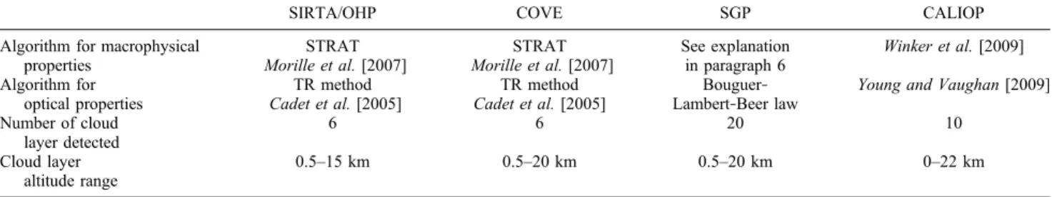
Table 2. Lidar Algorithms, Products, and Database References

SIRTA/OHP COVE SGP CALIOP

Algorithm for macrophysical properties STRAT Morille et al. [2007] STRAT Morille et al. [2007] See explanation in paragraph 6 Winker et al. [2009] Algorithm for optical properties TR method Cadet et al. [2005] TR method Cadet et al. [2005] Bouguer‐ Lambert‐Beer law

Young and Vaughan [2009] Number of cloud layer detected 6 6 20 10 Cloud layer altitude range 0.5–15 km 0.5–20 km 0.5–20 km 0–22 km

Table 3. Number of Profiles for Each Site According to CALIOP and Ground‐Based Lidara

Number of Profiles

SIRTA OHP SGP COVE

CALIOP data 14,530 14,056 14,401 14,226

Extended regional statistics 78,076 36,583 263,600 123,635

Coincident data 21,437 10,668 64,600 30,825

a_{We consider a 2 year CALIOP data set, ground}_{‐based data set for the} data coincident with CALIOP overpasses, and ground‐based data set in all over the cases.

(5)

twice per 16 day repeat cycle, providing 45 sampling opportunities per year. Extending the domain to a 2° × 6° latitude‐longitude box yields 300 (day + night) overpasses with about 45 samples each, resulting in about 14000 samples (see Table 3).

[10] The ground‐based lidars provide one sample every 5 or 10 min. For each observatory we use two different data sets: (1) a coincident data set based on the July 2006 through June 2008 period to sample the same seasons. We limit the ground‐based data to daytime and nighttime hours within ±1.5 h of the nominal satellite overpass times (i.e., about 0150 and 1350 LST) to avoid potential diurnal cycle biases; (2) an extended regional statistic is derived from multiple year data (24 to 60 months depending on the observatory), but ensuring an even sampling of seasons. Table 3 shows the number of profiles for CALIOP and ground‐based lidars for the two different data sets. The coincident data in year and time correspond to more than 10000 measurements for OHP, 21,000 for SIRTA, and 60,000 and 30,000 for SGP and COVE, respectively. These samples are collected over 314, 424, 521, and 304 days at OHP, SIRTA, SGP and COVE, respectively. Extended regional statistics contain more than three times more samples.

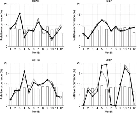
[11] CALIOP data provides a more homogeneous sam-pling through the year than any of ground‐based lidars. Figure 1 shows the sampling per month for each site obtained by CALIOP and the ground‐based lidars expressed in % of the total observations. The bars correspond to the CALIOP frequency over each site, and the lines to the ground lidar frequencies (solid line for the extended regional statistics

and dashed line for the coincident data). The monthly rela-tive occurrence ranges between 7 and 10% for CALIOP over all sites against 0 to 20% for the OHP ground‐based lidar, 3 to 16% at SIRTA, 4 to 16% at COVE and SGP. 3.2. Macrophysical Properties

3.2.1. Altitude

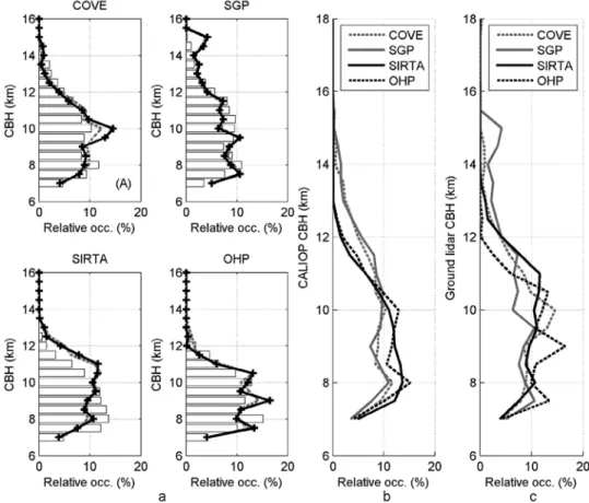
[12] Figure 2 shows the vertical distribution of CBH when clouds are present in the troposphere above 7 km (defined as the cloud base height above 7 km). CBH ranges 7–13 km over the two European sites and 7–15 km for the U.S. coastal and continental sites, as a result of a thicker summer troposphere. At SGP the distribution derived from CALIOP is multimodal with peaks at 8 and 10 km. At COVE both distributions range from 7 to 15 km. At SIRTA the dis-tributions differ in several aspects: CBH distribution from CALIOP ranges about 2 km less than that from the ground site, and peaks at 8 km, versus 8–11 km. At OHP the CALIOP and ground‐based lidar are similar, however somewhat noised for ground‐based lidar due to less frequent sampling. Clouds with CBH higher than 14 km over continental United States and CBH higher than 12 km over French sites have structures that are both geometrically and optically very thin (not shown). On Figure 2b, CBH derived from CALIOP at the four sites are superimposed, while CBH from the four ground lidars are shown on Figure 2c. For CALIOP data, all the distributions suggest several modes exhibiting two maxima centered at 8 and 10 km but the two distributions of U.S. sites extend further vertically with a maximum of cloud base altitude near 16 km (13 km over the Figure 1. Annual distribution of data sampling for CALIOP and ground‐based lidar data sets.

(6)

French sites). For ground‐based lidars, the tendencies are similar except for the important population of cirrus cloud whose altitude is higher than 11 km (27%) at SIRTA compared to 8% at OHP.

[13] Table 4 shows the CBH distribution statistics. As CBH distributions are not normal distributions, the width of the distribution is characterized by the pseudodeviation standard noted here Pstd. Dev and based on the interquartile range divided by 1.349 for scale [Lanzante, 1996]. The interquartile range is the difference of the upper quartile (quartile of order 0.75) minus the lower quartile (quartile of order 0.25). The CBH distributions at U.S. coastal and continental sites have a larger and higher mode (pseudos-tandard deviation near 2.0 km) compared to French sites (pseudostandard deviation near 1.5 km), consistent with a more pronounced range in tropospheric depth. Average CBH from CALIOP and ground data differ from +0.4 to −0.5 km, depending on location.

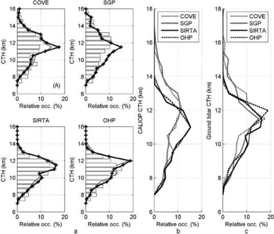
[14] Figure 3 shows the vertical distribution of the cloud top height when clouds are present in the troposphere above 7 km. The top height of cirrus clouds range 7–14 km over the French sites and 7–16 km over the U.S. sites. Over the SGP site the ground‐based Raman lidar shows a multimodal distribution peaking around 11.5 km, with a second much smaller mode around 15 km. Over the COVE site, CTH maximum occurrence is given at 12 km by CALIOP, 1 km

higher up than the micropulse ground‐based lidar. CTH distributions derived from ground‐based and spaceborne lidars over OHP and SIRTA agree also within 0.5 km. Again the CALIOP data do not contain occurrences of CTH higher than 13 km (14 km) above SIRTA (OHP). Figure 3 compares cloud top height on each site derived from CALIOP (Figure 3b) and ground‐based lidar (Figure 3c). For CALIOP data, French site distributions suggest a unique mode exhibiting one maximum centered at 11 km. The two distributions of U.S. sites have a much broader distribution with a maximum centered between 12 and 13 km with a maximum cloud top height 2 km higher than French sites. For ground‐based lidar, the distributions are similar at all sites: the highest cirrus cloud top height is almost 2 km lower for French sites compared to U.S. sites (40% of the Figure 2. (a) Vertical distributions of cloud base height CALIOP‐ground comparisons at each site.

His-tograms correspond to CALIOP data for July 2006 through June 2008 period, and black and dashed gray lines correspond to ground‐based data for extended and coincident periods (defined in Table 3), re-spectively. (b) Distributions derived from CALIOP data and (c) distributions derived from ground‐based lidar data.

Table 4. Average and Pseudostandard Deviation of Cloud Base Height Derived From Ground‐Based Lidar and CALIOPa

Sites Average (km) Pstd. Dev.(km)

COVE 9.76 (9.69) 1.83 (2.04)

SGP 9.59 (9.87) 1.76 (2.05)

SIRTA 9.65 (9.06) 1.73 (1.47)

OHP 9.15 (9.20) 1.53 (1.52)

a

CALIOP data given in parentheses. Pstd. Dev.; pseudostandard deviation.

(7)

distribution above 12 km for U.S. sites against 26% for French site).

[15] Table 5 shows the distribution statistics on cloud top height (average and pseudostandard deviation) derived from CALIOP and ground lidar for each observatory. The dis-tribution of cirrus cloud top height at U.S. coastal and continental sites have a larger and higher mode (pseudos-tandard deviation near 2.1 km for CALIOP data) compared to French sites (standard deviation near 1.5 km) noted with CALIOP and ground‐based lidar.

3.2.2. Geometrical Thickness

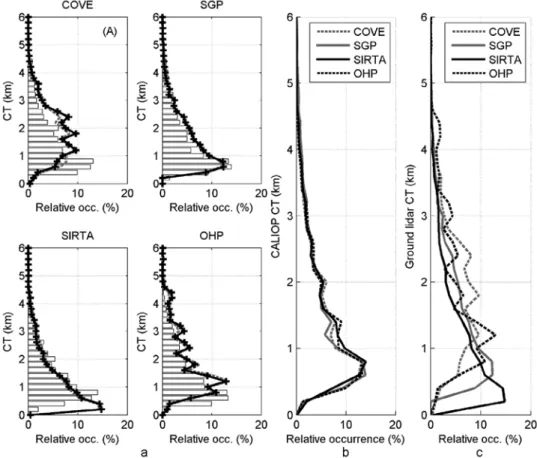
[16] Figure 4 shows the PDF of cirrus cloud geometrical thickness over each observatory derived from CALIOP and ground‐based lidars for a constant thickness step of 0.2 km. Results show that the cloud thickness derived from ground‐ based lidars (CALIOP) over French and U.S. sites range 0.5–5 km (0.5–4.5 km). For CALIOP data, distributions at all sites are nearly identical and suggest a unique mode exhibiting one maximum centered at 0.6 km with 35% of relative occurrence. On the contrary, cloud geometrical thicknesses derived from ground‐based lidars are not con-sistent from one site to another: SIRTA (SGP) site peaks at 0.5 km (0.7 km) with 15% of relative occurrence (12%), OHP peaks at 1.2 km (12%), and COVE at 1.5 km (9%). The discrepancies between ground and CALIOP data are

most important over COVE and OHP. Note that, SGP data do not provide cirrus cloud thickness less than 0.4 km. Table 6 shows the distribution statistics on cirrus cloud geometrical thickness (average and pseudostandard deviation) derived from CALIOP and ground lidar for each observatory, con-firming the discrepancies. Note that as lidar vertical resolu-tion decreases (Table 1) the cloud geometrical thickness average increases from 1.2 to 1.9 km.

3.3. Optical Thickness

[17] Figure 5 show the cumulative occurrence of cloud optical thickness in the regional data sets. The cirrus cloud optical thickness shown here corresponds to the total cloud optical thickness observed on the whole atmospheric col-Figure 3. (a) Vertical distributions of cloud top height CALIOP‐ground comparisons at each site.

His-tograms correspond to CALIOP data for July 2006 through June 2008 period, and black and dashed gray lines correspond to ground‐based data for extended and coincident periods (defined in Table 3), respectively. (b) Distributions derived from CALIOP data and (c) distributions derived from ground‐based lidar data.

Table 5. Average and Pseudostandard Deviation of Cloud Top Height Derived From Ground‐Based Lidar and CALIOPa

COVE 11.61 (11.23) 1.59 (2.12)

SGP 11.16 (11.44) 1.63 (2.06)

SIRTA 10.82 (10.54) 1.37 (1.56)

OHP 11.00 (10.63) 1.33 (1.50)

a

(8)

umn (i.e., the sum of all the cirrus cloud layers in a given profile). Figure 5c reveals that 7–25% of the cloud distri-bution falls in the subvisible category (COD < 0.03), as defined by Sassen and Benson [2001]. Between 48 and 66% falls in the semitransparent category (0.03 < COD < 0.3), while 9–42% falls in the moderate cirrus category (0.3 < COD < 3). Additionally, we find that 33–64% of the observed cirrus clouds have an optical thickness less than 0.1, which is the lower detection limit typically attributed to satellite passive sounders [Stubenrauch et al., 2006]. Significant differences appear between CALIOP and ground‐based lidars that are discussed in section 4. Cloud optical thicknesses derived from CALIOP at the four sites are consistent with each other, contrary to what is obtained from ground data. Cirrus cloud over U.S. continental and coastal sites are optically thicker with 35% of moderate cirrus cloud against 10% over French sites.

4. Discussions on Possible Sources of Bias

[18] Statistics of high‐altitude cloud macrophysical prop-erties are directly driven by lidar sampling versus life cycle of cirrus cloud and algorithms versus instrument differences. In this section, we analyze five aspects likely to induce biases in our comparisons. We distinguish on the one hand, the geophysical sources of bias and in the other hand the

instrument and algorithm differences. We analyze the in-fluence of the (1) annual and (2) diurnal variability of the macrophysical properties, (3) the impact of low‐level clouds, (4) the multiple layer detection capacity and (5) the calculation of the cloud optical thickness.

4.1. Seasonal Variations

[19] Table 7 shows the seasonal variations of cloud base height, cloud top height and cloud geometrical thickness above each site derived from CALIOP data. Above COVE and SGP, mean cloud base and top heights are about 1.5 km higher in summer than in winter. In addition, summertime PDFs of cloud base and top heights are broader than win-tertime PDFs, as evidenced by 50% greater pseudo standard Figure 4. (a) Vertical distributions of cloud geometrical thickness CALIOP‐ground comparisons at each

site. Histograms correspond to CALIOP data for July 2006 through June 2008 period, and black and dashed gray lines correspond to ground‐based data for extended and coincident periods (defined in Table 3), respectively. (b) Distributions derived from CALIOP data and (c) distributions derived from ground‐based lidar data.

Table 6. Average and Pseudostandard Deviation of Cloud Thickness Derived From Ground‐Based Lidar and CALIOPa

COVE 1.85 (1.54) 0.97 (0.92)

SGP 1,57 (1.57) 0.99 (0.93)

SIRTA 1.17 (1.47) 0.95 (0.82)

OHP 1.85 (1.43) 1.03 (0.80)

a

(9)

Figure 5. (a) Cumulative distributions (%) of cloud optical thickness CALIOP‐ground comparisons at each site. Black lines correspond to CALIOP data for July 2006 through June 2008 period, and dashed gray and dashed black lines correspond to ground‐based data for extended and coincident periods (fined in Table 3), respectively. (b) Distributions derived from CALIOP data and (c) distributions de-rived from ground‐based lidar data.

Table 7. Average Cloud Base Height, Cloud Top Height, and Cloud Thickness Separating Seasonal CALIOP Overpasses for the Four Observatoriesa

Average (km)

Winter Spring Summer Autumn All Cases

COVE CBH 9.13 9.50 10.51 9.46 9.69 CTH 10.73 10.98 12.00 11.01 11.23 CT 1.60 1.48 1.48 1.63 1.54 SGP CBH 9.19 9.37 10.85 9.63 9.87 CTH 10.83 10.96 12.45 11.04 11.44 CT 1.65 1.59 1.60 1.41 1.57 SIRTA CBH 9.25 8.79 9.12 9.08 9.06 CTH 10.74 10.23 10.54 10.60 10.54 CT 1.49 1.46 1.42 1.52 1.47 OHP CBH 9.10 8.74 9.39 9.58 9.20 CTH 10.46 10.23 10.64 11.11 10.63 CT 1.36 1.49 1.25 1.53 1.43 a

CBH, cloud base height; CTH, cloud top height; CT, cloud thickness.

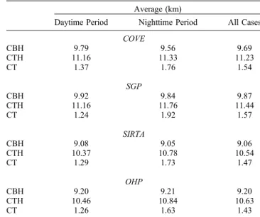
Table 8. Average Cloud Base Height, Cloud Top Height, and Cloud Thickness Separating Daytime and Nighttime CALIOP Overpasses for the Four Observatoriesa

Average (km)

Daytime Period Nighttime Period All Cases

COVE CBH 9.79 9.56 9.69 CTH 11.16 11.33 11.23 CT 1.37 1.76 1.54 SGP CBH 9.92 9.84 9.87 CTH 11.16 11.76 11.44 CT 1.24 1.92 1.57 SIRTA CBH 9.08 9.05 9.06 CTH 10.37 10.78 10.54 CT 1.29 1.73 1.47 OHP CBH 9.20 9.21 9.20 CTH 10.46 10.84 10.63 CT 1.26 1.63 1.43 a

CBH, cloud base height; CTH, cloud top height; CT, cloud thickness.

(10)

deviations (not shown). Cloud geometrical thickness dis-tributions, however, do not reveal seasonal dependences. At OHP and SIRTA, the seasonal range of average cloud base and top heights, shown in Table 7, is less than 0.5 km, which is considerably less than and not phased with the 1.6 km winter‐summer vertical range of tropopause height observed at SIRTA [Noël and Haeffelin, 2007]. The sea-sonal dependence of cirrus cloud altitudes over U.S. conti-nental and coastal sites could be due to the deepening of the moist layer during summer as a result of vertical convective fluxes induced by solar heating of the surface. This phe-nomenon may not appear over French sites (44°N–49°N) because the boundary layer dynamics is not important enough to affect the formation of cloud higher than 7 km. Moreover, the cirrus cloud formation processes are not similar over central and eastern U.S. (synoptic weather systems, i.e., fronts in fall and winter months and convection in the summer months) and French (essentially fronts in all the seasons) sites.

[20] The seasonal cycle of cirrus cloud altitude combined with nonhomogeneous ground‐based lidar samplings could induce discrepancies between CALIOP and ground‐based lidar in cloud base and top height distributions. Data sam-pling at COVE is biased low in winter (15%) and high in summer (35%), as shown in Figure 1. The convolution of sampling and seasonal cycle in cirrus cloud altitude results in a positive 0.1 km bias in mean cloud base and top altitude in the ground‐based data. The homogeneous sampling at SGP does not introduce bias in comparisons at that site in spite of strong seasonal variations. At SIRTA and OHP,

because of quasi absence of seasonal cycle in cirrus altitude, the impact of irregular seasonal sampling is estimated to have little or no effect on mean cloud base and top altitudes. 4.2. Diurnal Cycle

[21] Table 8 shows the average cloud base and top alti-tudes and the average geometrical thickness for each site separating CALIOP daytime and nighttime overpasses. The average cloud base height is found to be nearly identical above all but one site (COVE) where average daytime CBH is 0.2 km higher than that of nighttime. The average cloud top altitude is 0.1–0.5 km higher at night than during the day (0.1 km at COVE, 0.5 km at SGP, 0.4 at SIRTA and 0.3 at OHP). The average geometrical thickness is thus found to be 0.3–0.5 km thicker at night than during the day. In addition, we find that the occurrence of optically very thin clouds (optical thickness < 0.03) in CALIOP data is 10–25% more frequent at night than during the day (not shown). Better signal‐to‐noise ratio at night allows optically thinner cloud to be detected. The greater cloud geometrical thickness de-rived at night can thus be due to a better detection of the base and the top of the cirrus clouds (low scattering ratio) resulting in thicker clouds.

[22] Ground‐based data day‐night sampling at COVE and SGP is homogeneous. For SIRTA (OHP), only daytime (nighttime) CALIOP data are considered to be consistent with ground‐based sampling. Only ground‐based data within ±1.5 h of the satellite local overpass times are used in the statistics. However, the micropulse lidar at COVE is less sensitive to high‐altitude clouds during daytime because of Figure 6. Vertical distribution of the cloud base height (CBH), cloud top height (CTH), and cloud

thick-ness (CT) over SGP site, distinguishing cirrus cloud situations with (black dashed line) and without low‐ level clouds below (i.e., CBH < 7 km, black solid line) based on CALIOP data.

(11)

low daytime signal‐to‐noise ratio due to significant solar contamination. Hence the ground‐based COVE data set is biased toward nighttime, which could explain 0.2 km dis-crepancy in cloud geometrical thickness between ground and CALIOP data.

4.3. Effect of Low‐Level Clouds

[23] Next we study possible effects of presence or absence of low‐altitude clouds (a cloud layer between ground and 7 km) on the cirrus cloud statistics and comparisons (Figure 6). Table 9 shows the mean base and top altitude and the mean geometrical thickness above each site derived from CALIOP overpasses when low‐altitude clouds are (with) and are not (without) present. Cirrus clouds are 0.1– 0.3 km thicker, geometrically, in the absence of low‐level clouds. Cirrus cloud average base (top) altitudes are 0.1– 0.4 km (0.3–0.6 km) higher in the absence of low‐level clouds. Above SGP and COVE, we find that in summer (winter) the average geometrical thickness of cirrus clouds is greater by 0.5 km (0.1 km) when low‐level clouds are absent compared to when they are present (not shown). This difference during summer and winter period argues that dynamic feedbacks are likely to impact cirrus properties (thickness, altitude): low‐level clouds are able to decrease deep convection responsible for vertical humidity trans-port. No seasonal dependence is observed above SIRTA and OHP.

[24] Figure 7 shows the relative occurrence of clear sky (without any clouds), cirrus cloud without clouds below and cirrus cloud with clouds below, derived from CALIOP data. Occurrence of cirrus clouds is remarkably high, ranging from 33 to 43% above SIRTA and SGP, respectively. At SIRTA, cirrus clouds with low‐level clouds below are twice as frequently as cirrus clouds without low‐level clouds below, whereas for the three others sites, the rela-tive occurrence of with/without low‐level clouds below is

Figure 7. Relative occurrence of clear sky (without any clouds, white area), cirrus clouds without clouds below (gray area), and cirrus cloud with clouds below (black area), derived from CALIOP data.

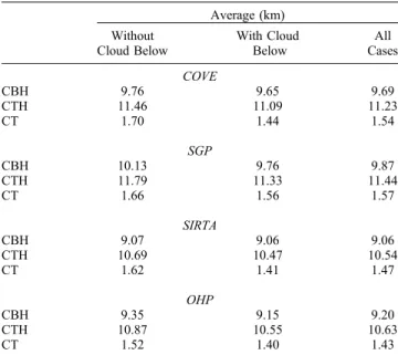
Table 9. Average Cloud Base Height, Cloud Top Height, and Cloud Thickness Separating CALIOP Overpasses With and Without Cloud Below 7 km Height for the Four Observatoriesa

Average (km) Without Cloud Below With Cloud Below All Cases COVE CBH 9.76 9.65 9.69 CTH 11.46 11.09 11.23 CT 1.70 1.44 1.54 SGP CBH 10.13 9.76 9.87 CTH 11.79 11.33 11.44 CT 1.66 1.56 1.57 SIRTA CBH 9.07 9.06 9.06 CTH 10.69 10.47 10.54 CT 1.62 1.41 1.47 OHP CBH 9.35 9.15 9.20 CTH 10.87 10.55 10.63 CT 1.52 1.40 1.43

a_{CBH, cloud base height; CTH, cloud top height; CT, cloud thickness.}

(12)

50%. Overcast low‐level clouds are likely to prevent ground‐based lidars from detecting high‐altitude clouds. These situations correspond to about 50% (black to [black +gray] histogram ratio) of cirrus cloud occurrences at SGP, COVE and OHP and about 70% at SIRTA. Hence, altitude and geometrical thickness distribution differences (Figures 2, 3 and 4) between CALIOP and ground‐based lidar can be partially explained by the difference in sampling without low‐level clouds below (ground‐based data) versus all the time (CALIOP data). This sampling difference can explain 0.05–0.2 km, 0.15–0.3, and 0.05–0.15 km dis-crepancies in cloud base height, top height and geometrical thickness, respectively.

4.4. Effect of Multiple Layers

[25] Figure 8 shows the occurrence of single and multiple cirrus cloud layers for each site derived from ground‐based lidars and CALIOP. Over all sites, CALIOP data reveal a single cirrus cloud layer in 80% of cloudy situations, a second cirrus cloud layer in 16% of the cases a third cirrus cloud layer in 3% of the cases, and more than 3 cirrus cloud layers 1% of the cases. Ground‐based data exhibit large differences between sites: SIRTA data show 30% multiple layer cirrus clouds; SGP data show 15% multiple layer cirrus clouds, whereas COVE/OHP data reveal about 11% multiple cirrus cloud layers. This low percentage is related to the vertical resolution of the lidars operated at each site: 75 m (COVE and OHP) against 15 m for SIRTA and 30 m or 60 m for CALIOP below and above 8 km, respectively. Cloud detection algorithms (e.g., STRAT by Morille et al. [2007]) require a minimum of few consecutive cloud pixels in the backscattered lidar profile to detect and classify a

cloudy or a clear atmosphere. Hence, cirrus clouds are sta-tistically thicker for low lidar vertical resolution (COVE/ OHP) than for SIRTA and CALIOP (see Figure 4). Lidars characterized by a low vertical resolution are likely to group cirrus clouds separated by thicker clear atmosphere than for those with a high vertical resolution. Cirrus clouds geo-metrical thickness over SIRTA (SGP) derived from ground‐ based lidar peaks to 200 m (400 m) against 600 m for CALIOP which confirms the relationship between vertical resolution, lidar algorithm and cirrus cloud geometrical thickness.

[26] Table 10 shows the average cloud base height, cloud top height and cloud thickness separating single layer situa-tions (representing about 80% of situasitua-tions), double layer situations (about 16% of situations) and triple and quadruple layer situations (representing about 3 and 1% of situations). Note that in a double layer situation, the average CBH (or CTH or CT) value is derived by averaging the CBH (or CTH or CT) of the two layers. Table 10 shows that in double layer situations, the average CBH (CTH) is lower by 0.4 to 0.8 km (0.7 km) than in single layer situations. Because situations with 3 or more layers occur very infrequently, the mean CBH and CTH cannot be compared to single layer mean CBH and CTH in a significant manner. In multilayer situations, we find that the mean cloud layer thickness (CT) is significantly reduced compared to single layer situations (10% reduction for double layer situations and 25% reduction for triple layer situations). Considering jointly the results of Figure 8 and Table 10, we evaluate that the discrepancies in lidar vertical resolution will result in 0.0 km, 0.1 km and 0.1 km inconsistencies in average cloud base height, cloud Figure 8. Number of cirrus cloud layers (one, two, three, four, and five cloud layers) at each site

(13)

top height and cloud geometrical thickness comparisons, respectively.

[27] In this study we consider (1) all the CALIOP and ground‐based lidar profiles for the altitude and geometrical

thickness retrievals and (2) only the profiles with an above molecular signal (for ground‐based lidar). The retrieved Cloud Top Height (CTH) is an “apparent CTH,” which might be lower than the“true CTH.” For the ground‐based lidar data set, the opaque cirrus clouds represent for example 35% for COVE site and concerning the CALIOP data set, only 7%. Hence, the opaque cloud population represents a significant fraction for the ground‐based data set. To quantify the impact of the difference between the “true CTH” (when COT is calculated) and the “apparent CTH” (for all the data set with and without COT retrieval), we compare the PDF distribution of the CTH for all the cloud profiles and only for those with cloud optical thickness retrieval. We have a difference of 25, 65 and 54 m between the average“true CTH” and the average “apparent CTH” for COVE, SIRTA and OHP site, respectively. It also implies that there are few clouds in this data set with optical thickness on the order of 3 or larger. All the statistics for CALIOP data are the same for the“true” and the “apparent” CTH (only 7% of the cirrus cloud profiles not provide COT retrieval). This implies that the criteria for classifying a CTH as “apparent” are too strict and the ground‐based instru-ments actually find the“true CTH” very often.

4.5. Impact of Cloud Optical Thickness Retrieval Algorithms

[28] Figure 9 shows cirrus cloud optical thickness dis-tributions derived from ground‐based lidars (transmission method: TR method) and CALIOP (transmission method:

Table 10. Average of Cloud Base Height, Cloud Top Height, and Cloud Thickness Separating the Different Cirrus Cloud Layers for Each CALIOP Overpass Over the Four Observatoriesa

Average (km) One Cloud Layer Two Cloud Layers Three Cloud Layers Four

Cloud Layers All COVE CBH 9.84 9.42 9.48 9.05 9.69 CTH 11.53 10.89 10.81 10.18 11.23 CT 1.69 1.47 1.33 1.13 1.54 SGP CBH 10.20 9.41 9.55 9.98 9.87 CTH 11.85 11.07 10.91 11.11 11.44 CT 1.65 1.66 1.36 1.13 1.57 SIRTA CBH 9.17 8.72 8.99 9.00 9.06 CTH 10.79 10.18 10.13 10.01 10.54 CT 1.62 1.46 1.14 1.01 1.47 OHP CBH 9.34 8.92 8.83 8.63 9.20 CTH 10.87 10.32 10.02 9.79 10.63 CT 1.53 1.40 1.19 1.16 1.43

a_{CBH, cloud base height; CTH, cloud top height; CT, cloud thickness.}

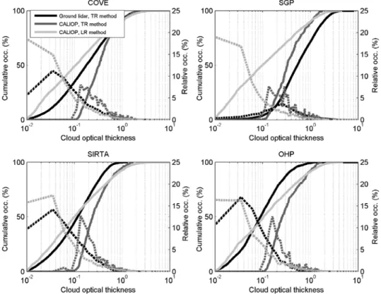
Figure 9. Cumulative and relative distributions of cirrus cloud optical thickness derived from ground‐ based lidar and CALIOP data at each site. The continuous line corresponds to cumulative occurrence and the dashed line to relative occurrence. The black line corresponds to ground‐based lidar cloud optical thickness (COT), and the gray lines correspond to CALIOP COT. Abbreviations: TR method, transmis-sion method; LR method, lidar ratio method.

(14)

TR method and lidar ratio method: LR method) over U.S. and French sites. The TR method is applied to CALIOP data for clouds ranging about 0.1–3 in optical thickness. Because the TR method requires high signal‐to‐noise ratio in the molecular region above and below the cloud layer, it can only applied to about 10% of CALIOP data. The TR method is applied to ground‐based lidar data for clouds ranging about 0.001–3 in optical thickness. It is successfully applied to about 50% of ground‐based lidar profiles. The LR method is applied to about 95% of CALIOP profiles where cirrus layers are identified. Note that the LR method is not applied to the ground‐based lidar data sets. Relative oc-currences are derived using a constant cloud optical thick-ness interval of 0.025 and displayed with logarithm scale for x axis. Significant discrepancies appear for subvisible cirrus cloud (i.e., 0.01 < COT < 0.03). CALIOP LR data reveal that subvisible clouds represent about 25% of the distribu-tion, while 20% is found in SIRTA and OHP data, but only 10% and 5% in COVE and SGP data, respectively. The semitransparent class (0.03 < COT < 0.3) is found to rep-resent 50% of the distribution in the CALIOP LR data, about 60% of the distribution in both SIRTA and OHP data, and about 50% in both COVE and SGP data. The thickest class (0.3 < COT < 3) represents about 25% of the distri-bution in CALIOP LR data, 20% in SIRTA and OHP data and more than 40% of COVE and SGP data.

[29] To study the distribution in CALIOP TR data, we focus on the 0.1–3 COT range, as shown in Figure 10. We find that the semitransparent population represents 50% of the 0.1–3.0 distribution in CALIOP TR data above the

COVE and SGP sites, which is consistent with COVE and SGP ground data. Above SIRTA and OHP, the semitrans-parent population represents 60% of the distribution of CALIOP TR data, also consistent with SIRTA data. This population is found to represent 70% of the OHP data. We also note a better agreement between CALIOP TR and LR data above the two U.S. sites than above the French sites.

5. Conclusion

[30] Ground‐based lidar and CALIOP data sets gathered over four midlatitude sites, two U.S. and two French sites, are used to evaluate the consistency of cloud macro-physical and optical property climatologies that can be derived by such data sets. The data sets cover 2 years of quasi‐simultaneous measurements by the spaceborne instru-ment CALIOP and four ground‐based lidars. Cloud base height, cloud top height, cloud geometrical thickness and cloud optical thickness of high‐altitude clouds distributions are analyzed.

[31] We note that the consistency in average cloud height (both base and top height) between the CALIOP and ground data sets ranges from−0.4 km to +0.5 km. The consistency in pseudostandard deviations of the cloud height distribu-tions between the two data sets range 0–0.5 km. We find that cloud geometrical thickness distributions vary signifi-cantly between the different data sets, due in part to the original vertical resolutions of the lidar profiles. Average cloud geometrical thicknesses vary from 1.2 to 1.9 km, i.e., by more than 50%. Cloud optical thickness distributions in Figure 10. Cumulative and relative occurrence of cirrus cloud optical thickness greater than 0.1 derived

from CALIOP (TR and LR method) and ground‐based lidar data. The continuous line corresponds to cumulative occurrence and the dashed line to relative occurrence. The black line corresponds to ground‐ based lidar COT, and the gray lines correspond to CALIOP COT.

(15)

subvisible, semitransparent and moderate intervals differ by more than 50% between ground‐ and space‐based data sets. However, all lidar data sets agree that the fraction of cirrus clouds with optical thickness below 0.1 (not included in historical cloud climatologies) represent 30–50% of the nonopaque cirrus class. So while the radiative effects of a 0.1 optical thickness cloud maybe considered tenuous, the cumulative effect on the radiative balance due to the high abundance is likely to be significant [McFarquhar et al., 2000].

[32] Discrepancies between the ground and CALIOP data sets are attributed in part to sampling. Our study shows that differences in average cloud base altitude (cloud top alti-tude) between ground and CALIOP data sets can be attributed (1) to irregular sampling of seasonal variations in the ground‐ based data (0.0–0.1 km (0.0–0.1 km)), (2) to day‐night dif-ferences in detection capabilities by CALIOP (0.0–0.2 km (0.0–0.2 km)) and (3) to the restriction to situations without low‐level clouds in ground‐based data (0.0–0.2 km (0.1– 0.3 km)). Finally, cloud geometrical thicknesses are not affected by irregular sampling of seasonal variations in the ground‐based data, while up to 0.0–0.2 km and 0.1–0.3 km differences can be attributed to day‐night differences in detection capabilities by CALIOP and to the restriction to situations without low‐level clouds in ground‐based data, respectively. We find that the lidar vertical resolution can have an effect on the number of single versus multiple layer situations detected. This effect does not affect the average cloud base height, but may affect both cloud top height and cloud geometrical thickness by 0.1 km.

[33] For high‐altitude clouds, using consistent transmis-sion‐based retrieval methods, COT distributions from ground and CALIOP data are found to be consistent within about 10%. This comparison is limited to COT greater than 0.1 and to about 10% of the CALIOP retrievals. We find that the CALIOP LR data is biased toward lower optical depth when compared to the ground‐based data sets. These comparisons reveal the high sensitivity to the retrieval al-gorithm. Hence this exercise will have to be conducted again for the next release of CALIOP data. Overall, the results show that cirrus clouds with COD < 0.1 and COD < 0.3 (detection limits for infrared sounders and visible im-agers) represent 25–50% and 50–75% of the nonopaque cirrus class. The occurrence of cirrus clouds at the global scale is thus likely to be significantly underestimated in historical cloud climatologies.

[34] Acknowledgments. The authors would like to thank the Centre National d’Etudes Spatiales (CNES), the Centre National de la Recherche Scientifique (CNRS), the Office National d’Etude et de Recherche Aéro-spatiale (ONERA), and the Climate Change Research Division of the U.S. Department of Energy as part of the Atmospheric Radiation Measure-ment (ARM) Program for their support in this study. The data at the COVE site are funded by the NASA Earth Observing System project. We extend our acknowledgments to the technical and computer staff of each observa-tory for taking the observations and making the data set easily accessible and to the ICARE datacenter for providing CALIOP level‐2 data. The authors are grateful to the anonymous reviewers for their useful comments.

References

Ackerman, S. A., R. E. Holz, R. Frey, E. W. Eloranta, B. Maddux, and M. McGill (2008), Cloud detection with MODIS: Part II validation, J. Atmos. Oceanic Technol., 25, 1073–1086, doi:10.1175/2007JTECHA1053.1.

Ackerman, T. P., and G. M. Stokes (2003), The Atmospheric Radiation Measurement Program, Phys. Today, 56, 38–44, doi:10.1063/1.1554135. Barnes, W. L., T. S. Pagano, and V. V. Salomonson (1998), Prelaunch characteristics of the Moderate Resolution Imaging Spectroradiometer (MODIS) on EOS‐AM1, IEEE Trans. Geosci. Remote Sens., 36(4), 1088–1100, doi:10.1109/36.700993.

Cadet, B., V. Giraud, M. Haeffelin, P. Keckhut, A. Rechou, and S. Baldy (2005), Improved retrievals of cirrus cloud optical properties using a combination of lidar methods, Appl. Opt., 44, 1726–1734, doi:10.1364/ AO.44.001726.

Chen, T., W. B. Rossow, and Y. Zhang (2000), Radiative effects of cloud‐ type variations, J. Clim., 13, 264–286, doi:10.1175/1520-0442(2000) 013<0264:REOCTV>2.0.CO;2.

Chen, W. N., C. W. Chiang, and J. B. Nee (2002), Lidar ratio and depolar-isation ratio for cirrus clouds, Appl. Opt., 41, 6470–6476, doi:10.1364/ AO.41.006470.

Comstock, J. M., T. P. Ackerman, and G. G. Mace (2002), Ground‐based lidar and radar remote sensing of tropical cirrus clouds at Nauru Island: Cloud statistics and radiative impacts, J. Geophys. Res., 107(D23), 4714, doi:10.1029/2002JD002203.

Currey, J. C., et al. (2007), Cloud‐aerosol lidar infrared Pathfinder satellite observations, data management system: Data products catalog, Doc. PC‐ SCI‐503, 97 pp., NASA Langley Res. Cent., Hampton, Va.

Dupont, J.‐C., and M. Haeffelin (2008), Observed instantaneous cirrus radiative effect on surface‐level shortwave and longwave irradiances, J. Geophys. Res., 113, D21202, doi:10.1029/2008JD009838. Fernald, F. G., B. J. Herman, and J. A. Reagan (1972), Determination of

aerosol height distributions by lidar, J. Appl. Meteorol., 11, 482–489, doi:10.1175/1520-0450(1972)011<0482:DOAHDB>2.0.CO;2. Goldfarb, L., P. Keckhut, M. L. Chanin, and A. Hauchecorne (2001),

Cir-rus climatological results from lidar measurement at OHP (44°N, 6°E), Geophys. Res. Lett., 28, 1687–1690, doi:10.1029/2000GL012701. Goldsmith, J. E. M., F. H. Blair, S. E. Bisson, and D. D. Turner (1998),

Turn‐key Raman lidar for profiling atmospheric water vapor, clouds, and aerosols, Appl. Opt., 37, 4979–4990, doi:10.1364/AO.37.004979. Haeffelin, M., et al. (2005), SIRTA, a ground‐based atmospheric

observa-tory for cloud and aerosol research, Ann. Geophys., 23, 262–275. Keckhut, P., F. Borchi, S. Bekki, A. Huachecorne, and M. SiLiaouina

(2006), Cirrus classification at midlatitude from systematic lidar observa-tions, J. Appl. Meteorol. Climatol., 45, 249–258.

Lanzante, J. R. (1996), Resistant, robust and nonparametric techniques for the analysis of climate data: Theory and examples, including applications to historical radiosonde station data, Int. J. Climatol., 16, 1197–1226, doi:10.1002/(SICI)1097-0088(199611)16:11<1197::AID-JOC89>3.0. CO;2-L.

McFarquhar, G. M., A. J. Heymsfield, J. Spinhirne, and B. Hart (2000), Thin and subvisual tropopause tropical cirrus: Observations and radiative impacts, J. Atmos. Sci., 57, 1841–1853.

Morille, Y., M. Haeffelin, P. Drobinski, and J. Pelon (2007), STRAT: An automated algorithm to retrieve the vertical structure of the atmosphere from single‐channel lidar data, J. Atmos. Oceanic Technol., 24, 761– 775, doi:10.1175/JTECH2008.1.

Nazaryan, H., M. P. McCormick, and W. P. Menzel (2008), Global char-acterization of cirrus clouds using CALIPSO data, J. Geophys. Res., 113, D16211, doi:10.1029/2007JD009481.

Noël, V., and M. Haeffelin (2007), Midlatitude cirrus clouds and multiple tropopauses from a 2002–2006 climatology over the SIRTA observatory, J. Geophys. Res., 112, D13206, doi:10.1029/2006JD007753.

Plana‐Fattori, A., et al. (2008), High clouds characteristics from multi‐year ground based lidar observation in France, J. Appl. Meteorol. Climatol., 48, 1142–1160, doi:10.1175/2009JAMC1964.1

Platnick, S., M. D. King, S. A. Ackerman, W. P. Menzel, B. A. Baum, J. C. Riédi, and R. A. Frey (2003), The MODIS cloud products: Algorithms and examples from Terra, IEEE Trans. Geosci. Remote Sens., 41, 459– 473, doi:10.1109/TGRS.2002.808301.

Platt, C. M. R. (1973), Lidar and radiometric observations of cirrus clouds, J. Atmos. Sci., 30, 1191–1204, doi:10.1175/1520-0469(1973)030<1191: LAROOC>2.0.CO;2.

Rossow, W. B., and R. A. Schiffer (1999), Advances in understanding clouds from ISCCP, Bull. Am. Meteorol. Soc., 80, 2261–2286, doi:10.1175/1520–0477.

Rutledge, C. K., G. L. Schuster, T. P. Charlock, F. M. Denn, W. L. Smith Jr., B. E. Fabbri, J. J. Madigan Jr., and R. J. Knapp (2006), Offshore radiation observations for climate research at the CERES ocean validation experi-ment, Bull. Am. Meteorol. Soc., 87, 1211–1222, doi:10.1175/BAMS-87-9-1211.

Sassen, K., and S. Benson (2001), A midlatitude cirrus cloud climatology from the Facility for Atmospheric Remote Sensing. II. Microphysical

(16)

properties derived from lidar depolarization, J. Atmos. Sci., 58, 2103– 2112, doi:10.1175/1520-0469(2001)058<2103:AMCCCF>2.0.CO;2. Sassen, K., and J. R. Campbell (2001), A midlatitude cirrus cloud

clima-tology from the Facility for Atmospheric Remote Sensing: I. Macrophy-sical and synoptic properties, J. Atmos. Sci., 58, 481–496, doi:10.1175/ 1520-0469(2001)058<0481:AMCCCF>2.0.CO;2.

Sassen, K., and J. Comstock (2001), A midlatitude cirrus cloud climatology from the Facility for Atmospheric Remote Sensing. III. Radiative proper-ties, J. Atmos. Sci., 58, 2113–2127, doi:10.1175/1520-0469(2001) 058<2113:AMCCCF>2.0.CO;2.

Sassen, K., Z. Wang, and D. Liu (2008), The global distribution of cirrus clouds from CloudSat/CALIPSO Measurements, J. Geophys. Res., 113, D00A12, doi:10.1029/2008JD009972.

Stephens, G. L., S. C. Tsay, P. W. Stackhouse, and P. J. Flatau (1990), The relevance of the microphysical and radiative properties of cirrus clouds to climate and climatic feedbacks, J. Atmos. Sci., 47, 1742–1753, doi:10.1175/1520-0469(1990)047<1742:TROTMA>2.0.CO;2. Stubenrauch, C. J., W. B. Rossow, N. A. Scott, and A. Chédin (1999), Clouds

as seen by infrared sounders (3i) and imagers (ISCCP). Part III: Spatial heterogeneity and radiative effects, J. Clim., 12, 3419–3442, doi:10.1175/1520-0442(1999)012<3419:CASBSS>2.0.CO;2.

Stubenrauch, C. J., F. Eddounia, and L. Sauvage (2005), Cloud heights from TOVS Path‐B: Evaluation using LITE observations and distribu-tions of highest cloud layers, J. Geophys. Res., 110, D19203, doi:10.1029/2004JD005447.

Stubenrauch, C. J., A. Chedin, G. Rädel, N. A. Scott, and S. Serrar (2006), Cloud properties and their seasonal and diurnal variability from TOVS Path‐B, J. Clim., 19, 5531–5553, doi:10.1175/JCLI3929.1.

Stubenrauch, C. J., S. Cros, N. Lamquin, R. Armante, A. Chédin, C. Crevoisier, and N. A. Scott (2008), Cloud properties from Atmospheric Infrared Sounder and evaluation with Cloud‐Aerosol Lidar and Infrared Pathfinder Satellite Observations, J. Geophys. Res., 113, D00A10, doi:10.1029/2008JD009928.

Wang, P. H., P. Minnis, M. P. McCormic, G. S. Kent, and K. M. Skeens (1996), A 6‐year climatology of cloud occurrence frequency from Strato-spheric Aerosol and Gas Experiment II observations (1985–1990), J. Geophys. Res., 101, 407–429.

Webster, P. J. (1994), The role of hydrological processes in ocean‐ atmosphere interactions, Rev. Geophys., 32(4), 426–476, doi:10.1029/ 94RG01873.

Winker, D. (2003), Accounting for multiple scattering in retrievals from space lidar, Proc. SPIE Int. Soc. Opt. Eng., 5059, 128–139.

Winker, D. M., M. A. Vaughan, A. H. Omar, Y. Hu, K. A. Powell, Z. Liu, W. H. Hunt, and S. A. Young (2009), Overview of the CALIPSO mission and CALIOP data processing algorithms, J. Atmos. Oceanic Technol., 26, 2310–2323, doi:10.1175/2009JTECHA1281.1.

Wylie, D., P. Piironen, W. Wolf, and E. Eloranta (1995), Understanding satellite cirrus cloud climatologies with calibrated lidar optical depths, J. Atmos. Sci., 52, 4327–4343, doi:10.1175/1520-0469(1995) 052<4327:USCCCW>2.0.CO;2.

Young, S. A., and M. A. Vaughan (2009), The retrieval of profiles of par-ticulate extinction from Cloud Aerosol Lidar Infrared Pathfinder Satellite Observations (CALIPSO) data: Algorithm description, J. Atmos. Oceanic Technol., 26, 1105–1119, doi:10.1175/2008JTECHA1221.1.

P. Chervet and A. Roblin, ONERA, Chemin de la Hunière, F‐91751 Palaiseau CEDEX, France.

J. Comstock, PNNL, PO Box 999, MSIN: K9‐24, Richland WA 99352, USA.

J.‐C. Dupont, M. Haeffelin, Y. Morille, and V. Noël, LMD, IPSL, Ecole Polytechnique, F‐91128 Palaiseau CEDEX, France. (dupont@lmd. polytechnique.fr)

P. Keckhut, SA, IPSL, Université Versailles Saint‐Quentin, 5‐7 Boulevard d’Alembert, F‐78280 Guyancourt CEDEX, France.

D. Winker, NASA Langley Research Center, Hampton, VA 23681‐0001, USA.