Tropospheric aerosol microphysics simulation with assimilated meteorology: model description and intermodel comparison

(1)

HAL Id: hal-00303126

https://hal.archives-ouvertes.fr/hal-00303126

Submitted on 10 Oct 2007

HAL is a multi-disciplinary open access

archive for the deposit and dissemination of sci-entific research documents, whether they are pub-lished or not. The documents may come from teaching and research institutions in France or abroad, or from public or private research centers.

L’archive ouverte pluridisciplinaire HAL, est destinée au dépôt et à la diffusion de documents scientifiques de niveau recherche, publiés ou non, émanant des établissements d’enseignement et de recherche français ou étrangers, des laboratoires publics ou privés.

Tropospheric aerosol microphysics simulation with

assimilated meteorology: model description and

intermodel comparison

W. Trivitayanurak, P. J. Adams, D. V. Spracklen, K. S. Carslaw

To cite this version:

W. Trivitayanurak, P. J. Adams, D. V. Spracklen, K. S. Carslaw. Tropospheric aerosol microphysics simulation with assimilated meteorology: model description and intermodel comparison. Atmospheric Chemistry and Physics Discussions, European Geosciences Union, 2007, 7 (5), pp.14369-14411. �hal-00303126�

(2)

ACPD

7, 14369–14411, 2007 Aerosol microphysics simulation and intercomparison W. Trivitayanurak et al. Title Page Abstract Introduction Conclusions References Tables Figures ◭ ◮ ◭ ◮ Back Close

Full Screen / Esc

Printer-friendly Version Interactive Discussion

Atmos. Chem. Phys. Discuss., 7, 14369–14411, 2007 www.atmos-chem-phys-discuss.net/7/14369/2007/ © Author(s) 2007. This work is licensed

under a Creative Commons License.

Atmospheric Chemistry and Physics Discussions

Tropospheric aerosol microphysics

simulation with assimilated meteorology:

model description and intermodel

comparison

W. Trivitayanurak1, P. J. Adams1,2, D. V. Spracklen3,*, and K. S. Carslaw4

1

Department of Civil and Environmental Engineering, Carnegie Mellon University, Pittsburgh, Pennsylvania, USA

2

Department of Engineering and Public Policy, Carnegie Mellon University, Pittsburgh, Pennsylvania, USA

3

School of Engineering and Applied Sciences, Harvard University, Cambridge, Massachusetts, USA

4

Institute of Atmospheric Science, School of Earth and Environment, University of Leeds, UK

*

now at: Institute of Atmospheric Science, School of Earth and Environment, University of Leeds, UK

Received: 31 August 2007 – Accepted: 2 October 2007 – Published: 10 October 2007 Correspondence to: W. Trivitayanurak (win@cmu.edu)

(3)

ACPD

Full Screen / Esc

Abstract

We implement the TwO-Moment Aerosol Sectional (TOMAS) microphysics module into GEOS-CHEM, a CTM driven by assimilated meteorology. TOMAS has 30 size sections covering 0.01–10 µm diameter with conservation equations for both aerosol mass and number. The implementation enables GEOS-CHEM to simulate aerosol microphysics,

5

size distributions, mass and number concentrations. The model system is developed for sulfate and sea-salt aerosols, a year-long simulation has been performed, and re-sults are compared to observations. Additionally model intercomparison was carried out involving global models with sectional microphysics: GISS GCM-II’ and GLOMAP. Comparison with marine boundary layer observations of CN and CCN(0.2%) shows

10

that all models perform well with average errors of 30–50%. However, all models underpredict CN by up to 42% between 15◦S and 45◦S while overpredicting CN up to 52% between 45◦N and 60◦N, which could be due to the sea-salt emission pa-rameterization and the assumed size distribution of primary sulfate emission, in each case respectively. Model intercomparison at the surface shows that GISS GCM-II’

15

and GLOMAP, each compared against GEOS-CHEM, both predict 40% higher CN and predict 20% and 30% higher CCN(0.2%) on average, respectively. Major discrepan-cies are due to different emission inventories and transport. Budget comparison shows GEOS-CHEM predicts the lowest global CCN(0.2%) due to microphysical growth being a factor of 2 lower than other models because of lower SO₂availability. These findings

20

stress the need for accurate meteorological inputs and updated emission inventories when evaluating global aerosol microphysics models.

1 Introduction

Atmospheric aerosols impact climate in two ways: directly reflecting solar radiation, known as the aerosol direct effect (Charlson et al., 1992), and acting as cloud

con-25

densation and ice nuclei (CCN and IN, respectively), thereby changing the reflectivity 14370

(4)

ACPD

Full Screen / Esc

and the likelihood of precipitation, which is called the aerosol indirect effect (Albrecht, 1989; Twomey, 1974, 1977). The aerosol direct effect has been estimated with more certainty than the indirect effect. According to the Fourth Assessment Report of the Intergovernmental Panel on Climate Change (IPCC), the global and annual average indirect aerosol radiative forcing uncertainty range is between −1.8 and −0.3 W m−2

5

(IPCC, 2007). Note that this uncertainty range refers to only the cloud brightness ef-fect (first aerosol indirect efef-fect), not including changes in cloud lifetime and distribution (second aerosol indirect effect); this underlines the need to improve the estimate of aerosol indirect radiative forcing.

The aerosol indirect effect is caused by CCN, the subset of airborne particles that

10

become cloud droplets. To reduce uncertainty in estimates of indirect radiative forcing, the links between emissions, CCN, and cloud droplet number concentrations (CDNC) must be well simulated in models. Early attempts to predict CDNC used empirical relationships between sulfate mass and CDNC without explicitly simulating aerosol and cloud microphysics (Boucher and Lohmann, 1995; Jones et al., 1994; Martin et

15

al., 1994). This kind of empirical relationship is of limited use for locations and times other than where the relationship was measured. As pointed out by Kiehl (2000), lim-itations and uncertainties associated with the empirical approach suggest the need to take a mechanistic approach, for example by explicitly simulating aerosol number concentrations and size distributions. More recent aerosol models use a mechanistic

20

approach to predicting CCN concentrations by including size-resolved aerosol micro-physics Adams and Seinfeld, 2002; Easter et al., 2004; Ghan et al., 2001; Herzog et al., 2004; Spracklen et al., 2005a; Stier et al., 2005a; von Salzen et al., 2000; Wilson et al., 2001). The main difference in these models lies in how the aerosol size distributions are represented, e.g. the modal approach, single-moment sectional, and two-moment

25

sectional methods. Two-moment sectional algorithms are advantageous in terms of conserving number and mass unlike the single-moment sectional algorithms that tend to have problems with numerical diffusion and/or conserving number concentrations (Tzivion et al., 1987) during the condensation process. Thus a two-moment sectional

(5)

ACPD

Full Screen / Esc

algorithm is applied in this study.

Apart from the numerical properties of the microphysics algorithm, the quality of aerosol predictions is directly dependent on accuracies of emissions inventories and other assumptions used in an aerosol model. The importance of nucleation treatment and assumptions regarding characteristics of primary aerosol emissions, e.g. their size

5

distributions, have been the subjects of several studies (Adams and Seinfeld, 2002, 2003; Pierce and Adams, 2007; Spracklen et al., 2005b; Stier et al., 2005b). Although global models with mechanistic CCN predictions have been developed, substantial evaluation is needed to improve the quality of their predictions.

To test the aerosol microphysics model, aerosol predictions can be compared with

10

atmospheric aerosol observations, especially aerosol number concentrations and size distributions. Ideally we want to have global, long-term, and highly time-resolved mea-surements of the full suite of aerosol chemical and physical properties, e.g. composi-tion, hygroscopicity, size, shape, amount, mixing state. In reality, different measure-ment platforms and techniques provide limited observations covering different

dura-15

tions and locations. An intensive field campaign integrates multi-platform measure-ments by collocating instrumentation for reasonably detailed snapshots of the atmo-spheric aerosol. The primary limitations of a field campaign are cost and complexity, and resulting limited duration and coverage. Several field campaigns were carried out in parts of the globe during the last decade (Bates et al., 1998, 2001; Huebert et al.,

20

2003; Jacob et al., 2003; Raes et al., 2000a; Ramanathan et al., 2001). The durations of these campaigns, which are on a scale of weeks, emphasize the need to accu-rately simulate global aerosol microphysics and accompanying meteorology at high time-resolution for aerosol model evaluation.

The aerosol microphysics model of interest in our work is the Two-Moment Aerosol

25

Sectional (TOMAS) model, which was developed for sulfate aerosol in GISS GCM-II’ model by Adams and Seinfeld (2002), hereafter referred to as AS02, with additional sea-salt implementation (Pierce and Adams, 2006). A GCM is advantageous because it generates its own meteorology and allows interaction of clouds with aerosol; thus, it

(6)

ACPD

Full Screen / Esc

can simulate the aerosol indirect effects. However, its inability to predict actual histor-ical meteorologhistor-ical variation on a day-to-day timescale hinders model testing at high time-resolution against short-term field campaign observations. For this reason, the aerosol microphysics module needs to be implemented in a different host model driven by meteorology that matches the actual conditions during the field campaign period,

5

which will allow detailed comparison against field campaign observations. A chemistry-transport model (CTM) driven by assimilated meteorology serves this purpose. In the long run, having a CTM-based aerosol microphysics model driven by assimilated mete-orology will be beneficial for long-term comparisons as well, such as with global aerosol satellite observations. Evaluating against a long-term data set, the ability to have

ac-10

curate synoptic variability in meteorological fields allows a more demanding high time resolution comparison.

Model intercomparison is another exercise to assess global aerosol models relative to each other. Although model intercomparison does not provide a definitive test of performance it can reveal behaviors, diversities, and sensitivities of different process

15

treatments among models and suggest observations required to eliminate intermodel discrepancies. Intercomparison of aerosol budgets offers deeper insight to the contri-butions of controlling processes even if the predicted global concentrations are similar. Several model intercomparisons performed in the past provided snapshots of the col-lective performance of global aerosol models, though the focus was on aerosol mass

20

(Barrie et al., 2001; IPCC, 2001; Textor et al., 2006). Model intercomparison of aerosol number and aerosol size distributions are lacking but are more relevant for evaluating CCN predictions in global aerosol microphysics models, and is a goal of this work.

This paper documents the implementation of the TOMAS microphysics module into the GEOS-CHEM host model, which is driven by assimilated meteorology.

Simula-25

tion results for sulfate and sea-salt aerosols are presented. Additionally, the results from GEOS-CHEM are compared with two other global aerosol microphysics models with two-moment sectional algorithms. Future work will incorporate carbonaceous and mineral dust aerosols and present comparisons against field campaign data.

(7)

ACPD

Full Screen / Esc

Section 2 describes the GEOS-CHEM host model, the TOMAS microphysics module and its implementation, and also briefly describes other models included in our inter-comparison. Section 3 presents model results from GEOS-CHEM. Section 4 shows comparison of model predictions with field observations. Section 5 discusses model intercomparison. Finally, Sect. 6 briefly concludes this work.

5

2 Model descriptions

In this section, we describe the host model, GEOS-CHEM, and the TOMAS aerosol microphysics module. Next we discuss the models for intercomparison, GISS GCM-II’ and GLOMAP. The scope of this work is limited to sulfate and sea-salt aerosol simula-tions. In some regions, these two aerosol species are dominant and model predictions

10

should be realistic while some regions the lack of other aerosols, e.g., carbonaceous aerosols, dust, can be significant.

2.1 GEOS-CHEM and TOMAS

GEOS-CHEM is a global three-dimensional model of tropospheric chemistry driven by assimilated meteorological observations from the Goddard Earth Observing

Sys-15

tem (GEOS) of the NASA Global Modeling and Assimilation Office (GMAO)(Bey et al., 2001). We chose to use GEOS-CHEM with a horizontal grid resolution of 4◦ latitude by 5◦longitude and a 30-level sigma-coordinate vertical grid between the surface and 0.01 hPa at the model top of atmosphere. Prior to this work, the GEOS-CHEM model tracked only aerosol mass and had no aerosol microphysical simulation. Bulk aerosol

20

mass of sulfate (Park et al., 2004) and carbonaceous aerosols were predicted. Sea-salt mass was tracked in 2 bins and dust mass was tracked in 4 bins (Alexander et al., 2005; Fairlie et al., 2004).

The main changes to the original GEOS-CHEM are replacement of the original aerosol treatments with the TOMAS module for sulfate and sea-salt. Tracers are

25

(8)

ACPD

Full Screen / Esc

added to GEOS-CHEM with 30 tracers to represent the size distributions of each of the following: aerosol number, sulfate mass, and sea-salt mass. We use the GEOS-CHEM model version 5.07.08 (see http://www-as.harvard.edu/chemistry/trop/

geos/index.html). The size-resolved sulfate aerosol introduced to the GEOS-CHEM model as described in this work is based on AS02. The implementation of size-resolved

5

sea-salt aerosol is based on the work by Pierce and Adams (2006). The 2001 simula-tion was initialized on 1 November 2000 and conducted for 14 months, in which the first 2 months was used only for model initialization. In this work, microphysical processes in GEOS-CHEM are limited to the troposphere for computational expediency.

2.1.1 TOMAS microphysics model

10

The TwO-Moment Aerosol Sectional (TOMAS) microphysics model is incorporated into the host model, GEOS-CHEM, to account for aerosol microphysical processes. Details of the development of TOMAS are described in AS02. Here we summarize key infor-mation about TOMAS and highlight differences between its implementation in GEOS-CHEM compared to GISS GCM-II’ in AS02.

15

A key feature of TOMAS is its ability to track two independent moments of the aerosol size distribution for each size bin. The two moments that we track are aerosol number concentration and mass concentration. There are 30 size sections segregated by dry aerosol mass, and the upper boundary of each size section is twice the mass of the lower boundary. The smallest particle that we track is 10−21kg dry aerosol mass per

20

particle, which is about 0.01 µm dry diameter for a typical aerosol density of 1.8 g cm−3. For the upper boundary of the largest size section, the particle size is close to 10 µm dry diameter. We assume all aerosols to be internally mixed. Even though assuming sea-salt and sulfate to be internally mixed instantaneously is physically unrealistic, the assumption works for our purpose of focusing on CCN since both sea-salt and sulfate

25

activate at similar diameters (∼80 nm for 0.2% supersaturation). For aerosol physical properties, we assume all sulfate exists uniformly as ammonium bisulfate. With the water uptake curve of ammonium bisulfate and sodium chloride calculated offline, the

(9)

ACPD

Full Screen / Esc

density of the ammonium bisulfate-sea-salt-water mixture can be calculated at any time.

Microphysical processes include coagulation, condensation/evaporation, nucleation, and in-cloud sulfur oxidation. Coagulation, an important sink of aerosol number and a means for freshly nucleated particles to grow to larger sizes, is based on the method

5

developed by Tzivion et al. (1987) with an assumption that particles coagulate via Brow-nian diffusion neglecting gravitational settling and turbulence effects (Adams and Sein-feld, 2002). Condensation of gas-phase sulfuric acid to existing particles, an important source of aerosol mass by which small particles grow to become CCN, is modeled using the algorithm by Tzivion et al. (1989).

10

Nucleation accounts for a very small and insignificant addition of mass by gas-to-particle conversion but contributes significantly to the aerosol number concentrations and size distributions. The nucleation treatment is based on binary nucleation (Jaecker-Voirol and Mirabel, 1989). Their nucleation rate calculation is simplified into a calcu-lation of a critical H2SO4 concentration for significant nucleation with the critical

con-15

centration being a function of temperature and relative humidity (Wexler et al., 1994). This critical sulfuric acid concentration is the criteria for determining when nucleation occurs in the model. As in AS02, we treat nucleation in a simple way by first allowing gas-phase sulfuric acid to condense onto existing particles during one model time step (1 h). At the end of the time step, if the remaining gas-phase sulfuric acid concentration

20

exceeds the critical concentration, then the remaining mass nucleates. Although there are uncertainties surrounding the actual nucleation mechanism in the atmosphere, bi-nary nucleation with this simple treatment appears to perform relatively well in AS02 as they predict reasonable CN number concentrations in the upper troposphere.

In-cloud oxidation modifies the aerosol size distribution as the particles activate into

25

cloud droplets, gain sulfate mass by aqueous chemistry, then water evaporates re-sulting in larger particles than prior to entering the cloud. In this work, the amount of sulfate produced by in-cloud chemistry is calculated based on the treatment in the original GEOS-CHEM model as described in Park et al. (2004) and includes reactions

(10)

ACPD

Full Screen / Esc

with both hydrogen peroxide and ozone. Sulfate produced by aqueous oxidation is distributed over size bins large enough to activate as described in AS02.

Regarding assumed activation diameter, there is a distinct difference in this work compared to AS02. In AS02, the GISS GCM II’ handles in-cloud oxidation in two sep-arate cloud types: stratiform and convective clouds. GEOS-CHEM, in contrast, does

5

not distinguish between aqueous chemistry in stratiform and convective clouds. AS02 assumed that the GCM’s stratiform clouds experienced a maximum of 0.19% super-saturation corresponding to the activation diameter of 0.082 µm. Similarly, for convec-tive clouds the maximum supersaturation was 0.75%, and the activation diameter was 0.033 µm. For this work and for purposes of in-cloud oxidation, the activation diameter

10

is assumed to be 0.055 µm, an average of those in AS02. 2.1.2 Emissions

Sulfur emissions in GEOS-CHEM are based on the Global Emissions Inventory Activity (GEIA) for 1985 with updated national emission inventories and fuel use data (Bey et al., 2001; Park et al., 2004). Anthropogenic sulfur is emitted as SO2and a small fraction

15

as sulfate (5% in Europe and 3% elsewhere) (Chin et al., 2000). The original sulfur simulation in GEOS-CHEM emitted sulfate as bulk sulfate mass. Here we introduce size-resolved sulfate emission by distributing the emitted sulfate across different size sections using a bimodal and lognormal size distribution with number geometric mean diameters of 10 and 70 nm and standard deviations of 1.6 and 2.0, respectively (Adams

20

and Seinfeld, 2002). The sulfate aerosol number emitted is calculated based on the bin-center mass per particle of each size section.

Regarding sea-salt emission, previous work (Alexander et al., 2005) incorpo-rated sea-salt into GEOS-CHEM using the emission parameterization of Monahan et al. (1986). They introduced two modes of sea-salt aerosols, fine (0.2–2 µm dry

di-25

ameter) and coarse (2–20 µm) modes, aiming to study sulfate formation on sea-salt particles. In this work, we choose the sea-salt emission of Clarke et al. (2006) because it covers a wider size range of ultrafine emissions with important implications for marine

(11)

ACPD

Full Screen / Esc

CN and CCN concentrations (Pierce and Adams, 2006). The emission parameteriza-tion of Clarke et al. (2006) is derived from coastal field campaign data. This sea-salt emission is computed as a function of wind speed at 10 m above the ocean surface and covers the dry diameter range of 10 nm to 8 µm.

2.1.3 Advection

5

Tracer advection is calculated every 30 min using the TPCORE algorithm (Lin and Rood, 1996), a flux-form semi-Lagrangian transport scheme. TPCORE is a flexible algorithm that allows several choices of 1-D advection scheme to be applied for differ-ent directions as well as for differdiffer-ent regions of the globe, e.g. to handle converging grids at the poles.

10

Despite the good performance of TPCORE in transporting individual tracers, TP-CORE creates an inconsistency problem when it attempts to transport two related trac-ers. In this work, the aerosol mass and number in each size section are related quan-tities that must be advected together in a consistent fashion. The problem happens when the selected 1-D transport scheme, such as the Piecewise Parabolic Method

15

(PPM) (Carpenter et al., 1990; Colella and Woodward, 1984), uses non-linear spatial interpolation. When the spatial distribution parabolas for the number and mass trac-ers are constructed separately, sub-grid regions with aerosols that are too large or too small (dry mass per particle above or below the size boundary) are artificially created due to the numeric of the interpolation. Our solution is to allow TPCORE to transport

20

only the aerosol number tracers in each size section; we subsequently compute the corresponding mass advection based on the assumption that aerosols in each size bin and grid cell have a uniform size equal to the average dry mass per particle at that time and grid cell.

(12)

ACPD

Full Screen / Esc

2.1.4 Chemistry

GEOS-CHEM includes the capability to simulate tropospheric photochemistry and sul-fur chemistry. In a “full chemistry” run, concentrations of oxidants, i.e. OH, H₂O₂, O₃, are predicted based on a comprehensive set of photochemical reactions (Bey et al., 2001). Optionally, photochemistry can be turned off and archived monthly average

oxi-5

dant fields used for the sulfur chemistry calculation. We did a full chemistry run for this study. The sulfur species include DMS, SO2, H2SO4, and MSA. Previously, the H2SO4

produced from SO2oxidation was immediately converted into bulk sulfate mass. In this

work, to represent the microphysical processes by which H₂SO₄becomes sulfate, we add a new tracer for H2SO4(gas), which then undergoes condensation and nucleation.

10

Distinguishing the pathways by which gas-phase H2SO4converts to aerosol sulfate is

crucial for predicting aerosol number size distributions.

The existing sulfate-producing in-cloud chemistry in GEOS-CHEM is ready for cou-pling with TOMAS microphysics. The sulfate-producing aqueous chemistry in sea-salt particles as discussed in Alexander et al. (2005) is not included in this work because

15

Alexander et al. (2005) found a small effect of including the mentioned aqueous oxida-tion pathway on the global lifetime and burden of sulfate.

2.1.5 Dry deposition

Dry deposition is modeled using the resistance-in-series approach. For sulfate and sea-salt aerosols, we implement size-resolved dry deposition velocities following the

20

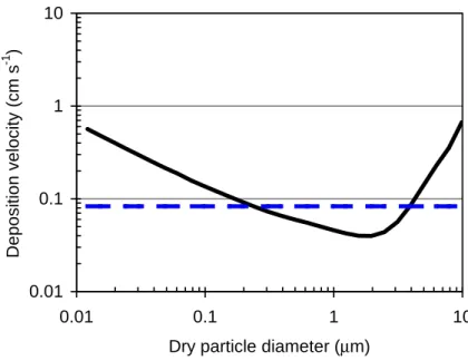
size-dependent scheme of Zhang et al. (2001). For all other species, dry deposition velocities are modeled using the approach of Wesely (1989) as described by Wang et al. (1998). Figure 1 shows annual and global area-weighted average dry deposition velocities as a function of aerosol diameter. For comparison, the original bulk aerosol dry deposition velocity is shown as the straight line.

25

(13)

ACPD

Full Screen / Esc

2.1.6 Wet deposition

Wet deposition in GEOS-CHEM includes three main processes: 1) in-cloud scaveng-ing (rainout), 2) below-cloud scavengscaveng-ing (washout), and 3) scavengscaveng-ing in convective updrafts. In-cloud and below-cloud scavenging are treated separately for stratiform precipitation and convective anvils. Scavenging in convective updrafts represents

re-5

moval in the convective column during vertical transport. Details of the wet deposition scheme used in GEOS-CHEM are described in Liu et al. (2001). Here we discuss the changes made to accommodate size-resolved wet deposition.

In-cloud scavenging, sometimes called “nucleation scavenging”, is treated as a first-order loss utilizing the rainout rate constant computed by Giorgi and Chaimedes (1986).

10

The rate constants are different for stratiform and convective anvil precipitation. We did not modify the original calculation of the rate constant but simply apply the assump-tion, similar to AS02, that only those particles larger than the activation diameter are subjected to removal. The activation diameter for large-scale precipitation is 0.082 µm and for convective precipitation is 0.033 µm. These activation diameters were chosen

15

based on the maximum supersaturations that stratiform and convective clouds typically experience of 0.19% and 0.75%, respectively.

Below-cloud scavenging of gaseous and bulk aerosol species in the original GEOS-CHEM was calculated using a washout rate constant of 0.1 mm−1 of precipitation ap-plied to the precipitating fraction of the grid area (Liu et al., 2001). Here we introduce

20

size-resolved washout in the same way as in AS02. The size-dependent washout rate constants were taken from Fig. 2 of Dana and Hales (1976), which are theoretical washout rate coefficients as a function of aerosol size.

The wet deposition scheme also allows release of scavenged aerosol during oration of precipitation below cloud. The assumption is, for a given fraction f of

evap-25

orating precipitation, only 0.5f of the scavenged aerosol load is released at that level. The 0.5 fraction is to account for a combination of drops that evaporate completely, releasing their entire dissolved aerosol, and drops that partly evaporate and do not

(14)

ACPD

Full Screen / Esc

release any dissolved aerosol (Koch et al., 1999). In the original GEOS-CHEM, the re-evaporating scavenged SO2 is put into the bulk SO4 aerosol assuming it has

un-dergone aqueous oxidation. In this work, we distribute the re-evaporating SO2 over

the aerosol size distribution in the same way as SO₄ produced by standard aqueous oxidation.

5

Scavenging in convective updrafts is calculated by a first-order rate loss where the scavenged fraction is a function of scavenging efficiency and the height of the updraft column. Here we do not make any change to the scavenging fraction calculation. However, we apply the same assumption described above, namely that only activated particles are scavenged. For convective precipitation, these are particles larger than

10

0.033 µm.

2.2 Models for intercomparison 2.3 GISS GCM-II’ model

The GISS GCM-II’ model is a 3-D general circulation model. The TOMAS microphysics has been incorporated into the GISS GCM-II’ and applied to sulfate aerosol as

de-15

scribed in AS02. This work uses the model results from a later version of the GISS GCM-II’ with the addition of sea-salt aerosol (Pierce and Adams, 2006). This version of GISS GCM-II’ has a horizontal resolution of 4◦latitude by 5◦ longitude and 9 sigma-coordinate levels from surface to 10 mb level. GISS sulfur emission in the model is taken from the GEIA 1985 inventory. Specifically, we compare against the “CLRK”

sim-20

ulation of Pierce and Adams (2006), which calculated sea-salt emissions using same Clarke et al. (2006) parameterization adopted here.

Both the GEOS-CHEM model and the GISS GCM-II’ model have similar implemen-tations of TOMAS microphysics, so a major difference is simply their respective mete-orological fields. Additionally, the GISS GCM uses archived monthly average oxidant

25

fields while GEOS-CHEM, in this work, uses the option to calculate and update the oxidant fields simultaneously with photochemistry. Another important difference is the

(15)

ACPD

Full Screen / Esc

treatment of clouds for in-cloud oxidation; GISS GCM-II’ explicitly handles stratiform and convective clouds separately while GEOS-CHEM does not. This leads to different treatments of aerosol activation during aqueous oxidation as described in Sect. 2.1.1. 2.4 GLOMAP model

GLOMAP (GLObal Model of Aerosol Processes) is a size-resolved microphysics model

5

which is an extension to the 3-D offline Eulerian chemical transport model, TOMCAT, described in e.g. Stockwell and Chipperfield (1999). GLOMAP runs on assimilated me-teorology from the European Centre for Medium-Range Weather Forecasts (ECMWF). The spatial resolution of the model grid is 2.8◦latitude by 2.8◦longitude with 31 hybrid sigma-pressure (σ-p) levels extending from the surface to 10mb level. The aerosol

10

size distributions are simulated using the moving-center scheme of Jacobson (1997) and represented by 20 size sections having bin centers spanning 0.003 to 25 µm equiv-alent dry diameters. The details of GLOMAP are described in Spracklen et al. (2005a). The results used in our comparison are from a version of GLOMAP that includes only sulfate and sea-salt aerosols using the GEIA 1985 sulfur emission and the sea spray

15

emission parameterization of Gong (2003). In this version of GLOMAP, oxidant (OH, H₂O₂, etc.) concentrations are specified using monthly mean fields. We use GLOMAP model results from a simulation of year 1996 for our intercomparison.

Although GLOMAP and GEOS-CHEM with the TOMAS microphysics are models developed independently, there are several similarities. Both use assimilated

mete-20

orology. Although different in their details, both the two-moment sectional treatment of TOMAS and the moving center treatment in GLOMAP are high-resolution sectional treatments of the aerosol size distribution that guarantee that both number and mass balance equations are satisfied.

An important difference in GLOMAP microphysics and TOMAS microphysics are

25

their nucleation parameterizations and how they treat the competition between nucle-ation and condensnucle-ation. Both assume binary nuclenucle-ation in the H₂SO₄-H₂O system. While TOMAS uses a critical concentration of H2SO4 as a criterion for nucleation,

(16)

ACPD

Full Screen / Esc

GLOMAP explicitly calculates nucleation rates with the parameterization of Kulmala et al. (1998). Regarding the competition of nucleation and condensation for the avail-able gas phase H2SO4, GLOMAP captures this competition by selecting a short time

step (generally 90 s) for both nucleation and condensation. TOMAS treats the compe-tition in a simpler way as discussed in Sect. 2.1. Another important assumption used

5

in GLOMAP is the activation of particles with dry diameter larger than 0.05 µm.

3 Model predictions

3.1 Sulfate mass prediction

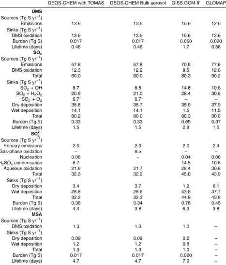
Table 1 presents the sulfur budget calculated from GEOS-CHEM predictions using the size-resolved aerosol model developed in this work compared to the previous bulk

10

aerosol model and the two other microphysics models. Note that evaporating SO2

from cloud droplets is assumed to have been oxidized to SO₄via aqueous chemistry (Sect. 2.1.6) and is, therefore, included in the SO2+H2O2 term in Table 1. Overall,

the sulfur budget in this work changes only slightly with respect to the original GEOS-CHEM with bulk aerosol. The annual-average global burden of sulfate is increased from

15

0.34 Tg S to 0.38 Tg S, and the lifetime is increased from 3.8 to 4.4 days. The imple-mentation of microphysical processes affects the mass burden primarily by changing the depositional sinks. Size-resolved wet deposition, a major sink of sulfate mass and a major change from the bulk aerosol model, affects the sulfate mass budget by slow-ing down wet depositional lifetime by 11%. The major reduction of in-cloud scavengslow-ing

20

only impacts ultrafine mode particles, which are a small portion of the total sulfate mass, while the modification of below-cloud scavenging results in only little change due to the relative unimportance of the below-cloud scavenging. Also, sulfate dry de-position changes only slightly despite the new size-dependent dry dede-position velocities shown in Fig. 1. This is because the predicted sulfate mass distribution is dominated

25

by a mode centering on approximately 0.2 µm. At this size, the new dry deposition 14383

(17)

ACPD

Full Screen / Esc

velocity equals that of the bulk aerosol model; thus the effect of the size-resolved dry deposition is a modest 20% increase in dry depositional lifetime.

3.2 Sea-salt mass prediction

Table 2 presents the sea-salt mass budget from this work in comparison with the ear-lier work by Alexander et al. (2005) and the intercomparison models. The Clarke et

5

al. (2006) emission (this work) produces 78% more sea-salt than that of Monahan et al. (1986) (Alexander et al., 2005). Pierce and Adams (2006) also found the sea-salt emission from the Clarke et al. (2006) parameterization to be more than that from the Monahan et al. (1986) parameterization. Comparing our budget with that from Alexan-der et al. (2005) also highlights the effect of different size-dependent dry deposition

10

treatments, with dry deposition being a dominant sink in their work. Though both ver-sions of GEOS-CHEM have the size-dependent dry deposition scheme of Zhang et al. (2001), which can calculate a dry deposition velocity for any given size, Alexander et al. (2005) only had two modes of sea-salt while our size bins are more resolved, thus experiencing a greater range of deposition velocities. The coarse mode sea-salt

15

in Alexander et al. (2005) is assumed to have a fast dry deposition velocity of a∼10 µm diameter particle. In our work, most of the coarse sea-salt mass centers around 7 µm diameter, with a correspondingly lower dry deposition velocity (see Fig. 1). Conse-quently, their coarse-mode depositional lifetime is 0.7 days compared with 4.9 days in our work. As for wet deposition, we implemented size-dependent wet deposition

cri-20

teria while Alexander et al. (2005) use the original wet deposition for bulk aerosol (Liu et al., 2001). The difference in wet depositional lifetime (50% slower in this work com-pared to Alexander et al., 2005), however, is not mainly due to size-dependent wet deposition but rather to a combination of different precipitation in different simulation years and different locations of emissions. The combined result of these changes is

25

that wet deposition is the dominant sink of coarse mode sea-salt in our sea-salt budget with an overall longer sea-salt lifetime.

(18)

ACPD

Full Screen / Esc

3.3 Aerosol number concentration prediction

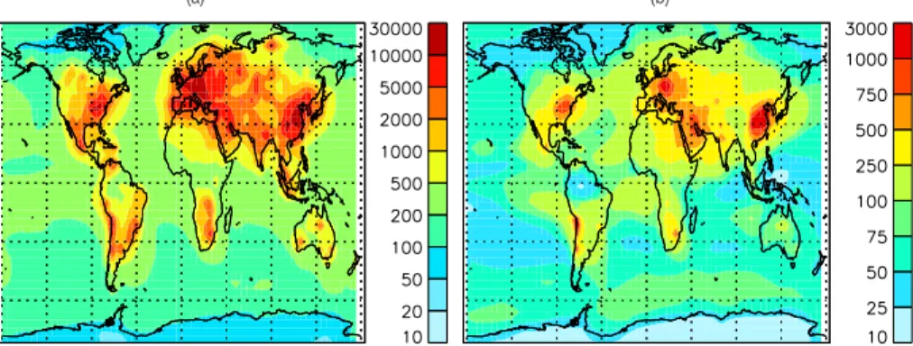
Figure 2 shows the predicted annual average CN and CCN(0.2%) concentrations (cm−3 at STP conditions of 273 K and 1 atm) in the lowest model layer. The CCN at 0.2% supersaturation is calculated as particles with diameter larger than 80 nm, which accu-rately represents the corresponding activation diameter of sulfate, sea-salt, and

mix-5

tures thereof. The predictions show the expected features of high number concentra-tions over land and low over oceans. Predicted CN concentraconcentra-tions exceed 10 000 cm−3 in the most polluted industrialized areas and are within the range of observed values of 5000(Raes et al., 2000b) and 100 000 cm−3(Pandis et al., 1995). Outside the most polluted regions, continental CN concentrations mostly range from 500 to 5000 cm−3.

10

For the marine boundary layer, CN concentrations are 100–500 cm−3, which are com-parable with observations (Andreae et al., 1995; Clarke et al., 1987; Covert et al., 1996; Fitzgerald, 1991; Pandis et al., 1995; Raes et al., 2000b).

For CCN(0.2%) concentrations, the same trend of higher concentration over land than ocean is captured as well. CCN(0.2%) concentrations exceed 1000 cm−3 over

15

the most polluted regions. Typical CCN(0.2%) concentrations over land are 100– 1000 cm−3, while they range only from 10 to 100 cm−3 over oceans in agreement with expected values (Andreae et al., 1995).

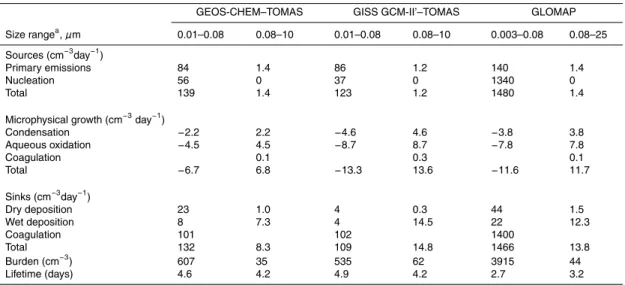
Table 3 presents a global annual aerosol number budget. The size modes are cate-gorized into ultrafine (0.01–0.08 µm) and CCN (0.08–10 µm) modes. Note that

coag-20

ulation is a sink for smaller particles and also a microphysical growth process adding particles into larger size bins, so coagulation is tabulated under both categories in Ta-ble 3. Source contributions to the ultrafine mode from nucleation and primary emission are comparable suggesting potential importance of both sources for CCN production. A major contributor of CCN is growth by aqueous oxidation. Coagulation is the dominant

25

sink of ultrafine aerosols while wet deposition is the dominant sink of CCN.

(19)

ACPD

Full Screen / Esc

3.4 Aerosol size distributions

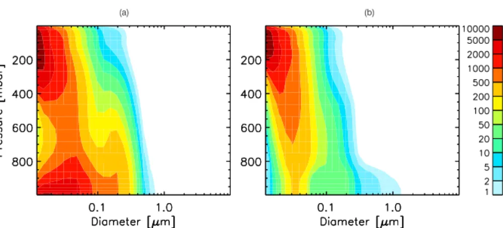
Figure 3 presents vertical profiles of the predicted aerosol number size distribution for two regions: 1) a polluted continental region, Eastern China (100◦E–120◦E, 30◦N– 46◦N) and 2) a clean marine region, the South Pacific Ocean (135◦W–160◦W, 14◦S– 30◦S). Vertical profiles emphasize how primary emissions, nucleation, and different

5

aerosol growth mechanisms impact size distributions at different altitudes. In the upper troposphere, nucleation is the contributor as is evident in both Figs. 3a and 3b with peak ultrafine concentrations of up to 3000 cm−3. The air column over Eastern China shows higher nucleation rates with greater vertical extent than the South Pacific because there is more SO₂ circulating in the northern hemisphere compared to the southern

hemi-10

sphere. In the boundary layer, primary emissions are the dominant source of aerosol number. Primary sulfate emission gives higher ultrafine number concentrations in the polluted continental region in Fig. 3a than the remote marine region in Fig. 3b. Sim-ilarly, primary sea-salt emission influences the size distribution in the Pacific Ocean with lower number concentration overall compared to primary sulfate emission. The

15

bimodal structure in the boundary layer, most noticeable for the remote marine area, can be explained by in-cloud oxidation providing a source of sulfate mass and a growth mechanism for Aitken mode particles to grow to accumulation mode. Sea-salt emission supplies significant mass to the coarse mode in the marine area, which explains the tail of the size distribution extending over 1 µm size range in the remote marine region but

20

not for the continental region. We can observe trends with altitude as nucleated par-ticles grow as they subside. Freshly nucleated parpar-ticles aloft become larger at lower altitudes and finally form a bimodal structure in the cloud-processed BL. Subsidence and entrainment from the FT into the PBL is more important to CCN formation for the MBL than the polluted boundary layer.

25

(20)

ACPD

Full Screen / Esc

4 Comparison with field observations

To test how realistic the model predictions are, model results can be compared with observational data. As a performance benchmark of currently available global models, the IPCC model comparison workshop reported average absolute errors (in percent) of modeled concentrations versus surface observations among different models for each

5

aerosol species, i.e., sulfate (26%), sea-salt (46%), dust (70%), black carbon (179%) and organic carbon (154%) (IPCC, 2001). The COSAM experiment (Barrie et al., 2001) found intermodel differences in surface level seasonal mean of sulfate mixing ratios within 20% and up to a factor of 2 for SO₂ mixing ratios compared to observations. These comparisons show the level of predictive skill among currently available global

10

models for bulk aerosol mass.

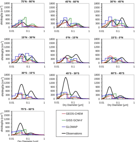
For our model testing, we compare model results with the observational data of Heintzenberg at al. (2000). That data came from a large set of long-term sampling sites and various field campaigns and a variety of sampling instruments. The marine aerosol size distribution measurements were summarized by fitting the data to two

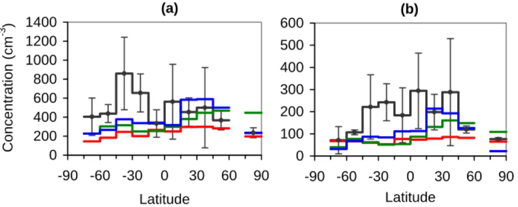
15

lognormal modes for different latitudinal zones. Each latitude band is 15◦wide with no data between 75◦S–90◦S and 60◦N–75◦N. To focus on marine aerosol, we exclude some of our continental grid cell data where it falls in their 15◦×15◦grid area.

Shown in Fig. 4, the bimodal structure of the Heintzenberg at al. (2000) data is captured in the predicted size distributions of all models. An important feature of the

20

size distributions from each model is the minimum between modes, the location of which corresponds directly to the assumed activation diameters in aqueous oxidation (see Sect. 2.1.1). In the case of GISS GCM-II’, as a result of having two activation diameters, three modes appear in the size distributions of some latitudinal bands. The detailed size distributions from the models differ, and no model clearly outperforms the

25

others.

Figure 5a shows the meridional distribution of predicted and observed CN concentra-tions. Global average absolute errors in cm−3(and in percent) of predicted CN are 244

(21)

ACPD

Full Screen / Esc

(45%), 204 (41%), and 176 (32%) cm−3in GEOS-CHEM, GISS GCM-II’, and GLOMAP, respectively. The latitudes where all models fail to predict within the range of the ob-served mean± one standard deviation are 15◦S–60◦S. Over Southern Ocean regions, the marine aerosol should be dominated by sea spray emission when not affected much by carbonaceous aerosols from biomass burning. Therefore the 31%–72%

underpre-5

diction in the 15◦S–60◦S latitude band in all models could be due to either the sea-salt emission or the lack of carbonaceous aerosols. Pierce et al. (2007) explores the re-sult of adding carbonaceous aerosols to a sulfate-sea-salt model in GISS GCM-II’ and found only a minor improvement, reducing model bias in CN prediction from−63% to −38% for 30◦S–45◦S region compared to the same observations.

10

Figure 5b presents a meridional distribution of predicted CCN(0.2%) comparing with observed accumulation mode aerosol (D_p>80 nm) concentrations used as surrogate for CCN(0.2%). Variability ranges are estimated standard deviation values of the accu-mulation mode aerosol shown in Fig. 3 of Heintzenberg at al. (2000). Global average absolute errors in cm−3 (and in percent) of predicted CCN(0.2%) are 109 (50%), 101

15

(51%), and 80 (44%) cm−3 in GEOS-CHEM, GISS GCM-II’, and GLOMAP, respec-tively. Overall, we find that all three models have encouragingly high skill in predicting CN and CCN(0.2%) concentrations in the marine boundary layer, with average errors in the 30%–50% range, comparable to global model skill for predicting sulfate and sea-salt mass concentrations and much better than carbonaceous or mineral dust mass

20

concentrations.

5 Model intercomparison

In this section, we compare GEOS-CHEM predictions with those from GISS GCM-II’ and GLOMAP. The goal is to observe model behaviors and the level of agreement or disagreement, keeping in mind that the results are not from the same simulation year.

25

The focus of this intercomparison is on CN and CCN predictions.

(22)

ACPD

Full Screen / Esc

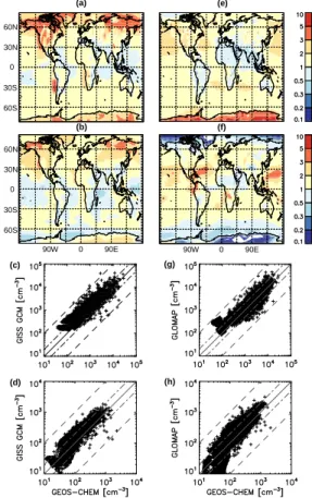
5.1 Surface Predictions

We compare the predicted surface CN and CCN(0.2%) concentrations from the GISS GCM-II’ and the GLOMAP models to those from GEOS-CHEM in terms of concen-tration ratios as shown in Fig. 6. The latitude-longitude map shows the spatial dis-tribution of concentration ratios while the scatter plots present the level of agreement

5

with GEOS-CHEM. Over the southern part of Europe and Asia, GEOS-CHEM predicts higher CN concentrations compared to both GLOMAP and GISS GCM-II’. This is be-cause, among these models, only GEOS-CHEM uses the sulfur emission inventory with updated national emission and fuel use data. Although SO₂ emissions globally and from developed countries are lower in the updated inventory, emissions from

de-10

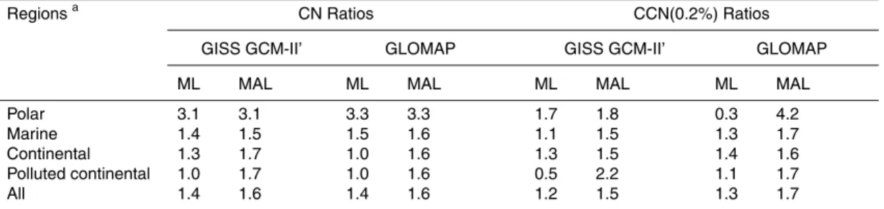
veloping countries such as Thailand, Indonesia, Turkey, and Pakistan have increased by factors of 2 to 3 in 2000 with respect to 1985. Figure 6 also presents scatter plots comparing surface CN and CCN(0.2%) predictions from model pairs. Comparisons of GEOS-CHEM against GISS GCM-II’ and GLOMAP do not exhibit significantly different trends except in specific regions, e.g. CCN(0.2%) in polar regions.

15

The level of agreement of surface prediction is summarized in Table 4 as area-weighted mean log (ML) of ratios and mean absolute log (MAL) of ratios, which are calculated as follows, log ML = 1 N N X i=1 log x_i (1) and 20 log MAL = 1 N N X i=1 |log xi| (2)

where xi is a ratio of concentrations from a model pair at grid box i and N is the number of grid boxes. The ratios are categorized into four different regions based on the CN and CCN(0.2%) concentrations predicted by GEOS-CHEM. The resulting regions can

(23)

ACPD

Full Screen / Esc

be loosely described as “polluted continental”, “continental”, “marine”, and “polar”. ML of ratios is indicative of the ratio of burden over the domain of interest, e.g. the surface, while MAL suggests the level of agreement between two models on average and MAL of 1.0 means perfect agreement. MAL of ratios of both CN and CCN(0.2%) fall within a factor of 2 except for over the poles in both models. Differences of predictions among

5

models could be purely due to different wind fields distributing the same total amount; however, this is not the case. On average, the ML results show that both GISS GCM-II’ and GLOMAP predict 40% higher surface CN concentrations compared to CHEM. For surface CCN(0.2%), GISS GCM-II’ and GLOMAP, compared with GEOS-CHEM, predict 20% and 30% higher concentrations on average, respectively. Lower

10

concentrations of both CN and CCN(0.2%) in GEOS-CHEM are attributable to the use of updated emission inventories with lower sulfur emissions.

Table 4 shows that GEOS-CHEM CCN(0.2%) predictions are slightly closer to those from the GISS GCM II’ than GLOMAP. Otherwise, despite sharing the common TOMAS aerosol microphysics, the overall differences between GEOS-CHEM and GISS GCM II’

15

are generally as large as the differences between GEOS-CHEM and GLOMAP. There-fore, the intercomparison does not show obvious behaviors influenced by meteorology or aerosol microphysics alone but suggests that meteorological fields are as important to the aerosol number predictions as model chemistry and microphysical schemes. Also the differences are higher on a monthly average basis (not shown), which

rein-20

forces the need to simulate accurately at specific times using the assimilated meteo-rology.

5.2 Zonal average predictions

Figure 7 shows the annual and zonal average CN (D_p>10 nm) and CCN(0.2%) pre-dictions at STP conditions from the three models and zonal average nucleation mode

25

(1–10 nm) concentrations from GLOMAP. For GEOS-CHEM results, we only show pre-dictions below the annual average tropopause above which aerosol microphysics was not simulated. For CN concentrations, features evident in all models are the elevated

(24)

ACPD

Full Screen / Esc

CN concentrations in the upper troposphere because of nucleation and the high CN from surface primary emissions centering at about 40◦N–50◦N. The low temperatures, low particle surface area, and high relative humidity in the equatorial upper troposphere create ideal conditions for binary nucleation. However, while all models predict high CN concentrations in the upper troposphere because of nucleation, there are differences in

5

the locations and magnitudes of the peak concentrations. All models exhibit major nu-cleation in the equatorial upper troposphere, while GLOMAP also shows its maximum nucleation region extending to the northern mid-latitudes, as shown in Fig. 7g. Also, the peak CN occurs at different altitudes for each model, i.e. 150 and 100 mbar for GEOS-CHEM and GISS GCM-II’, respectively, and 100 and 300 mbar for GLOMAP. In Fig. 7a,

10

GEOS-CHEM predicts high CN concentration across the tropopause spreading into the stratosphere unlike CN predicted by GLOMAP, in which the high concentrations are confined by the tropopause being higher over the equator and descending toward both poles (Fig. 7c and Fig. 7g).

For CCN(0.2%) concentrations, GEOS-CHEM predicts the most widespread and

15

deepest CCN(0.2%) minimum in the tropical upper troposphere, shown in Fig. 7d. The low aerosol surface area in this region contributes to the higher nucleation rates and CN concentrations already mentioned in Fig. 7a. GISS GCM-II’ has the tendency to trans-port heavily polluted air toward the North Pole as evidenced by the higher CCN(0.2%) concentrations there.

20

Similar to other aerosol model intercomparisons, model-model differences increase as one moves upward from the surface. In the free troposphere, predicted CN and CCN(0.2%) concentrations among models can differ by an order of magnitude or more. For example, at 300 mb level (not shown) GISS GCM-II’ compared against GEOS-CHEM has the MAL of ratios of CCN(0.2%) of 2.8 and a maximum ratio of 20 with

25

a large region of high values (>10) over India and a region of low values (<0.1) over Southeast Asia. Similarly, the MAL of CCN(0.2%) ratios of GLOMAP to GEOS-CHEM predictions at 300 mb is 2.3 with a maximum of 15.5.

(25)

ACPD

Full Screen / Esc

5.3 Global Budgets

Analyzing global aerosol mass and number budgets provides some insights into how factors such as meteorology, microphysics, and chemistry, affect the prediction of CN and CCN concentrations and their lifetimes. Tables 1, 2, and 3 present global annual budgets of sulfur, sea-salt, and aerosol number, respectively, from each model in our

5

model intercomparison.

The sulfur budgets in Table 1 show that, for all of the sulfur-containing species, GISS GCM-II’ has higher burdens and longer lifetimes than those of GLOMAP and GEOS-CHEM. For sulfate, all models have similar source contribution profiles (percentage of each source) although GISS GCM-II’ shows slightly more condensation. Comparison

10

of sea-salt budgets in Table 2 points to discrepancies due to meteorology and dry depo-sition schemes. Because GEOS-CHEM and GISS GCM-II’ use the same emissions pa-rameterization, total sea-salt emissions in each model represents the average strength of their winds. Regarding dry deposition, GEOS-CHEM’s coarse-mode dry deposition is significantly slower than other models; dry deposition lifetime of GEOS-CHEM, GISS

15

GCM-II’, and GLOMAP are 4.9, 0.9, and 0.1 days, respectively. Coarse-mode dry de-position velocities in our work are around an order of magnitude smaller than those in GISS GCM-II’, hence the slower dry deposition. The size-dependent dry deposition scheme in GLOMAP is the same as GEOS-CHEM. Therefore, the difference results from different sea-salt size distributions of the respective emissions parameterizations

20

combined with GLOMAP’s inclusion of particles up to 25 µm leading to greater range of dry deposition velocities (see trend in Fig.1). Global budgets show that GEOS-CHEM has the highest sea-salt burden among all models, although the contribution to global CCN(0.2%) is modest since the majority of sea-salt mass is in the coarse-mode and translates to few particles.

25

Presented in Table 3, in this intercomparison, GEOS-CHEM predicts the lowest global-average CCN(0.2%) concentration (burden) of 35 cm−3 compared to 62 and 44 cm−3 in GISS GCM-II’ and GLOMAP, respectively. For ease of interpretation, the

(26)

ACPD

Full Screen / Esc

global burden has been converted to concentration using a tropospheric volume based on an average tropopause height of 12 km. The aerosol number budget shows that GEOS-CHEM has approximately a factor of 2 lower microphysical growth compared to other models, which is the reason for low global CCN(0.2%). Moreover, effective scavenging in the tropical convection in GEOS-CHEM contributes to low tropical UT

5

CCN(0.2%) shown in Fig. 7d. Globally averaged, however, GEOS-CHEM has slower removal compared to other models; wet depositional lifetimes of CCN(0.2%) are 4.8, 4.3, and 3.6 days for GEOS-CHEM, GISS GCM-II’, and GLOMAP, respectively. Low microphysical growth in GEOS-CHEM is attributable to it having the lowest available sources of sulfate, both gas and aqueous phase. In Table 1, total SO2 oxidation

10

sinks, the source of sulfate for microphysical growth, are 30.3, 43.0, and 41.4 Tg S yr−1 in GEOS-CHEM, GISS GCM-II’, and GLOMAP, respectively. The higher nucleation source in GEOS-CHEM than in GISS GCM-II’ shown in Table 3, despite the lower source from SO2+OH, reinforces the finding that there are fewer existing particles in

the upper equatorial troposphere.

15

CCN lifetimes (Table 3) of 4.2, 4.2, and 3.2 days for GEOS-CHEM, GISS GCM-II’, and GLOMAP, respectively, are comparable. For particles smaller than 0.08 µm, GEOS-CHEM and GISS GCM-II’ predict very close lifetimes as well. Not surprisingly, GLOMAP has a much shorter lifetime of 2.7 days for ultrafine particles than the other two models; given that GLOMAP’s lower size limit includes smaller particles in the

20

1–10 nm size range, their ultrafine particles are subjected to very fast coagulation.

6 Discussion and conclusions

The size-resolved aerosol microphysics module, TOMAS, has been introduced to the GEOS-CHEM chemical-transport model. Because GEOS-CHEM is driven by assimi-lated meteorology, it will be an ideal vehicle for testing the TOMAS microphysics

simu-25

lation, especially against field campaign data. Advantages of a two-moment sectional method are high size resolution, accurate and efficient representation of both mass

(27)

ACPD

Full Screen / Esc

and number, and conservation of aerosol number, which are essential to our ultimate goal of improving the indirect radiative forcing estimates. Microphysical processes in-clude condensation/evaporation, coagulation, and nucleation. Apart from introducing microphysical processes to the model, existing processes, namely emission, advection, convection, chemistry, and deposition, were modified to handle aerosol size

distribu-5

tions properly. The aerosol size distribution is represented by size bins segregated by dry aerosol mass covering the range of about 10 nm to 10 µm dry diameter. Sulfate and sea-salt aerosols are included in the current microphysics model.

Qualitative features of atmospheric aerosols are well simulated, e.g. higher aerosol concentrations over land than oceans, the nucleation dominated size distribution in the

10

upper troposphere, the primary emission dominated size distribution over source re-gions at surface, and the bimodal size distribution over the MBL resulting from in-cloud sulfur oxidation. Additionally, as a benchmark for the current state of global micro-physics model development, we perform a model intercomparison with GISS GCM-II’ and GLOMAP models, which are global models with two-moment aerosol

micro-15

physics. A comparison of annual-average MBL CN and CCN(0.2%) predictions from each model to a compilation of MBL aerosol observations of Heintzenberg at al. (2000) show reasonably good predictive skill with annually averaged absolute errors of 30– 50%. However, all models underpredict CN and CCN(0.2%) over the Southern Ocean by 45–57% suggesting a common point for improvement in sea-salt emissions.

More-20

over, all overpredict CN concentrations between 45◦ and 60◦N suggesting potential weakness in the common sulfate primary emission. Overall, model skill for predict-ing CN and CCN(0.2%) is comparable with global model skill in predictpredict-ing sulfate and sea-salt mass and much better than those predicting carbonaceous aerosols and dust mass.

25

Model intercomparison at the surface shows agreement generally within a factor of 2 for CN and CCN(0.2%) predictions except over the poles; GISS GCM-II’ and GLOMAP on average predict CN and CCN(0.2%) within 60% and 50%–70% to GEOS-CHEM prediction, respectively. Major differences at the surface are due to different transport

(28)

ACPD

Full Screen / Esc

and emissions. GEOS-CHEM also predicts lower surface concentrations of CN and CCN(0.2%) than the other two models. Zonal average comparison reveals discrepan-cies in location and concentration of peak CN in the upper troposphere that is a feature of nucleation. Global annually averaged budgets show that GEOS-CHEM predicts low-est CCN(0.2%) among the three models due to a factor of 2 lower microphysical growth

5

than other models. The level of agreement of each model paired with GEOS-CHEM in this intercomparison suggests that meteorological differences are as significant as differences from chemistry and microphysical schemes. This emphasizes the need to have accurate meteorology that will enable comparison with observations and evalu-ation of aerosol microphysical model. Future work will add other aerosol species to

10

GEOS-CHEM’s microphysical simulation. Then aerosol predictions can be tested with field campaign observations such as the ACE-Asia experiment, which will potentially lead to improvement in our simulation of the aerosol microphysics and ultimately the estimate of the aerosol indirect effects.

Acknowledgements. We thank J. Pierce for providing model results and support on the

anal-15

ysis. We also want to thank R. Park and B. Yantosca for supports on GEOS-CHEM model. This work was supported by funding from the National Aeronautics and Space Administration (Award NNG04GE86G) and from The Office of The Civil Service Commission under The Royal Thai Government.

References

20

Adams, P. J. and Seinfeld, J. H.: Disproportionate impact of particulate emissions on global cloud condensation nuclei concentrations, Geophys. Res. Lett., 30, 2003.

Adams, P. J. and Seinfeld, J. H.: Predicting global aerosol size distributions in general circula-tion models, J. Geophys. Res.-Atmos., 107, 2002.

Albrecht, B. A.: Aerosols, Cloud Microphysics, and Fractional Cloudiness, Science, 245, 1227–

25

1230, 1989.

Alexander, B., Park, R. J., Jacob, D. J., Li, Q. B., Yantosca, R. M., Savarino, J., Lee, C. C.

(29)

ACPD

Full Screen / Esc

W., and Thiemens, M. H.: Sulfate formation in sea-salt aerosols: Constraints from oxygen isotopes, J. Geophys. Res.-Atmos., 110, 2005.

Andreae, M. O., Elbert, W., and Demora, S. J.: Biogenic Sulfur Emissions and Aerosols over the Tropical South-Atlantic .3. Atmospheric Dimethylsulfide, Aerosols and Cloud Condensation Nuclei, J. Geophys. Res.-Atmos., 100, 11 335–11 356, 1995.

5

Barrie, L. A., Yi, Y., Leaitch, W. R., Lohmann, U., Kasibhatla, P., Roelofs, G. J., Wilson, J., McGovern, F., Benkovitz, C., Melieres, M. A., Law, K., Prospero, J., Kritz, M., Bergmann, D., Bridgeman, C., Chin, M., Christensen, J., Easter, R., Feichter, J., Land, C., Jeuken, A., Kjellstrom, E., Koch, D., and Rasch, P.: A comparison of large-scale atmospheric sulphate aerosol models (COSAM): overview and highlights, Tellus B, 53, 615–645, 2001.

10

Bates, T. S., Huebert, B. J., Gras, J. L., Griffiths, F. B., and Durkee, P. A.: International Global Atmospheric Chemistry (IGAC) project’s first aerosol characterization experiment (ACE 1): Overview, J. Geophys. Res.-Atmos., 103, 16 297—16 318, 1998.

Bates, T. S., Quinn, P. K., Coffman, D. J., Johnson, J. E., Miller, T. L., Covert, D. S., Wieden-sohler, A., Leinert, S., Nowak, A., and Neususs, C.: Regional physical and chemical

proper-15

ties of the marine boundary layer aerosol across the Atlantic during Aerosols99: An overview, J. Geophys. Res.-Atmos., 106, 20 767–20 782, 2001.

Bey, I., Jacob, D. J., Yantosca, R. M., Logan, J. A., Field, B. D., Fiore, A. M., Li, Q. B., Liu, H. G. Y., Mickley, L. J. and Schultz, M. G.: Global modeling of tropospheric chemistry with assimilated meteorology: Model description and evaluation, J. Geophys. Res.-Atmos., 106,

20

23 073–23 095, 2001.

Boucher, O. and Lohmann, U.: The Sulfate-CCN-Cloud Albedo Effect – a Sensitivity Study with 2 General-Circulation Models, Tellus B, 47, 281–300, 1995.

Carpenter, R. L., Droegemeier, K. K., Woodward, P. R., and Hane, C. E.: Application of the Piecewise Parabolic Method (PPM) to Meteorological Modeling, Mon. Weather. Rev., 118,

25

586–612, 1990.

Charlson, R. J., Schwartz, S. E., Hales, J. M., Cess, R. D., Coakley, J. A., Hansen, J. E., and Hofmann, D. J.: Climate Forcing by Anthropogenic Aerosols, Science, 255, 423–430, 1992. Chin, M., Rood, R. B., Lin, S. J., Muller, J. F., and Thompson, A. M.: Atmospheric sulfur

cycle simulated in the global model GOCART: Model description and global properties, J.

30

Geophys. Res.-Atmos., 105, 24 671–24 687, 2000.

Clarke, A. D., Ahlquist, N. C., and Covert, D. S.: The Pacific Marine Aerosol – Evidence for Natural Acid Sulfates, J. Geophys. Res.-Atmos., 92, 4179–4190, 1987.