HAL Id: hal-00302887
https://hal.archives-ouvertes.fr/hal-00302887
Submitted on 27 Jul 2007
HAL is a multi-disciplinary open access
archive for the deposit and dissemination of
sci-entific research documents, whether they are
pub-lished or not. The documents may come from
teaching and research institutions in France or
abroad, or from public or private research centers.
L’archive ouverte pluridisciplinaire HAL, est
destinée au dépôt et à la diffusion de documents
scientifiques de niveau recherche, publiés ou non,
émanant des établissements d’enseignement et de
recherche français ou étrangers, des laboratoires
publics ou privés.
Long-range correlations of extrapolar total ozone are
determined by the global atmospheric circulation
P. Kiss, R. Müller, I. M. Jánosi
To cite this version:
P. Kiss, R. Müller, I. M. Jánosi. Long-range correlations of extrapolar total ozone are determined by
the global atmospheric circulation. Nonlinear Processes in Geophysics, European Geosciences Union
(EGU), 2007, 14 (4), pp.435-442. �hal-00302887�
© Author(s) 2007. This work is licensed
under a Creative Commons License.
in Geophysics
Long-range correlations of extrapolar total ozone are determined by
the global atmospheric circulation
P. Kiss1, R. M ¨uller2, and I. M. J´anosi1
1Department of Physics of Complex Systems, E¨otv¨os University, Budapest, Hungary 2ICG-1, Research Centre J¨ulich, Germany
Received: 24 April 2007 – Revised: 27 June 2007 – Accepted: 25 July 2007 – Published: 27 July 2007
Abstract. TOMS (Version 8) ozone records are analysed
between latitudes 60◦S and 60◦N, in order to extract au-tocorrelation properties with high spatial resolution. After the removal of semi-annual, annual, and quasi-biennial back-ground oscillations, the residuals are evaluated by detrended fluctuation analysis. Long-range correlations are detected ev-erywhere. Surprisingly, the latitude dependence of zonally averaged correlation exponents exhibits the same behaviour as the exponents for daily surface temperature records. This suggests that the correlation properties of total ozone column are dominated by the global atmospheric circulation patterns, and the effect of chemical processes seems to be subsidiary.
1 Introduction
There is a widespread interest in understanding the proper-ties and dynamics of atmospheric ozone. Special attention is paid to the observed slow decline of the total amount of stratospheric ozone in the past decades, and the strong sea-sonal depletion over the polar regions known as ozone hole (e.g., Weatherhead and Andersen, 2006; WMO, 2007). In recent years, the question how a recovery of stratospheric ozone can be detected and attributed to the observed de-cline of the halogen loading has attracted considerable in-terest (WMO, 2007). The chemistry affecting stratospheric ozone is today largely understood and, likewise, the general mechanisms are known that determine the impact of dynam-ics on total column ozone (TO). Nonetheless, a reproduction of the interplay between chemistry and dynamics and the re-sulting ozone levels in models still constitutes a consider-able challenge (Eyring et al., 2006) and extracting the chem-ical contribution to observed ozone trends is difficult (WMO, 2007). Deducing correlation properties from measured data
Correspondence to: I. M. J´anosi
is a starting step to characterise the dynamics, and has also relevant implications in trend analysis (Vyushin et al., 2007). The Total Ozone Mapping Spectrometers (TOMS) have been a successful series of instruments designed for measur-ing TO, and providmeasur-ing other products such as the aerosol index, reflectivity, ultraviolet radiation, and volcanic SO2
(http://toms.gsfc.nasa.gov/). Here we present a detailed anal-ysis for two TO data sets collected on the satellites Nimbus-7 (N7) in the period 1 November 1978–6 May 1993, and Earth-Probe (EP) between 25 July 1996 and 30 Dec. 2005. We use the method of detrended fluctuation analysis (DFA) (Peng et al., 1994, 1995), which is able to eliminate slow trends from long nonstationary signals. The proper technique is crucial, especially because instrumental problems were de-tected in early 2001, and a warning was released that EP-TOMS data past mid 2000 should not be used for trend anal-ysis (http://toms.gsfc.nasa.gov/news/news.html).
In the next Section we give details on the data and meth-ods. Special care is taken to remove the quasi-biennial os-cillations (QBO) from the signals, because such background cycles are known to distort correlation exponents (J´anosi and M¨uller, 2005). Then we present a detailed map of exponent values and comparison with existing results for other meteo-rological variables. We argue that the correlation properties of the total ozone time series suggest the dominance of dy-namical processes, thus TO outside the polar regions over a given geographic location can be considered as a “passive” scalar, similarly to temperature.
2 Data and methods
The TOMS instruments measure backscattered ultraviolet ra-diation at six wavelengths, and provide a contiguous grid-ded mapping of TO with a spatial resolution of 1.0◦×1.25◦ (lat/long). In order to minimise the effects of known instru-mental distortions at high solar zenith angles and missing
436 P. Kiss, R. M¨uller and I. M. J´anosi: Long-range correlations of TOMS total ozone 280 290 300 310 TO [DU] 1980 1985 1990 1995 2000 2005 year 103 104
# of observations Nimbus-7 Earth-Probe
(a)
(b)
Fig. 1. (a) Daily mean total ozone (in Dobson units) averaged in the band 60◦S and 60◦N latitude for the TOMS data bank. (b) Number of daily observations for the Nimbus-7 and Earth-Probe satellites (note the logarithmic vertical scale).
0 100 200 300 day of year 260 280 300 320 340 mean TO [DU] 0 100 200 300 day of year
(a) Nimbus-7 (b) Earth-Probe
Fig. 2. Annual cycle of daily mean total ozone (TO) averaged over 0◦–60◦N lat (northern hemisphere, black symbols) and 0◦–60◦S lat (southern hemisphere, white symbols) for (a) N7-TO, and (b) EP-TO. Gray bands indicate one sigma standard deviations.
polar night intervals, data evaluation is restricted between lat-itudes 60◦S and 60◦N covering ∼ 87% of the earth surface. Daily average TO values over this band are plotted in Fig. 1a, the number of observations is shown in Fig. 1b.
Figure 2 illustrates the daily mean TO levels averaged sep-arately over the northern and southern hemispheres, for a given calendar day. The total column ozone has very sim-ilar annual cycles for both satellite records (apart from the clear baseline drop of EP data), the different amplitudes and phase shift between the hemispheres explain the net annual periodicity visible in Fig. 1a.
Since a reasonable application of DFA requires the re-moval of all dominant periodicities, we have performed a de-tailed spectral analysis of TO time series for each geographic location. We have implemented the Lomb periodogram al-gorithm (Press et al., 1992) in order to properly treat missing
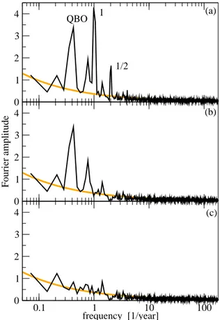
0 1 2 3 4 0 1 2 3 4 Fourier amplitude 0.1 1 10 100 frequency [1/year] 0 1 2 3 4 (a) (b) (c) 1/2 1 QBO
Fig. 3. Unnormalised power spectrum as a function of frequency (note the logarithmic scale) for the geographic location 0.5◦N, 0.625◦E. (a) N7 signal. (Leading period lengths are labelled.) (b) N7 signal after removing the annual periodicities. (c) N7 signal after Wiener filtering for QBO. Orange lines indicate a power-law background with an exponent –1/2.
data points. The spectra for a given geographic location are very similar for both instruments. Since the EP records are shorter, somewhat higher noise level and peak broadening are experienced. Nevertheless the main features are retained for both satellite measurements: the dominant periodicities are semi-annual, annual, and quasi-biennial (Fig. 3a). The TO levels are known to be affected also by the solar cycle of ∼11 years (Hood, 1997; Calisesi and Matthes, 2006), how-ever the TOMS records are too short and the amplitude of the solar signal is too low for a direct detection by Fourier methods.
As a first step of filtering, the annual periodicity is re-moved from the daily values TOi by the long-time climato-logical mean hTOid for the given calendar day d=1 . . . 365 (leap days are omitted) to get the ozone-anomaly series TOai=TOi−hTOid. This procedure cannot remove smeared oscillations from the records, such as QBO (Fig. 3b) or a gradual shift of the annual means. In order to remove the QBO background as well, the Wiener filter method (Press et
(a)
(c)
(b)
(d)
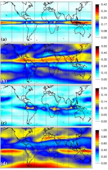
Fig. 4. Geographic distribution of the N7 spectral peak intensities indicated in Fig. 3: (a) QBO peak(s) between 2 and 3 years; (b) Annual peak (1±0.1 year); (c) semi-annual peak (0.5±0.05 year); (d) the continuum background (total area minus the area under the three peaks). Each individual power spectrum is normalised, note the different colour scales.
al., 1992; Hegger et al., 1999) is used by cutting the spectral amplitudes to base-line values in the interval of periods 1.1-4.3 years. The result for an equatorial location is shown in Fig. 3c.
The relative peak heights at the different characteristic fre-quencies (Fig. 3a) depend on the geographic location. The spectral intensity of the semi-annual, annual, and QBO com-ponents is estimated by integrating the area under the peaks of normalised spectra. The map in Fig. 4a illustrates that QBO is almost negligible away from the equator by ∼10◦ latitude. Fig. 4b reveals a marked asymmetry between the hemispheres regarding the strength of annual periodicity, which is also clear in Fig. 2. Similar north-south asymme-try is reflected in the semi-annual periodicities (Fig. 4c). It is quite remarkable that large areas exhibit very weak
peri-odicities (Fig. 4d), especially over the South Atlantic Basin. Note that maps for Earth-Probe data show very similar fea-tures with negligible differences, therefore we use only the (longer) Nimbus-7 record for visualisation.
As a next step, the Wiener filtered ozone-anomaly series are evaluated by DFA procedure. The method is described in hundreds of papers (http://www.physionet.org/physiotools/ dfa/citations.shtml), therefore here we settle for a very short summary. The integrated anomaly time series (so called pro-file) is divided into nonoverlapping segments of equal length n. In each segment, the local trend is fitted by a polyno-mial of order p and the profile is detrended by subtracting this local fit. The strength of fluctuations is measured by the standard deviation in the detrended segment averaged over all the segments hFp(n)i. A power-law relationship between hFp(n)i and n indicates scaling with an exponent δ
(DFA-p ex(DFA-ponent): hF(DFA-p(n)i∼nδ. Notice that such a process has a
power-law autocorrelation function A(τ ) and a power spec-trum S(f )
A(τ ) ∼ τ−α , S(f ) ∼ f−β , (1)
where stationarity requires 0<α<1 and 0<β<1, τ is the usual time lag and f is the frequency variable of the Fourier transform. The relationships between the correlation expo-nents are (Koscielny-Bunde et al., 1998; Talkner and Weber, 2000)
α = 2(1 − δ) , β = 2δ − 1 . (2)
Processes of long-range temporal correlations and finite vari-ance are characterised by DFA exponents 1>δ>1/2, uncor-related time series (e.g., pure random walk) obey δ=1/2. Signals with δ<1/2 are called antipersistent, expressing the behaviour that an increasing trend in the past implies a de-creasing trend in the future, and vice versa.
Local polynomial fits of order p eliminate polynomial background trends of order p − 1, thus DFA-1 does not re-move any incidental nonstationarity, DFA-2 can discard slow linear trends, etc. Long-range correlation is inferred for a given time series when the exponent δ does not depend on p. After checking that both N7 and EP filtered ozone-anomalies obey long-range dependence, an important result by Chen et al. (2002) can be exploited in order to improve the statistics. Namely, if a record has positive long-range corre-lations (δ>1/2), segments up to 50% of the total length can be removed. DFA tests on the rest stitched together show the same scaling behaviour as the whole record. Based on this finding, we merged the N7 and EP filtered anomaly series for a given location resulting in record lengths around 23 years. An example for DFA scaling is shown in Fig. 5.
An essential practical limitation of the DFA method is that the maximal segment size can not be longer than roughly one quarter of the total length. This has the consequence that scaling can be rigorously established only up to timescales for a few years for TO data. Still, the DFA curves similar to
438 P. Kiss, R. M¨uller and I. M. J´anosi: Long-range correlations of TOMS total ozone 0.5 1 1.5 2 2.5 3 log10(n) 1 2 3 log 10 [F(n)] 0.77 0.5
Fig. 5. DFA curves for the filtered and merged data (see text) with linear (black), parabolic (blue), cubic (red), and fourth order poly-nomial (green) local detrending. Characteristic slopes are indicated. (51.5◦N, 110.625◦E).
Fig. 5 do not show a systematic breakdown at a well defined threshold time, apart from steeply increasing irregular fluc-tuations for too large n values. Therefore we use the term “long-range correlation” to indicate the scaling behaviour of DFA curves over the intervals permitted by the record lengths of the time series, and we do not mean that the fluctuations have an infinite memory.
In a recent paper, Vyushin et al. (2007) determined the global correlation properties of TO signals from the same TOMS (version 8) data base. Since their results are quite dif-ferent from ours (see below), here we summarise the most essential steps of their procedure. Instead of daily data, they evaluated time series of zonal and gridded (10◦ lati-tude by 30◦longitude grid) monthly mean total ozone val-ues. Ground based TO measurements were used to fill the gap (see Fig. 1) to obtain nearly continuous time series of 324 monthly mean values. The deterministic part was sepa-rated by multilinear regression of 20 coefficients in a spec-tral decomposition model representing the long term aver-age, seasonal cycle, QBO, solar flux, and a long term trend. The long term trend was described by two different methods, a piecewise-linear trend and the equivalent effective strato-spheric chlorine (EESC) time series. EESC is a measure de-signed to quantify the combined effect of halogens (chlorine and bromine) on ozone depletion in the stratosphere (e.g., Newman et al., 2007; WMO, 2007).Hurst exponents were estimated by computing the power spectra for the residuals, and fitting a power-law for the low frequency part between 1 and 27 years with either a maximum likelihood method or a log-linear regression of the periodogram. Note that the Hurst exponent is mathematically equivalent with the DFA expo-nent δ for an infinite time series, however they can numeri-cally differ for a finite data set (Pilgram and Kaplan, 1998).
(b)
(a)
Fig. 6. (a) Fitted DFA-3 (cubic local detrending) exponent values for the ozone anomaly records for each grid point. (b) Residual percentage variance 100(1–r2) for the linear regression of DFA-3 curve (see Fig. 5) at each grid point.
3 Results
We preformed a DFA analysis for the filtered and merged N7-EP records for each grid point between 65◦S and 65◦N latitudes in the TOMS data base. (This band is little wider than the maps shown, in order to compare the results with temperature data, see below.) Since we could not check vi-sually all the 37 440 individual curves for occurrent residual anomalies, we extracted the DFA-3 slopes of cubic local de-trending which eliminates any contingent linear or quadratic tendency from the data. The results are shown in Fig. 6a. The quality of exponents is visualised in Fig. 6b by com-puting the regression coefficient r for the linear fits on the double-logarithmic DFA-3 curves (c.f., Fig. 5), and plotting the residual percentage variance 100(1 − r2) by colour cod-ing. The unstructured patchy map suggests that the dominant source of errors is statistical fluctuations as a consequence of restricted record lengths, indeed.
The main feature of the geographic distribution of expo-nent values (Fig. 6a) is the marked belt of strong correla-tions between ∼20◦S and 20◦N latitudes. 866 grid points (∼2.5%) have fitted exponent values slightly larger than 1 (the absolute maximum is 1.09 ± 0.04), which indicates that our filtering method is not perfect (we have no reason to as-sume that TO fluctuations obey infinite variance). The ab-solute minimum value is 0.57±0.03, therefore each record exhibits long-range correlations.
The strength of correlations has negligible seasonality. This we checked by the method of “cutting and stitching” (Chen et al., 2002) separately for the summer and winter half-years (1 June–30 November, and 1 December–31 May). The
maps similar to Fig. 6a do not show systematic differences, the overall pattern is the same in both half-years.
Atmospheric variables commonly exhibit long-range asymptotic correlations. Besides the detailed investigation of terrestrial and sea surface temperature records (Pelletier, 1997; Koscielny-Bunde et al., 1998; Talkner and Weber, 2000; Kantelhardt et al., 2001; Weber and Talkner, 2001; Kir´aly and J´anosi, 2002; Blender and Fraedrich, 2003; Eich-ner et al., 2003; Fraedrich, 2003; Fraedrich and Blender, 2003; Fraedrich et al., 2003; Monetti et al., 2003;
Pattanty´us-´
Abrah´am et al., 2004; Kir´aly and J´anosi, 2005; Bartos and J´anosi, 2006; Huybers and Curry, 2006; Kir´aly et al., 2006; Rybski et al., 2006), power-law autocorrelation detected for pressure height fluctuations (Tsonis et al., 1999), total ozone level (Toumi et al., 2001; J´anosi and M¨uller, 2005; Vyushin et al., 2007) or carbon-dioxide (Patra et al., 2006), only to mention a few. Since we have data for daily mean temper-ature correlations, we can directly compare them with the present results for TO. The maps of exponent distributions for temperature show much more complicated patterns (Bar-tos and J´anosi, 2006; Kir´aly et al., 2006), therefore we de-termined the zonal averages for both sets of exponents. The result is shown in Fig. 7a.
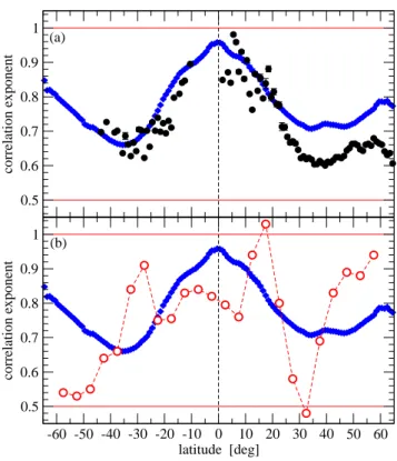
The agreement of zonally averaged correlation exponents for daily surface temperature and TO is quite striking. One might expect much higher variablity for temperature data, since local factors (topography, land coverage, vertical con-vection, etc.) obviously affect strongly how the temperature fluctuates at 2 m height. The variation of TO levels, in con-trast, reflects changes mostly in the lower stratosphere, where ozone concentration is the highest. And indeed, the vari-ability of the correlation exponents with longitude is much stronger for temperature (Bartos and J´anosi, 2006; Kir´aly et al., 2006) than for TO (Fig. 6a). However, the impact of local factors on the correlation exponents of temperature is obvi-ously not strong enough to show up in the zonal average.
Finally, we show a comparison with the results of Vyushin et al. (2007) in Fig. 7b. They determined Hurst exponents for zonally averaged monthly mean ozone levels for the same in-terval (January 1979 - December 2005) and for the same geo-graphic area (60◦S–60◦N). We plotted their Hurst exponents computed by the widely used log-linear regression and based on the EESC estimate for the long term trend. Hurst expo-nents computed employing a maximum likelihood method in contrast to a log-linear regression show somewhat less latitudinal variation Vyushin et al. (2007). Further, when a piecewise-linear trend is used to describe the long term trend, Hurst exponents for the Northern Hemisphere decrease by about 0.1, leading to values not significantly different from 0.5 and thus to a loss of long range correlation in the North-ern Hemisphere midlatitudes. Note again that the Hurst ex-ponent should essentially be the same as the DFA exex-ponent δ. However, all of the zonally averaged Hurst exponents re-ported by Vyushin et al. (2007) show a stronger latitudinal variation than our results for δ (see Fig. 7b). Similarly, the
0.5 0.6 0.7 0.8 0.9 1 correlation exponent -60 -50 -40 -30 -20 -10 0 10 20 30 40 50 60 latitude [deg] 0.5 0.6 0.7 0.8 0.9 1 correlation exponent (a) (b)
Fig. 7. Comparison of zonally averaged DFA exponent values. (a) Black symbols: daily mean temperature anomalies for terrestrial stations (Kir´aly et al., 2006). Blue symbols: data from Fig. 6a. The error bars are comparable with the symbol sizes. (b) The blue curve is the same as in (a). Red symbols: Hurst exponents for monthly mean TO levels by Vyushin et al. (2007) computed using log-linear regression based on the EESC estimate for the long term trend (their Fig. 4b).
geographic distribution (Fig. 12 bottom panel in Vyushin et al., 2007) is different from our map Fig. 6a, they obtained a strong longitudinal variability. The discrepancy can not be related to the fact that we evaluated daily data instead of spatial and monthly mean values. When we computed aver-age values over the same grid (10◦×30◦lat/long) and time interval (1 month), and performed our filtering procedure to remove annual and QBO cycles, the residuals exhibited the same correlation properties with exponent values signifi-cantly larger than 1/2 everywhere.
4 Discussion
The main difference between our results and the Hurst expo-nents computed by Vyushin et al. (2007) shown in Fig. 7b is that we do not see decaying correlations toward the Antarc-tic, in the contrary, the exponent values start to increase at latitudes poleward of ∼40◦. One key step in correlation analysis is the proper separation of deterministic periodici-ties and long term trends from the residual fluctuations. The
440 P. Kiss, R. M¨uller and I. M. J´anosi: Long-range correlations of TOMS total ozone
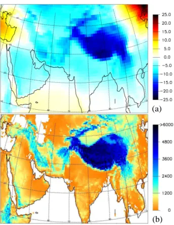
(a)
(b)
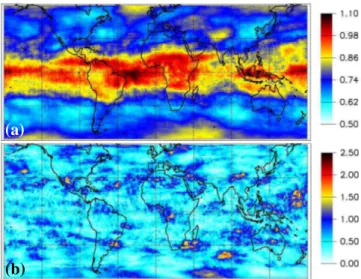
Fig. 8. (a) The difference between the average TO level (over the whole record) for a given grid point and the zonal average for the given latitude (in Dobson units). (b) Topographic map for the same region as in (a). Black colour indicates all the sites of elevation larger than 6000 m.
complicated spectral decomposition procedure by Vyushin et al. (2007) mentioned at the end of Sect. 2 might contain some uncertainties. For example, if the background trend is estimated by a picewise-linear trend, the choice of the break-ing point is somewhat arbitrary. Likewise, if the background trend is described by the EESC time series, there is no unique definition of EESC (Newman et al., 2007). Moreover, the calculated Hurst exponents are rather sensitively dependent on the frequency interval used for the parameter estimation.
Already the maps of spectral intensities in Fig. 4 indicate that TO variations are strongly affected by the atmospheric circulation. Of course, the obligate connection was recog-nised much earlier (see e.g., Dobson, 1968; Schoeberl, 1987; Salby and Callaghan, 1993). Clearly, the values of correla-tion exponents of TO are dominated by dynamical processes. Nonetheless, the fact that ozone abundances in recent years over the extrapolar regions of the Northern and Southern Hemisphere are 3% and 6% below pre-1980 values, respec-tively, is due to anthropogenic ozone depleting substances, that is due to chemistry (WMO, 2007). But this chemical
effect is apparently not strong enough to impact correlation exponents.
A particularly transparent linkage between the TO level and airflow dynamics is represented by the ozone “mini-holes”, which are spatially localised and transient ozone de-pletion events (McKenna et al., 1989; Peters et al., 1995).
Typical for the dynamics of mini-holes is a lifting of the tropopause above a tropospheric anticyclone and poleward motion of ozone poor subtropical air in the upper troposphere and lower stratosphere, which, in combination, causes a re-duction in column TO (Peters et al., 1995; Reid et al., 2000). The dynamics of mini-holes further results in equatorward excursions of polar air in the mid-stratosphere; in a situation when this air is chemically depleted by halogen chemistry in the polar vortex, particularly low ozone mini-holes may occur (Weber et al., 2002; Keil et al., 2007)
The mini-hole mechanism is demonstrated nicely by the visualisation of a “permanent” mini-hole over the Himalaya Mountains in Fig. 8a, where the difference between the aver-age total column ozone (computed over the whole period for a given gridpoint) and the zonal average determined along each degree latitude is plotted in a colour scale. (The topo-graphic setting for the same area is shown in in Fig. 8b.)
The strong coupling between measured TO and circula-tion patterns is evident (Fusco and Salby, 1999), however the general view assumes a restricted temporal range for correla-tions. The results in Fig. 7a suggest that the source of long-range correlations is in the dynamics of atmospheric circula-tion for both TO and temperature. It is well known that high-frequency atmospheric processes are crucial in achieving the long-term balance of energy, momentum, and water vapour in the atmosphere (Tsonis et al., 1999). Long-range tempo-ral correlations in the fluctuations mean that an anomaly of a given sign persists much longer (in statistical sense) than the characteristic timescales of the physical processes deter-mining the variability of the meteorological parameter. This behaviour is expected when the atmospheric flow is strongly coupled to the slowly varying components of the climate sys-tem such as the oceanic gyre modes. For example, a slowly changing sea surface temperature forcing can affect atmo-spheric flow for decades (Latif and Barnett, 1996).
Ozone and temperature share a number of common fea-tures. For example, the main source of “production” is around the equator, but both ozone and temperature are “gen-erated” over large extratropical areas with decreasing intensi-ties. Both ozone and heat are transported toward the poles by the atmospheric flow, mostly cyclones in the troposphere and by the Brewer-Dobson circulation in the stratosphere (Plumb and Eluszkiewicz, 1999). The curves in Fig. 7a are very similar, the smooth meridional changes of average correla-tion exponents are rather impressive. This observacorrela-tion fits to our present understanding of atmospheric dynamics, namely that the tropospheric and stratospheric processes are more strongly coupled than was believed earlier (Haynes, 2005).
Acknowledgements. This work was partly supported by the
Hun-garian Science Foundation (OTKA) under Grant No. T047233. IMJ thanks for a J´anos Bolyai Research Scholarship of the Hungarian Academy of Sciences.
Edited by: A. Tsonis
Reviewed by: one anonymous referee
References
Bartos, I. and J´anosi, I. M.: Nonlinear correlations of daily tempera-ture records over land, Nonlin. Processes Geophys., 13, 571–576, 2006,
http://www.nonlin-processes-geophys.net/13/571/2006/. Blender, R. and Fraedrich, K.: Long time memory in
global warming simulations, Geophys. Res. Lett., 30, 1769, doi:10.1029/2003GL017666, 2003.
Calisesi, Y. and Matthes, K., The middle atmospheric ozone re-sponse to the 11-year solar cycle, Space Sci. Rev., 125, 273–286, 2006.
Chen, Z., Ivanov, P. C., Hu, K., and Stanley, H. E., Effect of non-stationarities on detrended fluctuation analysis, Phys. Rev. E, 65, 041107, 2002.
Dobson, G. M. B.: Forty years’ research on atmospheric ozone at Oxford: a history, Appl. Opt., 7(3), 387–405, 1968.
Eichner, J. F., Koscielny-Bunde, E., Bunde, A., Havlin, S., and Schellnhuber, H.-J.: Power-law persistence and trends in the at-mosphere: A detailed study of long temperature records, Phys. Rev. E, 68, 046133, 2003.
Eyring, V., Butchart, N., Waugh, D. W., Akiyoshi, H., Austin, J., Bekki, S., Bodeker, G. E., Boville, B. A., Br¨uhl, C., Chipper-field, M. P., Cordero, E., Dameris, M., Deushi, M., Fioletov, V. E., Frith, S. M., Garcia, R. R., Gettelman, A., Giorgetta, M. A., Grewe, V., Jourdain, L., Kinnison, D. E., Mancini, E., Manzini, E., Marchand, M., Marsh, D. R., Nagashima, T., Nielsen, E., Newman, P. A., Pawson, S., Pitari, G., Plummer, D. A., Rozanov, E., Schraner, M., Shepherd, T. G., Shibata, K., Stolarski, R. S., Struthers, H., Tian, W., and Yoshiki, M.: Assessment of tem-perature, trace species and ozone in chemistry-climate simula-tions of the recent past, J. Geophys. Res., 111(D22), D22308, doi: 10.1029/2006JD007327, 2006.
Fusco, A. C. and Salby, M. L.: Interannual variations of total ozone and their relationship to variations of planetary wave activity, J. Climate, 12, 1619–1629, 1999.
Fraedrich, K.: Predictability: short- and long-term memory of the atmosphere, in: Chaos in Geophysical Flows, edited by: Bof-fetta, G., Larcotta, S., Visconti, G., and Vulpiani, A., Otto Edi-tore, Torino, 63–104, 2003.
Fraedrich, K. and Blender, R.: Scaling of atmosphere and ocean temperature correlations in observations and climate models, Phys. Rev. Lett., 90, 108501, 2003.
Fraedrich, K., Luksch, U., and Blender, R. A.: 1/f-model for long time memory of the ocean surface temperature, Phys. Rev. E, 70, 037301, 2003.
Govindan, R. B., Bunde, A., and Havlin, S.: Volatility in atmo-spheric temperature variability, Physica A, 318, 529–536, 2003. Haynes, P. H.: Stratospheric dynamics, Ann. Rev. Fluid Mech., 37,
263–293, 2005.
Hegger, R., Kantz, H., and Schreiber, T.: Practical implemen-tation of nonlinear time series methods: The TISEAN pack-age, Chaos, The software package is publicly available at http: //www.mpipks-dresden.mpg.de/∼tisean, 9, 413–435, 1999.
Hood, L. L.: The solar cycle variation of total ozone: Dynamical forcing in the lower stratosphere, J. Geophys. Res. D, 102, 1355– 1370, 1997.
Huybers, P. and Curry, W.: Links between the annual, Mi-lankovitch, and continuum of temperature variability, Nature, 441, 329–332, 2006.
J´anosi, I. M. and M¨uller, R., Empirical mode decomposition and correlation properties of long daily ozone records, Phys. Rev. E, 71, 056126, 2005.
Kantelhardt, J. W., Koscielny-Bunde, E., Rego, H. H. A., Havlin, S., and Bunde, A.: Detecting long-range correlations with detrended fluctuation analysis, Physica A, 295, 441–454, 2001.
Keil, M., Jackson, D. R., and Hort, M. C.: The January 2006 low ozone event over the UK, Atmos. Chem. Phys., 7, 961–972, 2007.
Kir´aly, A., Bartos, I., and J´anosi, I.M.: Correlation properties of daily temperature anomalies over land, Tellus A, 58, 593–600, 2006.
Kir´aly, A., and J´anosi, I.M.: Stochastic modeling of daily tempera-ture fluctuations, Phys. Rev. E, 65, 0511021, 2002.
Kir´aly, A. and J´anosi, I.M.: Detrended fluctuation analysis of daily temperature records: Geographic dependence over Australia, Met. Atmos. Phys., 88, 119–128, 2005.
Koscielny-Bunde, E., Bunde, A., Havlin, S., Roman, H. E., Goldre-ich, Y., and Schellnhuber, H. J.: Indication of a universal persis-tence law governing atmospheric variability, Phys. Rev. Lett., 81, 729–732, 1998.
Latif, M. and Barnett, T. P.: Decadal climate variability over the North Pacific and North America: Dynamics and predictability, J. Climate, 9, 2407–2423, 1996.
McKenna, D. S., Jones, R. L., Austin, J., Browell, E. V., Mc-Cormick, M. P., Krueger, A. J., and Tuck, A. F.: Diagnostic Stud-ies of the Antarctic Vortex During the 1987 Airborne Antarc-tic Ozone Experiment: Ozone Miniholes, J. Geophys. Res., 94, 11 641–11 668, 1989.
Monetti, R. A., Havlin, S., and Bunde, A.: Long term persistence in the sea surface temperature fluctuations, Physica A, 320, 581– 589, 2003.
Newman, P. A., Daniel, J. S., Waugh, D. W., and Nash, E. R.: A new formulation of equivalent effective stratospheric chlorine (EESC), Atmos. Chem. Phys. Discuss., 7, 3963–4000, 2007, http://www.atmos-chem-phys-discuss.net/7/3963/2007/. Patra, P. K., Santhanam, M. S., Manimaran, P., Takigawa, M., and
Nakazawa, T.: 1/f noise and multifractality in atmospheric-CO2 records, arXiv:nlin/0610038v1, 2006.
Pattanty´us- ´Abrah´am, M., Kir´aly, A., and J´anosi, I. M.: Nonuniver-sal atmospheric persistence: different scaling of daily minimum and maximum temperatures, Phys. Rev. E, 69, 021110, 2004. Pelletier, J. D.: Analysis and modeling of the natural variability of
climate, J. Climate, 10, 1331–1342, 1997.
Peng, C. K., Buldyrev, S. V., Havlin, S., Simons, M., Stanley, H. E., and Goldberger, A. L.: Mosaic organization of DNA nucleotides, Phys. Rev. E, 49, 1685–1689, 1994.
Peng, C. K., Havlin, S., Stanley, H. E., and Goldberger, A. L.: Quantification of scaling exponents and crossover phenomena in
442 P. Kiss, R. M¨uller and I. M. J´anosi: Long-range correlations of TOMS total ozone
nonstationary heartbeat time series, Chaos, 5, 82–87, 1995. Peters, D., Egger, J., and Entzian, G.: Dynamical aspects of ozone
mini-hole formation. Met. Atmos. Phys., 55, 205–214, 1995. Pilgram, B. and Kaplan, D. T.: A comparison of estimators for 1/f
noise, Physica D, 114, 108–122, 1998.
Plumb, R. A. and Eluszkiewicz, J.: The Brewer-Dobson circulation: dynamics of the tropical upwelling, J. Atmos. Sci., 56, 868–890, 1999.
Press, W. H., Teukolsky, S. A., Vetterling, W. T., and Flannery, B. P.: Numerical Recipes in C, Cambridge University Press, Cambridge, 1992.
Reid, S., Tuck, A., and Kiladis, G.: On the changing abundance of ozone minima at northern midlatitudes, J. Geophys. Res., 105(D10), 12 169–12 180, 2000.
Rybski, D., Bunde, A., Havlin, S., and von Storch, H.: Long-term persistence in climate and the detection problem, Geophys. Res. Lett., 33, L06718, doi:10.1029/2005GL025591, 2006.
Salby, M. L. and Callaghan, P. F.: Fluctuations of total ozone and their relationship to stratospheric air motions, J. Geophys. Res., 98, 2715–2727, 1993.
Schoeberl, M. R.: Dynamics of the middle atmosphere, Rev. Geo-phys., 25, 501–507, 1987.
Talkner, P. and Weber, R. O.: Power spectrum and detrended fluctu-ation analysis: Applicfluctu-ation to daily temperatures, Phys. Rev. E, 62, 150–160, 2000.
Toumi, R., Syroka, J., Barnes, C., and Lewis, P.: Robust non-Gaussian statistics and long-range correlation of total ozone, At-mos. Sci. Lett., 2, 94–103, 2001.
Tsonis, A. A., Roebber, P. J., and Elsner, J. B.: Long-range corre-lations in the extratropical atmospheric circulation: Origin and implications, J. Climate, 12, 1534–1541, 1999.
von Storch, H. and Zwiers, F.: Statistical Analysis in Climate Re-search, Cambridge University Press, Cambridge, 1999. Vyushin, D. I., Fioletov, V. E., and Shepherd, T. G.: Impact of
long-range correlations on trend detection in total ozone, J. Geo-phys. Res., 112, D14307, doi:10.1029/2006JD008186, 2007. Weatherhead, E. C. and Andersen, S. B.: The search for signs of
recovery of the ozone layer, Nature, 441, 39–45, 2006.
Weber, R. O. and Talkner, P.: Spectra and correlations of climate data from days to decades, J. Geophys. Res. D, 106, 20 131– 20 144, 2001.
Weber, M., Eichmann, K.-U., Bramstedt, K., Hild, L., Richter, A., Burrows, J. P., and M¨uller, R.: The cold Arctic winter 1995/96 as observed by GOME and HALOE: Tropospheric wave activity and chemical ozone loss, Q. J. R. Meteorol. Soc., 128, 1293– 1319, 2002.
WMO: Scientific assessment of ozone depletion: 2006, Global Ozone Research and Monitoring Project-Report No. 50, Geneva, Switzerland, 2007.