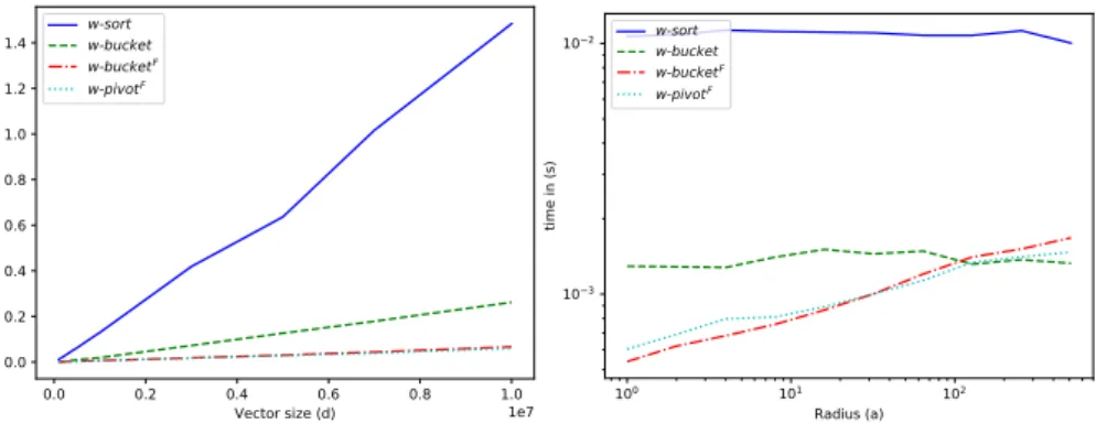
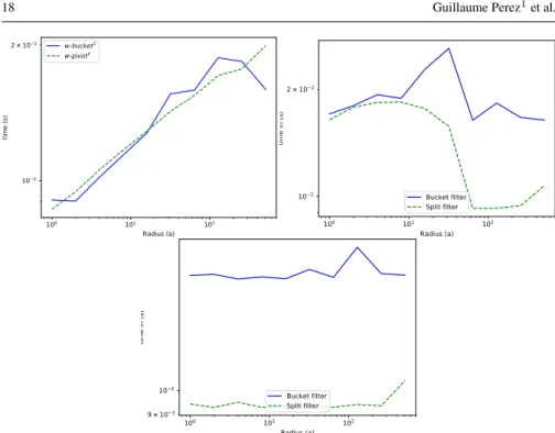
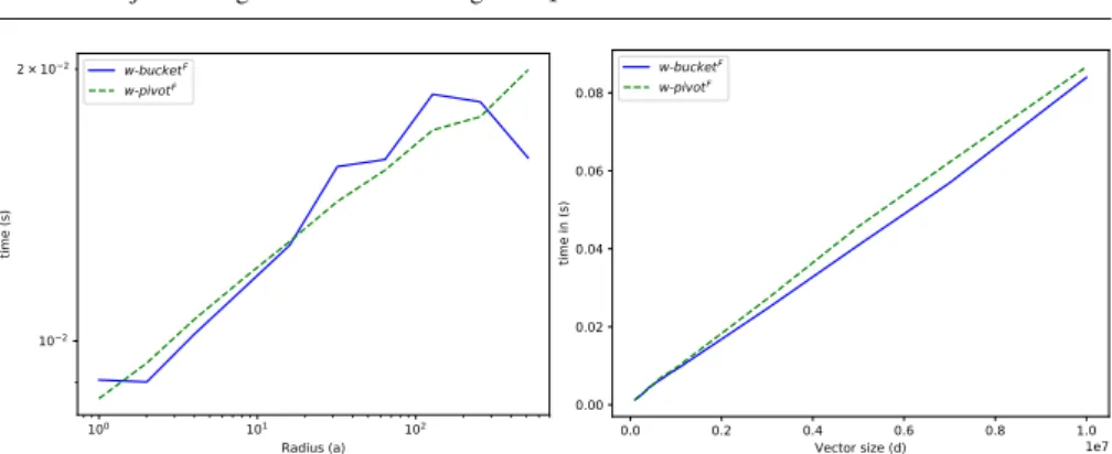
Efficient Projection Algorithms onto the Weighted 1 Ball
Texte intégral
Figure

Documents relatifs
It has been shown using a simple model of heat actuator that the quasi-static structural enrichment of the thermal modes can significantly improves the fidelity of the reduced
Key Words: Zeros of Entire Functions, Exponential Polynomials, Almost- Periodic Functions, Partial Sums of the Riemann Zeta Function..
• Algorithms in the cosparse analysis framework are de- fined in Section 2 in the spirit of Iterative Hard Thresh- olding (IHT, [2]) and Hard Thresholding Pursuit (HTP, [7]).. Note
In this article we have proposed a parallel implementation of the Simplex method for solving linear programming problems on CPU-GPU system with CUDA. The parallel implementation
Notes: The graphs represent odds ratios for each category on the probability of a leader having a positive and significant effect on the dependent variable as estimated
Keywords: large berth allocation problem, long term horizon, algorithm portfolio, quality run-time trade-off, real traffic
With forward branching and depth first search, if the problem is decomposable and solution memorization memorizes optimal solutions, then solution memorization dominates both
