The passive drinking effect: Evidence from Italy

HAL Id: halshs-00586686

https://halshs.archives-ouvertes.fr/halshs-00586686

Preprint submitted on 18 Apr 2011

HAL is a multi-disciplinary open access archive for the deposit and dissemination of sci-entific research documents, whether they are pub-lished or not. The documents may come from teaching and research institutions in France or abroad, or from public or private research centers.

L’archive ouverte pluridisciplinaire HAL, est destinée au dépôt et à la diffusion de documents scientifiques de niveau recherche, publiés ou non, émanant des établissements d’enseignement et de recherche français ou étrangers, des laboratoires publics ou privés.

The passive drinking effect: Evidence from Italy

Martina Menon, Federico Perali, Luca Piccoli

To cite this version:

Martina Menon, Federico Perali, Luca Piccoli. The passive drinking effect: Evidence from Italy. 2008. �halshs-00586686�

WORKING PAPER N° 2008 - 33

The passive drinking effect:

Evidence from Italy

Martina Menon

Federico Perali

Luca Piccoli

JEL Codes: C31, C34, C51, D12, D13

Keywords: collective model, demand system, sharing

rule, alcohol consumption, intra-household resources

distribution, policy implications

P

-

S

E

L

’E

A

-

48,BD JOURDAN –E.N.S.–75014PARIS TÉL. :33(0)143136300 – FAX :33(0)143136310

www.pse.ens.fr

CENTRE NATIONAL DE LA RECHERCHE SCIENTIFIQUE –ÉCOLE DES HAUTES ÉTUDES EN SCIENCES SOCIALES

The Passive Drinking Effect: Evidence from Italy

Martina Menon

Federico Perali

Luca Piccoli

June 26, 2008

Abstract

This paper investigates whether consumption of alcoholic beverages affects distribu-tion of resources among household members. We refer to this effect as passive drinking effect, highlighting the negative impact that alcohol addicted individuals can have on other household members’ wellbeing. To investigate this issue we rely on the collective framework and estimate a structural collective demand system. Our results show that for Italian households a high level of alcohol consumption influences the allocation of resources in favour of the husband, with a larger effect in poor households. This evidence implies that alcohol consumption is not only an individual problem. Public costs that are transferred to the other household members should be taken into account when designing social policies.

JEL Classification Codes: C31,C34,C51,D12,D13.

Keywords: collective model, demand system, sharing rule, alcohol consumption, intra-household resources distribution, policy implications.

Acknowledgements. We thank the Department of Economics of University of Verona, Paris School of Economics, the Institute of Health Management and Health Economics (Uni-versity of Oslo) and Statistics Norway for their support. Whe also thanks participants of the Workshop on Health Economics (held in Oslo) and Spring Meeting of Young Economic-sts (held in Lille) for their useful comments and suggestions; Special thanks goes to Rolf Aaberge, Francesco Avvisati, Sara Borelli, Eve Caroli, Andrew Clark, Sergio De Stefanis, Shoshana Grossbard, Snorre Kverndokk, Eugenio Peluso, Knut R. Wangen, Luca Zarri for their insightful comments and help. All errors are our own.

∗_{University of Verona} †_{Paris School of Economics}

This work is part of the ReAct project.1 ReAct is a research group based on voluntary work.

1

Introduction

This paper addresses the issue of whether a high level of individual alcohol consumption2 leads to negative economic consequences for other members of the household. The analogy with passive smoking is direct, but the transmission mechanism of the passive effect is less evident. It depends both on the behaviour of the drinker and the reduced amount of available resources.

In general, the analysis of consumption of addictive substances should be conducted through an intertemporal framework at the individual level. In fact, the process leading to addiction is strictly private and depends on the quantities consumed by the person itself in the past (Becker and Murphy, 1988; Epstein and Shi, 1993; Gruber and Köszegi, 2001). This is also related to the fact of considering alcohol as a bad rather than a good. A person may enjoy moderate drinking without suffering any side effect, while heavy drinkers may suffer diseases and several other problems. Therefore, for heavy drinkers it is not clear whether alcohol consumption generates utility, disutility or a mixture of both. In extreme cases, the individual may choose to drink because the disutility of not drinking is higher than the disutility of drinking.

So, from an individualistic point of view the household is often escluded from the analysis, playing at most a secondary role and considered simply as part of the environment in which the individual develops addiction. On the other hand, focussing the analysis on the household, the other members (non-heavy-drinkers) may suffer both a modified behavior of the drinker and the reduced resources available for them. In both cases, alcohol is a bad for them, not a good, and significantly affects the overall household welfare. In the present work we aim at giving the household the central role that it deserves as a potential victim of a social injustice. For instance, the old times English “egoistic” husband on Friday evening used to drink his wage at the pub, bringing no bread to the wife and the children (Seccombe, 1995). A similar example is given in Borelli and Perali (2002) for households of Djibouti, where husbands spend much of their wage on a legal drug, the qat, depriving other members of basic needs. As suggested by these examples, intra-household distribution of resources is a relevant determinant of a household’s welfare. Several negative “household internalities” caused by alcohol consumption, such as episodes of violence, misunderstandings, lack of attention, health problems, increased probability of car crashes, and so on, also suggest the need of a policy intervention. However, while these negative consequences are difficult to measure and evaluate economically, the intra-household distribution of resources is a reliable way to measure the negative impact that alcohol consumption can have on household welfare. The analytical tool that we adopt to study this issue is the collective framework of Chiappori (1988).

The adopted estimation strategy is similar to the one proposed by Browning, Bour-guignon, Chiappori, and Lechene (1994), where the estimation of a collective consumption models is performed.3 We test, through the estimation of a structural collective demand system, whether a high level of alcohol consumption induces a modification of the “sharing

1

ReAct(Research Group on Addiction) - http://dse.univr.it/addiction

2_{In the paper we will refer to consumption of goods and expenditures interchangeably. In the data, however,} we only observe good expenditures and not consumed quantities.

3_{Cherchye, de Rock, and Vermeulen (2008) also estimate a collective consumption model, but for the}

identification of the sharing rule they rely on a different set of assumptions, which makes our study not directly comparable to their work.

rule” with respect to households in which alcohol is not consumed. For instance, in some households, a despotic heavy drinker may take decisions regardless of other member’s needs. This situation may occur when a strong habit of alcohol consumption is present and a part of household resources is devoted to the daily measure of alcohol, and hence not available for other members. In these cases a policy intervention, aimed at restoring a more egalitarian intra-household distribution of resources, obtained reducing consumption of the vicious good and/or through gender specific policies, may be auspicable.

To our knowledge, in the literature there are no previous empirical studies on the link between alcohol consumption and the intra-household distribution of resources. Though we cannot compare our results with previous works, our findings are meaningful. According to our estimates, alcohol consumption significantly affects the intra-household distribution of resources which is biased towards the husband, especially for low income households. The results of this work seem to suggest that on average men tend to be more inclined to over-bearing behaviors when alcohol is consumed. Moreover, since from our estimation alcoholic beverages have a small own-price elasticity, a policy intervention of increased taxation on alcoholics may have a poor impact on consumption. Therefore, a policy intervention to in-crease the bargaining power of the wife within the household may result more effective in curbing male alcohol consumption.

The paper is organized as follows. Section 2 introduces the theoretical framework of Collective Choice Models and the demand system specification. Section 3 deals with the econometric method which will be applied. Section 4 describes the data used, Section 5 shows the results and Section 6 concludes.

2

The Model of Collective Choice

The collective framework (Chiappori, 1988, 1992) extends the unitary framework by explicitly modelling the household as a collection of individuals. This is obtained by introducing a sharing rule governing the allocation of resources among household members. Chiappori (1988, 1992) shows that for the identification of the sharing rule it is sufficient to observe the private consumption of at least one assignable good. This is as if the researcher were capable to observe the individual consumption, i.e. as if a household member was living alone. Browning, Chiappori, and Lewbel (2007) exploit this analogy to recover the sharing rule when household data do not record the private consumption of assignable goods. They estimate first the preferences of singles and then, assuming that an individual does not vary her preferences when changing marital status from single to married, the sharing rule. It should be noticed that this approach allows the recovery of the rule governing the allocation of resources across adult members of the household, but it is not possible to deduce the allocation rule between adults and children, because children never live alone.

Considering this limitation and that alcohol consumption of a young person living alone is structurally different from the consumption of an adult person living in a household, we choose the estimation approach by Chiappori, Fortin, and Lacroix (2002) extended to consumption as formulated in the subsequent section.

2.1

Theoretical Framework

In general, unitary models maximize a household utility function, which depends on consumed quantities of market goods, subject to a budget constraint. Consumption of single individuals within the household is not modeled and income pooling is assumed, that is individual incomes are put together to finance household expenditures and the final outcome is not affected by who has control over economic resources in the family. Within the collective theory the

decision taker is not the household as a whole but its members individually. This allows to have a representation of the household in which each member has its own preferences. In this context, it is possible to explain the intra-household distribution of resources through a function called sharing rule.

Assume that the household is composed by two members, the husband (m) and the wife (f ). In principle, each of them can receive a labour income, which, together with any non-labour income, contributes to the household income yh. Then the spouses, through a

bargaining process, decide how to divide the household income into the two quantities φ_m and φ_f,4 which represent the sharing rule.

Each member of the household may consume part of the goods purchased for the household oh at prices po or consume some exclusive goods ek, with k = m, f whose prices are pk.5

The exclusive goods may be male and female clothing,6 which are consumed by the husband and the wife exclusively.

The individual k maximizes his utility Uk accordins to the following program

max_ek_,okUk(ek, ok; θ_k) (1)

s.t. p0_kek+ p0_ook _{≤ φk} ek, ok_{≥ 0}

k = m, f ;

which leads to the following Marshallian demand functions xk_j = xk_j(φ_k, pk, po; θk), where xkj

is the demand of the k − th household member for good j, and j can be any good in ek or ok.

In principle we could estimate these demand functions separately, but in practice this is not feasible, since microeconomic datasets are collected at the household level. Moreover, even if individual expenditure is collected, it is difficult to assign an individual consumption to each good, since some goods are for their own nature public goods, while others, such as food, are in any case shared with all household’s member.

On the other hand, several datasets collect information on individual expenditure for some goods only, which is still a sufficient condition to identify the sharing rule (Bourguignon, 1999). This suggests that it is possible to construct a household demand system which takes into account for individual income effects (thanks to the sharing rule) and to recover at least some of the individual preferences parameters.

Considering that the household consumption vector x and the price vector p are

x= ⎡ ⎣ em ef om+ of ⎤ ⎦ and p = ⎡ ⎣ pm pf po ⎤ ⎦ ,

the household demand system can be specified by adding up individual demands, so that

xj(φm, φf, pm, pf, po; θm, θf) = xmj (φm, pm, po; θm) + xf_j(φf, pf, po; θf). (2)

We can now define the demand system specification, which will be used in the empirical exercise.

4_{Note that, being φ}

mand φf quantities, not relative measures, they are chosen such that φm+ φf = yh. 5_{In this study, we do not take into account public household goods, as housing, travelling costs and so on.} The reason is that the inclusion of such goods implies further complications which could cause identification issues for the sharing rule. See Browning, Chiappori, and Lewbel (2007) for a detailed discussion.

6_{In the literature, the most used exclusive good is leisure, which can provide the needed information for} the indentification of the sharing rule within a labour supply model.

3

Empirical Strategy

3.1

The Collective Quadratic Almost Ideal Demand System

The chosen demand system is an extension to the Almost Ideal Demand System originally proposed by Deaton and Muellbauer (1980). The model is extended with the introduction of a quadratic income term, following Banks, Blundell, and Lewbel (1997).7 Demographic characteristics interact multiplicatively with income in a theoretically plausible way (Barten, 1964; Gorman, 1976; Lewbel, 1985). The model is called “collective” because it incorporates the sharing rule through individual incomes for the two members of the household.

The following equation shows the budget share equation of the demand function for good i according to the specification of the collective quadratic almost ideal demand system (CQAIDS) derived in Appendix B

wi = αi+ ti(d) + X jγjiln pj+ β m i (ln φ∗m− ln a(p)) (3) + λ m i bm_(p)(ln φ∗m− ln a(p)) 2_{+ β}f i ¡ ln φ∗_{f − ln a(p)}¢+ λ f i bf_(p) ¡ ln φ∗_{f − ln a(p)}¢2,

where wi is the household budget share of good i, αi, γij, βi and λi are parameters, pj is

the price of good j, φ∗_m and φ∗_f are scaled individual expenditures determined by the sharing rule, a(p) and b(p) are two price indexes, t(d) is a translating function and d is a vector of demographic variables or household characteristics. The individual scaled total expenditures are defined as ln φ∗_m= ln φ_m(pm, pf, yh, z) − X iti(d) ln pi, (4) ln φ∗_f = ln φ_f(pm, pf, yh, z) − X iti(d) ln pi,

where φ_{m(·) and φf(·) are function of the household expenditure y}h, prices of the exclusive

goods pm and pf, and a vector of exogenous variables called distribution factors z, and pi is

price of good i.8

In order to comply with homogeneity properties of the demand system, the demographic specification of the budget share demand system is subject to a number of restrictions on the parameters. In particular, the following restrictions must hold

X iαi= 1; X iβi= 0; X iλi = 0; X iγij = 0; X jγij = 0; γij = γji; X iτir= 0.

This specification is consistent with the collective model stated in the previous section (equation 2) and allows to estimate individual income parameters βm_i , βf_i, λm_i and λf_i. Yet, it is not possible to estimate individual parameters for αi, γji and the parameters of the scaling

function ti(d), which are then estimated at the household level.

In the following section we discuss the identification of the sharing rule.

3.2

Specification of the Sharing Rule

In the specification of the CQAIDS described by equations (3) and (4), φ_{m(·) and φf(·) are} not observed variables: recovering the structure of the sharing rule is one of the objective of

7_{The choice is motivated in Appendix A, which provides evidence for a rank 3 demand system.}

8_{Distribution factors are exogenous variables that can affect the household behaviour only through their} impact on the decision process. In other words, the distribution factors do not affect either the individual preferences or the budget constraint. Examples of distribution factors used in empirical works are divorce ratio and sex ratio (Chiappori, Fortin, and Lacroix, 2002), wealth at marriage (Contreras, Frankenberg, and Thomas, .1997), and benefits (Rubalcava and Thomas, 2000).

this paper. Since we specified the sharing rule as a generalized function of observed variables, what we need is a parametric specification that when included in the demand system would allow to identify its parameters (Goldberger, 1972). The main issue is to find a viable way to use information on individual expenditures on some goods, which are recorded in several household budget datasets.

If we observe expenditure on some goods which are exclusively consumed by one of the household members, or for which a certain percentage can be certainly assigned to one of them, than the expenditure on those goods can be considered as individual consumption, and hence part of ek, as specified in equation (1). The other ordinaire goods, which are neither exclusive nor assignable, belong to oh_{, which is assumed to be equally divided between the}

spouses, that is om= of = 1₂oh.

Given the observed individual expenditure as p0_mem + p0_o1₂oh and p0_fef + p0_o1₂oh, it is possible to construct an index ω ∈ [0, 1] which determines the observed share of husband expenditure on total household expenditure

ωm =

p0_mem+ p0 o12oh

yh

. (5)

This implicitly defines the wife share of household expenditure as ωf = 1 − ωm and can

be used to define the individual expenditures yk as a function of household expenditure yh

as yk= ωkyh.

In the present work, to econometrically identify the sharing rule9 _{we use a technique}

borrowed from Pollak and Wales (1981) and Lewbel (1985), commonly used to incorporate demographic variables or exogenous factors into the demand functions, and from Bollino, Perali, and Rossi (2000), applied to estimate household technologies. In general, the idea is that demographic variables interact with exogenous prices or income and that their effect can be identified provided that sufficient variability is observed in the data.

Following this strategy, we define an income scaling function mk(pm, pf, z) a la Barten

(Barten, 1964; Perali, 2003), which relates the sharing rule φ_k(pm, pf, yh, z) to the observed

individual expenditure yk according to

φ_k(pm, pf, yh, z) = ykmk(pm, pf, z), for k = m, f. (6)

The estimation problem is similar to that of estimating a regression containing unobserv-able independent variunobserv-ables (Goldberger, 1972).

With the CQAIDS in the budget share form, we express equation (6) in natural logarithm, obtaining

ln φ_m(pm, pf, yh, z) = ln ym+ ln mm(pm, pf, z) (7)

ln φ_m(pm, pf, yh, z) = ln yf + ln mf(pm, pf, z),

where mm(pm, pf, z) and mf(pm, pf, z) are the scaling functions of individual income yk.

The identifying assumption in the model is that the portion of income of each member, ln ym and ln yf, can be recovered from observed expenditures on exclusive or assignable

goods. Namely, we define ln ym = ωmln yh and ln yf = (1 − ωm) ln yh, which implies that

ln ym+ ln yf = ln yh. Note that with respect to this definition of the individual expenditures,

the sharing rule should be considered a function determining the portion of the natural logarithm of income assigned as well, such that ln φ_{m(·) + ln φf(·) = ln y}h.

9_{Recall that the minimal information required for the identification of the sharing rule is the observability} of at least one assignable good, or, equivalently, two exclusive goods (Bourguignon, 1999). If a good is exclusive, and there are no externalities, for a given observed demand x(p, y) satisfying the Collective Slutsky property (Chiappori, 1988, 1992; Chiappori and Ekeland, 2002, 2006), and such that the Jacobian Dpx(p, y) is invertible, then the sharing rule is identified.

The definitions of the sharing rule expressed in equation (7) and the fact thatX

kln φm =

ln yh are a key feature for the identification of the sharing rule. They imply that the following

condition must hold

ln mm(pm, pf, z) = − ln mf(pm, pf, z), (8)

which allows us to set ln mm(·) = ln m(·) and ln mf(·) = − ln m(·). In this way, only one set

of additional parameters belonging to the income scaling function m(·) needs to be estimated, identifying the sharing rule for both household members.

Given equations (7) and (8), it is possible to rewrite equations (4) as

ln φ∗_m= ωmln yh+ ln m(pm, pf, z) − X iti(d) ln pi ln φ∗_{f = (1 − ω}m) ln yh− ln m(pm, pf, z) − X iti(d) ln pi.

In analogy to function ti(d), function m(pm, pf, z) is identified provided there is enough

variation in the individual prices pm and pf and in the distribution factors z.10

In our empirical study, we specify m(pm, pf, z) as a Cobb-Douglas function, so that the

logarithmic specification is linear in the parameters

ln m(pm, pf, z) = φ0ln pr+

XN

n=1φnln zn,

where pr is a price ratio, whose specification is given below, and N is the dimension of

vector z. With this specification there is an additional restriction, which is that distribution factors z must differ from the demographic variables d. If it were not so, the parameters ln m(pm, pf, z) and ti(d) would not be identified for the variables that are shared by z and

d.

In the next section we specify the econometric strategy used to perform our estimates.

3.3

Zero Expenditure

Econometricians working with household micro-data often are faced to the zero expenditures problem, especially when working with disaggregate goods, which is the case, for example, of alcohol consumption, tobacco or clothing. Since coefficient estimates are inconsistent when only observed positive purchase data are used, the proper correction technique has to be used.

The econometric methods dealing with the zero expenditure issue differ for the assump-tions related to the source of zero expenditures. For example, the Tobit model (Amemiya, 1985; Maddala, 1983) captures the corner solutions for the utility maximization problem, which implies that the observation is zero just because the household decided not to consume on the basis of disposable income, prices and preferences. This could be the case for some goods, such as semi-durables, which may not be purchased in the reference period because they give utility for more than one period and a household may need to buy them only few times in a year. This situation is called infrequency of purchases.

On the other side, the Double-Hurdle model (Yen, 1993) assumes that zero expenditures are explained by a decision process that arises from unobserved latent variables which drive consumer choices. The model allows a separate estimation of participation and expenditure parameters. This is the case of alcohol, which may not be consumed because of moral conviction or health problems, which may not be observable in the survey. However, this model is not useful when considering semi-durable goods.

1 0

The proof is similar to proving that function ti(d)is identified, as shown in Gorman (1976), Lewbel (1985) or Perali (2003).

An alternative to the Double-Hurdle model is the Heckman two-step estimator, which assumes that zero expenditures are due to sample selection bias (Heckman, 1979) and are treated as a mispecification error. This approach allows for separate estimates of participation and expenditure parameters.

In the original model, the first stage determines the participation probability using a probit regression, and then, in the second stage, Heckman proposes a specification for the omitted variable which can be used to correct the sample selection bias. The omitted variable is the inverse Mill’s ratio, which is the ratio between density and cumulative probability function of the standard normal distribution.

In this paper we use a generalization of the Heckman two-step estimator overcoming the issues which emerge in Amemiya (1978, 1979) and Heien and Wessells (1990). In particular, we refer to the work of Shonkwiler and Yen (1999), which proposes a consistent, though still simple, two-step generalized Heckman estimator for a censored system of equations.

In choosing the proper estimator, we had to keep in mind that the dataset has zero expenditures for two goods: alcohol and education and recreation. The double-hurdle model is particularly well suited for alcohol consumption, which is what we are focussing on, but is not general enough to consider other sources of zero expenditures. Hence, we decided to use the generalized Heckman estimator, which is well suited for a rather large source of zero expenditures, is consistent with a two-stages decision process similar to that of the Double-Hurdle and keeps things simple.

Following Shonkwiler and Yen (1999) and Arias, Atella, Castagnini, and Perali (2003), consider the following general limited dependent variables system of equations11

y_it∗ = f (xit, θi) + it, d∗it= zit0 τi+ υit, (9) dit= ½ 1 if d∗ it > 0 0 if d∗_{it ≤ 0} yit = dity ∗ it, (i = 1, 2, ..., m; t = 1, 2, ..., T ),

where i represents the i-th equation and t the t-th observation, yit and dit are the observed

dependent variables, y_it∗ and d∗_it are the latent variables, xit and zit are vectors of exogenous

variables, θiand τi are parameters, and, it and υitare random errors. Without entering into

details, system (9) can be written as

yit= Ψ(zit0τi)f (xit, θi) + ηiψ(zit0 τi) + ξit,

where Ψ(·) and ψ(·) are univariate normal standard cumulative distribution and probability density functions respectively. The system can be estimated by means of a two-step proce-dure, where τi is estimated using a Maximum Likelihood probit estimator, and is used to

calculate Ψ(v_it0 τi) and ψ(v0itτi). Successively, estimates of θi and ηi in the system

yit= Ψ(zit0τˆi)f (xit, θi) + ηiψ(zit0 ˆτi) + ξit (10)

are obtained by Full Information Maximum Likelihood.

4

Data Description

The data used in this work is drawn from the Italian household expenditure survey (Con-sumi delle Famiglie Italiane) for the period 2002-2004. We selected households composed by married couples without dependent children with an observed positive consumption for

male and female clothing.12 To ensure a demographically homogeneous sample, we excluded households in which at least one member is retired from work. In this way we restrict our study to working couples with a similar lifestyle. The sample includes 1947 observations. The dataset information has been matched with individual alcohol consumption data from ISTAT 2002 survey on the standard of living (Indagine Multiscopo su Stili di Vita e Condizioni di Salute).13

In the latter dataset, information is collected on an individual basis. This feature allows us to assign alcohol consumption respectively to the husband or to the wife. Clothing can be exclusively assigned to the husband and the wife since male and female clothing is separately recorded in the expenditure survey.

We consider only expenditure of non durable goods, hence the aggregated expenditure categories considered are food, alcohol, clothing, education and recreation, and other goods. Household-specific prices are assigned following the procedure described below.

Since the ISTAT survey records only expenditure information, the lack of information about quantities purchased precludes the possibility to calculate household specific unit val-ues. On the other hand, ISTAT’s price indexes have an aggregation level similar to that of the survey, but are not sufficient to provide plausible elasticities. For this reason, we use a procedure, originally proposed by Lewbel (1989) and applied by Atella, Menon, and Perali (2003), to construct pseudo unit values.

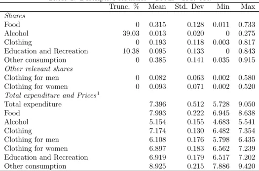
Table 1 and Table 2 report the descriptive statistics of the sample. The set of demo-graphic variables d includes macro regions (North-East, North-West and Center), a dummy variable to capture seasonality (particularly Christmas time), a dummy variable indicating if head households have a university or higher degree, a dummy variable to indicate that the household does not live in urban areas (rural), a dummy variable indicating that husband is an employee, a variable signaling if at least one in the couple smokes and two dummy variables to control for possible differences in the year of relevation. The exogenous variables chosen for the sharing rule are quite limited by the disposable information in the dataset and are defined as follows. Thus the distribution factors z are the price ratio (price-r) is the price of male clothing divided by the sum of male and female clothing prices, the age ratio (age-r) is defined as husband’s age divided by the sum of both members ages, and the education ratio (edu-r) is defined as husband’s years of schooling divided by the sum of both members years of schooling.

In the next section we present the results and comments.

5

Results

This section describes the results coming from the estimation of model (10) where yit and

f (xit, θi) are replaced by wit and the right hand side of equation (3), respectively.

The estimates of the parameters are obtained by Full Information Maximum Likelihood estimation of a collective Quadratic Almost Ideal Demand System, as described in Section 3.1. Zero observed expenditures are corrected applying the generalized Heckman two-step 1 2_{We restrict to positive clothing expenditures because this is the source of identification for the sharing} rule. Using observations with no clothing expenditure would not add useful information for the identification of the sharing rule.

1 3_{The imputation of the variable was conducted using a semi-parametric method.The technique works as}

follows. Both samples share a number of variables which describe household characteristics. Divide both samples in cells determined by the same household characteristics. To impute a variable, for each household in the cell randomly pick up a value from the corresponding cell in the second sample. This method has two particular advantages: first, zero observed expenditures are preserved, and second, the overall distribution of the variable remains almost unchanged after imputation.

estimator proposed by Shonkwiler and Yen (1999) as applied by Arias, Atella, Castagnini, and Perali (2003).

Symmetry and homogeneity properties of the demand system are ensured by construction, with the Slutsky matrix having two individual income terms which sum up to the household income effect.

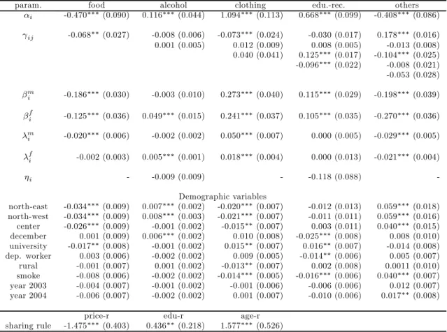
In Table 4 we present the estimates of the CQAIDS demand system. In general, income parameters (αi, βm, βf, λm, λf) are significant with the exception of alcohol income

pa-rameters, which are non significant for the husband, and teh quadratic temrs of education and recreation. The zero correction parameters η_i parameters are not significant, indicating that the observed zero expenditures should not bias parameter estimates. Among the demo-graphic variables, the general trend is towards small parameter values, even if many of them are significantly different from zero. The dummy variables included to control for the year of relevation of the data are generally not significant.

The alcohol demand equation is insensible to most demographic variables. A positive effect is observed if the household lives in the north of Italy. This is as expected and is cited in some ISTAT reports on alcohol consumption. The tendency is to relate different behavior to climate differences. In the south, a warmer temperature discourages consumption of alcoholic beverages in summer, while during winter rigid northern temperatures tend to favour consumption of spirits. A positive effect is also observed for the seasonality control variable. This is also as expected, since during winter holidays there is a strong increase in champagne wine demand.

More interestingly, the education parameter is found to be non significant to explain alcohol expenditure. In Italy it is common practice to drink a glass of wine at meals and a moderate consumption of good quality wine is an encouraged behavior, and this could explain the evidence. Hpwever, even if not signifincant, the parameter is negative, indicating that if there had been an effect it would have been as expected.

Contrary to what we expect, we find a non significant parameter for the smoke dummy variable. This should not be interpreted ad a negative evidence about the link between smoking and drinking since we should take into account that participation and consumption are treated separately. In the participation equation (see Table 5) the parameter is positive and strongly significant, indicating a possible gateway effect between alcohol and tobacco. The non significant parameter in the demand equation states that there is not a positive relation between expenditure on alcohol and the fact of being a smoker. In other words, a smoker has a higher probability of being a drinker, but smoking does not influence how much one drinks.

The parameters of the sharing rule tell us that the husband’s share of total expenditure is negatively influenced by the price of male clothing. If the husband is more educated than his wife, the effect will be of an increase in its share of household resources, and the same happens if the husband is older than the wife. These parameters are all significant.

Table 6 shows (double-sided numerical) income elasticities, compensated price elasticities and standard deviations derived via delta method. Own-price elasticities are consistent with consumption theory. According to their size, education and recreation is the most elastic good to price and income changes, while alcohol is one of the less elastic. Alcohol own-price elasticity is the smallest of the group of goods, suggesting that a policy of an increased taxa-tion on alcoholic beverages may not have much success in reducing consumptaxa-tion.14 Therefore, in cases of price variations, it is plausible that individuals substitute other goods for alcohol. Education and recreation has by far the most variable elasticities, suggesting that within this group of goods it may be used as a buffer for income or price shocks.

1 4

It could be argued, however, that the increased taxation may serve to compensate for the negative social effects produced by alcohol abuse.

.4 .5 .6 .7 .8 Sharing Rule 6 6.5 7 7.5 8 8.5 Ln of Total Expenditure

Scatter Plot Strong Drinkers

Abstemious

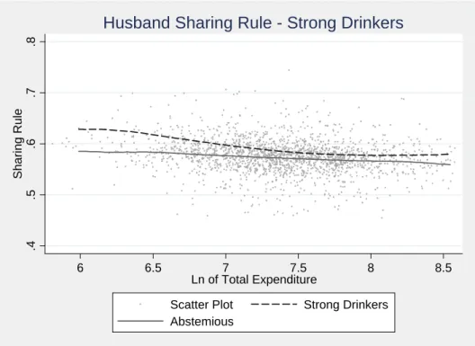
Husband Sharing Rule - Strong Drinkers

Figure 1: Heavy drinkers

.4 .5 .6 .7 .8 Sharing Rule 6 6.5 7 7.5 8 8.5 Ln of Total Expenditure

Scatter Plot Husband main drinker

Wife main drinker Abstemious

Husband Sharing Rule - Main Drinker

Other elasticities are as expected and in line with usual findings in the literature. To detail further the intra-household income distribution analysis, we have depicted fig-ures 1 through 4, which represent the relative husband sharing rule, expressed as the ratio be-tween husband expenditure and total household expenditure (ln φm_{(·)/ ln y}h). These pictures are drawn by means of nonparametric regressions of the sharing rule by total expenditure, selecting groups of households with some characteristics of interest.

In Figure 1, we select a group of abstemious households and a group of heavy15alcohol con-sumers. The sharing rule is different in these groups, with the husband being favoured in the distribution of resources when alcohol consumption is large, especially for low income house-holds. A t-test performed on the average sharing rules for strong drinkers and abstemious confirms that there is a positive difference with a confidence level of 99%.16 According to this analysis, alcohol consumption seems to cause a household income distribution modification with respect to abstemious households which could motivate a policy intervention.

In Figure 2 we further investigate the relation between alcohol consumption and the shar-ing rule. Selectshar-ing households by its main drinker,17 the sharing rule shifts towards the main drinker himself/herself, except for households with low total expenditure, where even when the main drinker is the wife, the sharing rule is still shifted towards the husband.18 When the main drinker is the man the effect is evident and could be explained by a combination of several factors. Among other causes, there could be the fact that men tend to have a overbearing behavior more frequently than women, and this tendency may be strengthened by alcohol, which makes them more self confident and violent. This could also explain why when the main drinker is the wife the distribution of resources still favours the husband when the household is poor.19 In these households there could be a despotic husband which tends to keep control on household resources and to impose his decisions. In such a situation, it may happen that the wife falls into depression and/or uses alcohol as a mean to “escape from that reality”.

The situation depicted by Figure 1 and 2 justifies a policy intervention. However, as stated above, a strategy based on direct taxation is likely to have a small impact. The problem is more serious for low income households and a price increase may even worsen their situation. Instead, we are in favour of gender specific policies with the aim of balancing the decisional power within the household. Just as an example, subsidies for poor households or children subsidies should be given to woman. In this way the wife gains bargaining power and there is less probability that the money is spent on alcohol both because she feels more self confident or because the husband has less money to spend on alcohol. This policy, which has been implemented with much success for micro-credit policies in developing countries, has no additional costs and could bring a noticeable welfare improvement to those households.

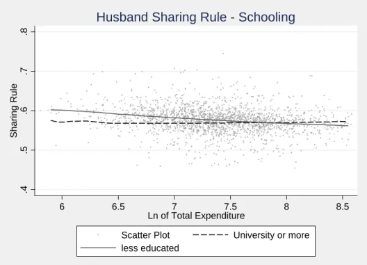
Figure 3 plots the sharing rule by the household head’s education. The picture shows that less education generates a distribution of resources in favour of the husband for middle and low income households, while for households with higher level of income the situation is unchanged. This seems to be in contrast with the positive sign of the edu-r parameter in the sharing rule, which indicates that the member with higher education will have a greater

1 5_{We consider heavy consumers households which have an alcohol budget share above 0.035.}

1 6

The abstemius sharing rule has an average value of 4.17 with a standard deviation of 0.38 over a subsample of 760 observations, while the strong drinker sharing rule has an average value of 4.30 with a standard deviation of 0.37 over a subsample of 175 observation. The test value is 4.08 with 933 degree of freedom, which largely rejects the null hypothesis of a difference equal to zero.

1 7_{The household member is the main consumer if he/she consumes at least 75% of household alcohol}

consumption.

1 8_{Remember that represented is always the husband sharing rule, hence, a higher line means that the}

husband is favoured, while a lower line means that the wife is favoured.

1 9_{In poor households there is a higher probability that the wife does not work and in psychology there is} evidence that housewives may feel subjugated and tend to drink more.

.4 .5 .6 .7 .8 Sharing Rule 6 6.5 7 7.5 8 8.5 Ln of Total Expenditure

Scatter Plot University or more

less educated

Husband Sharing Rule - Schooling

Figure 3: Schooling .4 .5 .6 .7 .8 Sharing Rule 6 6.5 7 7.5 8 8.5 Ln of Total Expenditure

Scatter Plot North

South Center

Husband Sharing Rule - Macro Regions

amount of household resources. However this is not a real contrast since the parameter only captures the relative education, and not the level itself.

Figure 4 shows that the sharing rule is scarcely influenced by macro-regional divisions. There is a difference for low income households, where South shows a distribution more in favour of the husband. Looking at parameters in Table 4 we see that macro regions have generally significant parameters, which means that consumption levels are different across macro regions, but that this difference does not always reflect much to the sharing rule.

The following section concludes and proposes future developments to this work.

6

Conclusions

In this paper we present some evidence that for Italian households an excessive alcohol consumption can affect the distribution of resources within the household. The results are relatively strong, even for a country which is supposed to have a relatively advanced social background.

When a significative amount of alcohol is consumed we find a systematic shift of the sharing rule towards the husband. This shift is greater for low income households, implying that the effects of alcohol consumption on the intra-household income distribution are heavier for low income households with a heavy drinker. This provides the rational for a policy intervention aimed to contrast this phenomenon. However, since the own-price elasticity of alcohol is the lowest across goods, we suggest that the proper policy should not be that of increasing direct taxation on alcoholic beverages, since the price increase would probably be shifted to other goods.20

Taking into account individual alcohol consumption, we find that the sharing rule shifts toward the main drinker in the household, but with a substantial difference between the husband and the wife. In fact, when the main drinker is the husband, the shift is evident in the whole range of household income distributions.21 When the main drinker is the wife the effect is less evident, and for poor households, even when the main drinker is the wife, the distribution of resources changes in favour of the husband. In this case the role of alcohol in behavioral terms is less evident, but still can be explained, for instance as an increased vulnerability of the drinker.

The generalized shift of resources toward the husband in the case of large alcohol con-sumption is the sum of these two effects. This means that the proper policy for the reduction of the modification of the distribution of resources observed in the case of alcohol consumption should be gender specific.

However, these issues need further investigations and we are planning future developments to extend the analysis in several ways. The first extension regards the quality of data available. We are building a new dataset to incorporate much more information on single household components lifestyle, health, income and labour supply. This will be done by matching three sources of data available in Italy in separate datasets provided by ISTAT and the Bank of Italy.22

Regarding the estimation technique, we are investigating whether it could be more con-venient to estimate the system by means of a Minimum Distance Estimator. This technique would be much useful in treating the observed zero expenditures. To this extent, we could

2 0

This is true only if we consider an aggregate alcohol good. If we are willing to differentiate taxation by the alcohol content of each beverage, as spirits, wine and beer, the response would probably be different, and an increase taxation of spirits would probably shift consumption towards wine and beer. However, due to our data, we cannot make this interesting analysis.

2 1

The shift is still larger for poor households.

2 2_{In this regard, the good results obtained by matching data on individual alcohol consumption incentives} us to proceed in this direction.

apply the proper zero correction technique to each good, allowing the use of specific correction techniques like Double-Hurdle, Infrequent Purchases, and so on.

An interesting development would regard the Pareto efficiency of household consumption choice. In our analysis, we do not explicitly take into account the possibility of inefficient resources allocation. However, the collective model would be a suitable instrument to answer this question since it allows an estimation of individual income effects. These income effects could be employed to test Pareto efficiency following the intuition of Browning, Bourguignon, Chiappori, and Lechene (1994) and Udry (1996).

In the present work, we focus our attention to the distribution of resources between husband and wife alone. We are working to extend the sharing rule in order to cover three members of the household simultaneously (husband, wife and children). The usefulness of such a specification is evident when evaluating the effects of alcohol abuse, in which the looser may be the children, the wife or both.

References

Amemiya, T. (1978): “On a Two-Step Estimationof a Multivariate Logit Model,” Journal of Econometrics, 8, 13—21.

(1979): “The Estimation of a Simultaneous Equation Tobit Model,” International Economic Review, 20(1), 169—81.

(1985): Advanced Econometrics. Harvard University Press, Cambridge, Massa-chusetts.

Arias, C., V. Atella, R. Castagnini, and F. Perali (2003): “Estimation of the Shar-ing Rule Between Adults and Children and Related Equivalence Scales Within a Collec-tive Consumption Framework,” in Household Behavior, Equivalence Scales, Welfare and Poverty, ed. by C. Dagum,and G. Ferrari. Physica-Verlag.

Atella, V., M. Menon, andF. Perali (2003): “Estimation of Unit Values in Cross Sec-tions Without Quantity Information,” in Household Welfare and Poverty, ed. by G. Ferrari,

and C. Dagum. Physica Verlag.

Atkinson, A. B., G. Gomulka,andN. H. Stern (1990): “Spending on Alcohol: Evidence from the Family Expenditure Survey 1970-1983,” Economic Journal, 100, 808—27.

Banks, J., R. Blundell,andA. Lewbel (1997): “Quadratic Engel Curves and Consumer Demand,” The Review of Economics and Statistics, 79(4), 527—39.

Barten, A. P. (1964): “Family Composition, Prices and Expenditure Patterns,” in Econo-metric Analysis for National Economic Planning: 16th Symposium of the Colston Society, ed. by P. Hart, G. Mills, and J. K. Whitaker. Butterworth.

Becker, G. S., and K. Murphy (1988): “A Theory of Rational Addiction,” Journal of Political Economy, 96, 675—700.

Bierens, H. J.,andH. A. Pott-Buter (1987): “Specification of Household Engel Curves by Nonparametric Regression,” Econometric Reviews, 9, 123—84.

Blundell, R., P. Pashardes, and G. Weber (1993): “What Do We Learn About Con-sumer Demand Patterns from Micro-Data?,” American Economic Review, 83, 570—97. Bollino, C. A., F. Perali, and N. Rossi (2000): “Linear Household Technologies,”

Journal of Applied Econometrics, 15(3), 275—87.

Borelli, S., and F. Perali (2002): “Drug Consumption and Intra-Household Distribu-tion of the Resources: The Case of Qat in an African Society,” in Household Behaviour, Equivalence Scales and Well-Being, ed. by Dagum, and Ferrari, Collana Physica Verlag. Springer.

Bourguignon, F. (1999): “The Cost of Children: May the Collective Approach to House-hold Behavior Help?,” Journal of Population Economics, 12, 503—21.

Browning, M., F. Bourguignon, P. A. Chiappori,andV. Lechene (1994): “Incomes and Outcomes: A Structural Model of Intrahousehold Allocation,” Journal of Political Economy, 102(6), 1067—96.

Browning, M., P. A. Chiappori, and A. Lewbel (2007): “Estimating Consumption Economies of Scale, Adult Equivalence Scales, and Household Bargaining Power,” forth-coming.

Cherchye, L., B. de Rock, and F. Vermeulen (2008): “Economic Well-Being and Poverty Among the Elderly: An Analysis Based on a Collective Consumption Model,” Discussion paper.

Chiappori, P. A. (1988): “Rational Household Labor Supply,” Econometrica, 56(1), 63—90.

(1992): “Collective Labor Supply and Welfare,” Journal of Political Economy, 100(3), 437—67.

Chiappori, P. A., and I. Ekeland (2002): “The Micro Economics of Group Behavior: Identification,” working paper, Department of Economics, University of Chicago.

(2006): “The Micro Economics of Group Behavior: General Characterization,” Journal of Economic Theory, 127(1), 1—26.

Chiappori, P. A., B. Fortin, and G. Lacroix (2002): “Marriage Market, Divorce Leg-islation, and Household Labor Supply,” Journal of Political Economy, 110(1), 37—72.

Contreras, D., E. Frankenberg, and D. Thomas (.1997): “Child Health and the Dis-tribution of Household Resources at Marriage,” Discussion paper, UCLA, Mimeo RAND.

Deaton, A. S.,andJ. Muellbauer (1980): “An Almost Ideal Demand System,” American Economic Review, 70, 321—26.

Epstein, L., and S. Shi (1993): “Habits and Time Preference,” International Economic Review, 34, 61—84.

Gill, L., and A. Lewbel (1992): “Testing the Rank of Estimated Matrices with Appli-cations to Factors, State Space, and ARMA Models,” Journal of the American Statistical Association, 87, 766—76.

Goldberger, A. S. (1972): “Maximum-Likelihood Estimation of Regressions Containing Unobservable Independent Variables,” International Economic Review, 13(1), 1—15.

Golub, G. H.,andC. F. VanLoan (1983): Matrix Computations. John Hopkins University Press, Baltimore.

Gorman, W. M. (1976): “Tricks with Utility Functions,” in Proceedings of the 1975 AUTE Conference, Essays in Economic Analysis, ed. by M. J. Artis,andA. R. Nobay. Cambridge University Press, Cambridge.

Gruber, J., and B. Köszegi (2001): “Is Addiction "rational"? Theory and Evidence,” The Quarterly Journal of Economics, 116(4), 1261—1303.

Härdle, W., and M. Jerison (1988): “The Evolution of Engel Curves over Time,” Dis-cussion Paper A-178, SFB 303, University of Bonn.

Hausman, J. A., W. K. Newey,andJ. L. Powell (1995): “Nonlinear Errors in Variables: Estimation of some Engel Curves,” Journal of Econometrics, 65, 205—33.

Heckman, J. (1979): “Sample Selection Bias as a Specification Error,” Econometrica, 47(1), 153—61.

Heien, D.,andC. R. Wessells (1990): “Demand Systems Estimation with Microdata: A Censored Regression Approach,” Journal of Business and Economic Statistics, 8, 365—71.

Hildebrand, W. (1994): Market Demand: Theory and Empirical Evidence. Princeton Uni-veristy Press, Princeton.

Leser, C. E. V. (1963): “Forms of Engel Functions,” Econometrica, 31, 694—703.

Lewbel, A. (1985): “A Unified Approach to Incorporating Demograpic or Other Effects Into Demand Systems,” Review of Economic Studies, 70, 1—18.

(1989): “Identification and Estimation of Equivalence Scales under Weak Separa-bility,” Review of Economic Studies, 56, 311—16.

(1991): “The Rank of Demand Systems: Theory and Nonparametric Estimation,” Econometrica, 59, 711—30.

(2002): “Rank, Separability, and Conditional Demand,” Canadian Journal of Eco-nomics, 35(2), 410—413.

Maddala, G. S. (1983): Limited-Dependent and Qualitative Variables in Econometrics. Cambridge University Press, Cambridge.

Pagan, A., and A. Ullah (1999): Nonparametric Econometrics. Cambridge University Press, London.

Perali, F. (2003): The Behavioral and Welfare Analysis of Consumption. The Cost of Children, Equity and Poverty in Colombia. Springer-Verlag.

Pollak, R., and T. J. Wales (1981): “Demographic Variables in Demand Analysis,” Econometrica, 49(6), 1533—51.

Rubalcava, L., and D. Thomas (2000): “Family Bargaining and Welfare,” Discussion Paper 00-10, RAND - Labor and Population Program.

Seccombe, W. (1995): Weathering the Storm. New York: Verso, London.

Shonkwiler, J. S., and S. T. Yen (1999): “Two-Step Estimation of a Censored System of Equations,” American Journal of Agricultural Economics, 81, 972—982.

Silverman, S., and B. W. Silverman (1986): Density Estimation for Statistics and Data Analysis. CRC Press.

Udry, C. (1996): “Gender, Agricultural Production and the Theory of the Household,” Journal of Political Economy, 104(5), 1010—46.

Working, H. (1943): “Statistical Law of Family Expenditure,” Journal of the American Statistical Association, 38, 43—56.

Yen, S. T. (1993): “Working Wives and Food Away from Home: The Box-Cox Double-Hurdle Model,” American Journal of Agricultural Economics, 75, 884—95.

Appendix A: Non-parametric Engel curves and Rank Test

Engel curves are a widely used tool to assess the relationship between consumption and income. They have been studied for a long time, but still there is no agreement on which functional form is best suited to describe this relationship. According to the early work of Working (1943) and Leser (1963) Engel curves could be considered linear in the log of income, but later studies, among which Atkinson, Gomulka, and Stern (1990), Bierens and Pott-Buter (1987), Blundell, Pashardes, and Weber (1993), Hausman, Newey, and Powell (1995), Härdle and Jerison (1988), Hildebrand (1994), and Lewbel (1991), have shown that this specification is rather poor in describing Engel curves for some goods. The general evidence on micro-data is in favour of a quadratic relationship between budget shares and the log of total expenditure,23 i.e. a rank 3 demand system.24

Even if there is some general agreement on the use of quadratic Engel curves, we provide nonparametric evidence to verify the rank of the demand system. We use single equation non-parametric Engel curve estimation,25 and model the budget share of each good to be a non-linear function of the natural logarithm of total expenditure. Following Banks, Blundell, and Lewbel (1997) and Perali (2003), we plot in Figure 5 non-parametric estimates of alcohol individual Engel curves (orange line) and its 95% confidence interval (blue dashed lines). Similarly in Figure 6 we plot clothing individual Engel curves. Figure 7 represents household level Engel curves for food, education and recreation and other goods. In each graph also a quadratic polynomial regression (purple line) is plotted. The purpose is to verify whether a quadratic relationship can fit within the Engel’s curves confidence intervals. Finally, along with Engel curves, we present nonparametric kernel bivariate density estimates and contour density plots.

A graphical analysis shows that the relation between food, alcohol for the wife, female clothing and total log expenditure can be represented by a linear functional form, while all other goods except male clothing exhibit a shape rather close to a quadratic function. However, considering the confidence interval, a quadratic form cannot be excluded for clothing either.

To deepen the analysis we perform a non-parametric rank test for the demand system (Gill and Lewbel, 1992). This test does not need the specification of a functional form for the demand system, and hence avoids specification errors. The test is based on the estimated pivots of a matrix associating shares to functions of the total expenditure. The data matrix is decomposed using the Lower-Diagonal-Upper (LDU) Gaussian elimination with complete pivoting (Golub and VanLoan, 1983). The rank of each matrix equals the number of non-zero elements of the diagonal matrix of pivots. The null hypothesis is tested against the alternative that the rank is greater than r, and that the rank test is conducted sequentially, starting with r = 1. The test evaluates the hypothesis that only pivot d1 is significantly

different from 0, and consequentially all remaining p − r pivots are zero. The results of the rank test, summarized in Table 3, show that the system can be considered a rank 3 with a p-value of 0.997, which indicates that the choice of a quadratic demand system is likely to be correct.

2 3_{Total expenditure is often used in cross section analysis when no reliable information on income is available.} This is also our case.

2 4_{Following Lewbel (2002), we define the rank of a demand system as the maximum dimension of the}

function space spanned by the Engel curves.

2 5_{We perform a local polynomial regression of first degree. The bandwidth value is the same for all the} goods and is rather larger than the Silverman and Silverman (1986) Rule-of-thumb. Since we do not need much punctual information and we have a small sample, the choice of a large bandwidth allows to reduce noise without compromising the information we are looking for. The analysis is conducted using the Nonparametrix package for Mathematica provided by Bernard Gress, which refer to the technique described in Pagan and Ullah (1999).

Figure 5: Alcohol Engel curves for the husband and the wife

Appendix B: Derivation of the Collective Quadratic

Demo-graphically modified AIDS

The budget shares specification of a Quadratic Almost Ideal Demand System (QAIDS) is

wi(yh, p) = αi+ X jγjiln pj + βi(ln y − ln a(p)) + λi b(p) ³ ln yh_{− ln a(p)}´2, (11) where wi(y, p) is the good i budget share, αi, γij, βi and λi are parameters, pj is price of

good j and yh is total household expenditure. a(p) and b(p) are two price indexes, defined as ln a(p) = α0+ X iαiln pi+ 1 2 X i X jγijln piln pj ln b(p) =X iβiln pi, or, in antilog b(p) = Y ip βi i .

When demographic translation is introduced, budget shares are modified as follows wi(yh, p) = wi(yh, p, ti(d)),

where t(d) is a translating function and d is a vector of demographic variables or household characteristics.

Similarly to the Slutsky decomposition of income and substitution effects, the demo-graphic specification translates the budget line via demodemo-graphic characteristics (income scal-ing).

Applying this transformation to equation (11), we obtain the following demographically modified budget share equation

wi(yh, p, d) = αi+ ti(d) + X jγjiln pj+ βi ³ ln yh∗_{− ln a(p)}´+ λi b(p) ³ ln yh∗_{− ln a(p)}´2, where ln yh∗= ln yh₋X iti(d) ln pi, ti(d) = X rτirln dr,

In order to comply with homogeneity properties of the demand system, the demographic specification of the budget shares demand system is subject to a number of restrictions on the parameters. In particular, to satisfy linear homogeneity in p and Slutsky symmetry the following restrictions must hold

X iαi= 1; X iβi= 0; X iλi = 0; X iγij = 0; X jγij = 0; γij = γji; X iτir= 0.

To obtain the collective demographically modified QAIDS, the next step is to introduce the sharing rule. The maximization problem in (1) states that the sharing rule determines the amount of resources that each household member receives. Each member decides how to allocate his share of total expenditure, and the observed household budget share will be equal to wi = αi+ ti(d) + X jγjiln pj+ β m i (ln φm∗− ln a(p)) + λ m i bm_(p)(ln φm∗− ln a(p)) 2_{+ β}f i ³ ln φf ∗_{− ln a(p)}´+ λ f i bf_(p) ³ ln φf ∗_{− ln a(p)}´2, where ln φm∗ and ln φf ∗ are demographically scaled sharing rules.

Appendix C: Tables

Table 1: Descriptive statistics - Goods - 1947 obs.

Trunc. % Mean Std. Dev Min Max

Shares

Food 0 0.315 0.128 0.011 0.733

Alcohol 39.03 0.013 0.020 0 0.275

Clothing 0 0.193 0.118 0.003 0.817

Education and Recreation 10.38 0.095 0.133 0 0.843

Other consumption 0 0.385 0.141 0.035 0.915

Other relevant shares

Clothing for men 0 0.082 0.063 0.002 0.580

Clothing for women 0 0.093 0.071 0.002 0.520

Total expenditure and Prices1

Total expenditure 7.396 0.512 5.728 9.050

Food 7.993 0.222 6.945 8.638

Alcohol 5.154 0.155 4.683 5.541

Clothing 7.174 0.130 6.482 7.354

Clothing for men 6.108 0.176 5.798 6.435

Clothing for women 6.897 0.183 6.562 7.239

Education and Recreation 6.919 0.179 6.517 7.202

Other consumption 8.925 0.215 7.886 9.420

Note: 1. Values are expressed as natural logarithms.

Table 2: Descriptive statistics - Demographic variables - 1947 obs.

Mean Std. Dev Min Max

North-east 0.294 0.456 0 1 North-west 0.214 0.410 0 1 Center 0.184 0.388 0 1 December 0.100 0.300 0 1 Rural 0.156 0.363 0 1 Employee 0.653 0.476 0 1 Smoke 0.361 0.480 0 1 University 0.156 0.363 0 1 Price ratio 0.314 0.047 0.203 0.454 Edu. ratio 0.498 0.095 0 1 Age ratio 0.518 0.026 0.311 0.691 2003 dum 0.333 0.471 0 1 2004 dum 0.328 0.470 0 1

Table 3: Rank test

Rank

test

p-value

Table 4: Parameters of the demand system - 1947 obs.

param. food alcohol clothing edu.-rec. others αi -0.470∗∗∗(0.090) 0.116∗∗∗(0.044) 1.094∗∗∗(0.113) 0.668∗∗∗(0.099) -0.408∗∗∗(0.086) γij -0.068∗∗(0.027) -0.008 (0.006) -0.073∗∗∗(0.024) -0.030 (0.017) 0.178∗∗∗(0.016) 0.001 (0.005) 0.012 (0.009) 0.008 (0.005) -0.013 (0.008) 0.040 (0.041) 0.125∗∗∗_{(0.017) -0.104}∗∗∗_(0.025) -0.096∗∗∗_{(0.022) -0.008 (0.021)} -0.053 (0.028) βmi -0.186∗∗∗(0.030) -0.003 (0.010) 0.273∗∗∗(0.040) 0.115∗∗∗(0.029) -0.198∗∗∗(0.039) βf_i -0.125∗∗∗_{(0.036) 0.049}∗∗∗_{(0.015) 0.241}∗∗∗_{(0.037) 0.105}∗∗∗_{(0.035) -0.270}∗∗∗_(0.036) λmi -0.020∗∗∗(0.006) -0.002 (0.002) 0.050∗∗∗(0.007) 0.000 (0.005) -0.029∗∗∗(0.005) λf_i -0.002 (0.003) 0.005∗∗∗_{(0.001) 0.018}∗∗∗_{(0.004) 0.000 (0.013) -0.021}∗∗∗_(0.004) ηi - -0.009 (0.009) - -0.118 (0.088) -Demographic variables north-east -0.034∗∗∗_{(0.009) 0.007}∗∗∗_{(0.002) -0.020}∗∗∗_{(0.007) -0.012 (0.013) 0.059}∗∗∗_(0.018) north-west -0.034∗∗∗_{(0.009) 0.008}∗∗∗_{(0.003) -0.021}∗∗∗_{(0.007) -0.011 (0.011) 0.059}∗∗∗_(0.016) center -0.026∗∗∗(0.009) -0.001 (0.002) -0.015∗∗(0.007) 0.003 (0.011) 0.040∗∗∗(0.015) december 0.001 (0.009) 0.006∗∗∗_{(0.002) 0.010 (0.008) -0.025}∗∗∗_{(0.008) 0.008 (0.010)} university -0.017∗∗_{(0.008) -0.001 (0.002) 0.015}∗∗_{(0.007) 0.016}∗∗_{(0.007) -0.014 (0.008)} dep. worker 0.003 (0.006) -0.002 (0.002) 0.009 (0.005) -0.014∗∗_{(0.006) 0.005 (0.007)} rural -0.001 (0.007) 0.001 (0.002) -0.013∗∗_{(0.007) 0.002 (0.008) 0.0011 (0.010)} smoke -0.008 (0.006) -0.002 (0.002) -0.014∗∗∗_{(0.005) -0.016}∗∗∗_{(0.006) 0.040}∗∗∗_(0.007) year 2003 -0.004 (0.007) -0.001 (0.002) -0.001 (0.006) -0.006 (0.006) 0.012 (0.007) year 2004 -0.006 (0.007) -0.002 (0.002) 0.001 (0.007) -0.010 (0.006) 0.017∗∗_(0.008)

price-r edu-r age-r sharing rule -1.475∗∗∗_{(0.403) 0.436}∗∗_{(0.218) 1.577}∗∗∗_(0.526) ∗∗_{Denotes significant parameters at 5% significance level,}∗∗∗ _{at 1 %}

Standard errors in parentheses

Table 5: Parameters of the participation equatuions - 1947 obs. alcohol education&recreation constant 0.150 (0.138) 0.802∗∗∗ _(0.165) December 0.056 (0.098) -0.039 (0.126) north-east -0.390∗∗∗ _{(0.114) 0.789}∗∗∗ _(0.136) north-west -0.559∗∗∗ _{(0.118) 0.611}∗∗∗ _(0.140) center -0.233 (0.122) 0.571∗∗∗ (0.142)

south (no isles) -0.229 (0.119) 0.115 (0.127)

rural 0.196∗∗ (0.083) -0.213∗∗ (0.101)

age 0.058∗∗∗ _{(0.013) -0.011 (0.017)}

smoke 0.274∗∗∗ _{(0.062) 0.205}∗∗ _(0.084)

husband dep. worker 0.048 (0.066) 0.033 (0.087) wife dep. worker -0.004 (0.065) 0.053 (0.086)

∗∗ _{Denotes significant parameters at 5% significance level,}∗∗∗_{at 1 %.}

Table 6: Income and price elasticities

income elasticities

food alcohol clothing edu.-rec. other

0.732 (0.384) 0.988 (0.702) 1.040 (0.651) 2.022 (5.328) 0.920 (0.760) compensated price elasticities

food alcohol clothing edu.-rec. other

food -1.401 (0.735) 0.027 (0.012) 0.302 (0.131) 0.286 (0.232) 0.322 (0.142) alcohol 0.034 (0.015) -1.177 (0.837) -0.246 (0.124) 0.056 (0.050) 0.353 (0.174) clothing 0.080 (0.035) -0.017 (0.058) -1.635 (1.023) 0.326 (0.309) 0.168 (0.081) edu.-rec. 0.178 (0.144) -0.098 (0.088) -0.420 (0.399) -3.185 (8.392) 0.481 (0.450) other 0.271 (0.120) 0.023 (0.011) 0.178 (0.087) 0.227 (0.212) -1.540 (1.272)