HAL Id: hal-02876988
https://hal-pjse.archives-ouvertes.fr/hal-02876988
Preprint submitted on 21 Jun 2020
HAL is a multi-disciplinary open access archive for the deposit and dissemination of sci-entific research documents, whether they are pub-lished or not. The documents may come from teaching and research institutions in France or abroad, or from public or private research centers.
L’archive ouverte pluridisciplinaire HAL, est destinée au dépôt et à la diffusion de documents scientifiques de niveau recherche, publiés ou non, émanant des établissements d’enseignement et de recherche français ou étrangers, des laboratoires publics ou privés.
How Much are the Poor Losing from Tax Competition:
The Welfare Effects of Fiscal Dumping in Europe
Mathilde Munoz
To cite this version:
Mathilde Munoz. How Much are the Poor Losing from Tax Competition: The Welfare Effects of Fiscal Dumping in Europe. 2019. �hal-02876988�
World Inequality Lab Working papers n°2019/11
"How Much are the Poor Losing from Tax Competition: The Welfare Effects of
Fiscal Dumping in Europe"
Mathilde Munoz
Keywords : Tax Competition; Fiscal Dumping ; Europe; taxation rate; migration;
migration elasticities, international taxation
How Much are the Poor Losing from Tax Competition:
The Welfare Effects of Fiscal Dumping in Europe
⇤
Mathilde Muñoz, Paris School of Economics
August 2019
Abstract
This paper quantifies the welfare effects of tax competition in an union where individuals can respond to taxation through migration. I derive the optimal linear and non-linear tax and transfer schedules in a free mobility union composed by symmetric countries that can either compete or set a federal tax rate. I show how in the competition union, the mobility-responses to taxation affect the redistributive capacity of governments through several mechanisms. I then use empirical earnings’ distribution and estimated migration elasticities to implement numerical calibrations and simulations. I use my formulas to quantify the welfare gains and losses of being in a tax competition union instead of a federal union, and show how these welfare effects vary along the earnings distribution. I show that the bottom fifty percent always loses from tax competition, and that being in a competition union rather than in a federal union could decrease poorer individuals welfare up to -20 percent.
⇤mathilde.munoz@psemail.eu. I thank my advisor Thomas Piketty for his continued guidance and supervision,
1 Introduction
Freedom of movement within the European Union is the cornerstone of union citizenship, and has been at the core of European integration since the Treaty of Rome in 1957. While free mobility of individuals between member states has now been effective for sixty years, tax coordination between European countries is still non-existent: member states set their tax rates at the national level, and the tax and transfers schedules remain outside the scope of the union policy.
In this paper, I explore the welfare consequences for European citizen of living in a free mo-bility union characterized by tax competition, rather than in a free momo-bility union with uniform taxation - a federal union. I start with a simple theoretical framework, where the free mobility union is composed by perfectly symmetric countries and where redistribution is fully consumed, that is to say making the (conservative) assumption that public spending does not produce any-thing else than immediate consumption for residents. In my model, the main difference between the competition and the federal union comes from tax-driven mobility. When countries set an uni-form tax rate, individuals’ location choices cannot be affected by differences in country-level taxes. By contrast, when countries engage in tax competition, individuals react to unilateral changes in taxation rates through migration. I start by deriving the optimal tax and transfer schedules when countries are competing and when countries are setting a uniform federal tax rate. I theoretically emphasize how mobility responses to taxation - migration elasticities- affect the redistributive abil-ity of competing governments. The optimal tax formulas shed light on two main mechanisms that affect redistribution in the presence of tax-competition. Redistribution in the competition union is lowered because tax-driven migration reduces the amount of taxes that can be collected by the government, as individuals at the higher end of the income distribution respond to higher tax rates with emigration (revenue-channel). Redistribution in the competition union is also lower because higher rates of taxation increases the absolute number of transfer beneficiaries through mobility at the bottom of the income distribution, leading to a lower level of transfer per individual (transfer channel).
changed between a tax competition union and a federal union. I focus my analysis on the dis-tribution of the welfare effects of tax competition across earnings levels. I show that individuals are differently affected by tax competition depending on their income level, and that the magnitude of the welfare effects of tax competition varies with the intensity of tax-driven mobility and the redistributive tastes of the government. My results show that the bottom fifty percent always loses from tax competition, and that being in a competition union rather than in a federal union decreases poorer individuals welfare up to -20 percent.
This paper is related to a vast literature on the optimal taxes and transfers schedule, starting with the seminal work ofMirrlees[1971], studying how behavioural responses to taxation affects the optimal tax policy of governments. My analysis relies on the sufficient statistics approach developed by Piketty [1997] and Saez [2001], and extensively summarized in Piketty and Saez
[2013]. The introduction of migration in the canonical model of optimal taxation dates back Mir-rlees[1982], and has been generalized by the contribution ofLehmann et al.[2014] that shows how the shape of the optimal income tax schedule of a Rawlsian government is affected in the presence of migration.
2 Linear Tax Schedule
I start the analysis with a simple linear tax framework, that considerably simplifies the derivation of the optimal tax formulas but allows to capture the equity-efficiency trade-off at the heart of the optimal taxation problem in the presence of migration. As we shall see later, the linear tax problem is closely related to the non-linear tax problem, and it is therefore useful to derive the optimal tax and transfer in the case of a linear tax instrument.
2.1 Individuals’ Problem
I consider individuals who are heterogeneous with respect to their preferences and skills. I follow the approach ofPiketty and Saez[2013], where individual i has an utility ui(ci, yi) that is increasing
in consumption and decreasing in earnings, as earnings require labour supply. Individuals are heterogeneous with respect to their skills wi that are continuously distributed in the economy.
ui(ci, yi). The total number of taxpayers in one country is given by ÂiNi= N, and the aggregated
income denoted as Y =ÂiNiyi. A type-i individual is endowed with skills wi, and receives a
pre-tax income yi that is a combination of his exogeneous ability wi and his amount of effort
li, such that yi= liwi.The government observes pre-tax earnings, but the abilities of individuals
are private information. The government sets a linear tax rate ⌧ on observed earnings that is universally redistributed through a lump-sum transfer T0, that can therefore be written as ⌧ ⇥Y/N.
Individuals’ budget constraint is therefore given by ci= (1 ⌧)yi+ T0.
2.1.1 Labour Supply Decisions
Given their preferences and characteristics, individuals choose their labour supply at the intensive margin, which corresponds to their optimal amount of work li. Formally, they choose pre-tax
earn-ings yi that maximize ui(ci= (1 ⌧)yi+ T0, yi). Assuming no income effects, type-i individual
utility ui(ci, yi) can be written as
ui(ci, yi) = (1 ⌧)yi+ T0 vi(li) (1)
The disutility from effort vi(li) is increasing and convex in effort li, and thereby in pre-tax
earnings yi. The individual-level optimality condition determines the earnings function yi(1 ⌧),
and the compensated labour supply elasticity captures the change in individual’s earnings caused by a change in the net-of-tax rate 1 ⌧:
ei=@(1 ⌧) ⇥@yi 1 ⌧
yi (2)
The elasticity of earnings with respect to the net-of-tax rate ei is structurally determined by
individuals’ preferences. When the tax system is linear, the individual chooses yithat maximizes
yi(1 ⌧) + T0 vi(yi). The first order condition is simply given by 1 ⌧ = v0i(yi). The
differen-tiation of the first order condition allows to link the definition of the elasticity of earnings ei to
the structure of individuals preferences such that 1 ⌧
yi ⇥
@yi
@(1 ⌧) =
v0i(yi)
yivi00(yi). By definition of
the disutility of labour, the elasticity of gross earnings with respect to the net-of-tax rate is always positive.
2.1.2 Location Choices
In a free mobility union, individuals can move from one country to another. I assume that individ-uals make the decision to migrate conditionally on their labour supply decision. I start by consid-ering two perfectly symmetric countries A and B that constitute the entire world economy. Agents have an idiosyncratic taste for residing in one country that is captured by the parameter ✓A
i for
coun-try A and ✓B
i for country B. Migration is costly, and agents have to pay a migration cost m if they
decide to migrate, meaning that m is equal to zero in the absence of migration. The utility of indi-viduals residing in country A can therefore be written as uA
i = (1 ⌧A)yi+ T0A vi(li) +✓Ai m,
and symmetrically in country B as uB
i = (1 ⌧B)yi+ T0B vi(li) + ✓Bi m. Agents m
igrate from country A to country B if and only if they receive a higher utility in country B. Therefore, any agent residing in country A has to satisfy the following conditions:
uAi = (1 ⌧A)yi+ T0A vi(li) + ✓Ai m (3)
ui(cAi , yi, ✓Ai , m) ui(cBi , yi, ✓Bi , m) (4)
Equation (3) and Equation (4) define together the mass of individuals in country A NA i in
equilibrium. Equation (4) emphasizes how the taxation rate in country A affects location choices in this country, taking everything else as given. Migration decisions to country A are determined by the overall tax liability of individuals in this country, combining the amount of taxes paid ⌧Ay
iand
transfers received TA
0 ,by contrast to labour supply responses that are driven by marginal tax rates
only in the absence of income effects. We can directly derive from Equation (4) that the density of individuals with type-i preferences who decide to locate in one country can be written as a function of the net-of-tax rate in this country such that NA
i (1 ⌧A) and NiB(1 ⌧B)1. The density of
type-i type-indtype-ivtype-idual type-in one country can be type-increastype-ing or decreastype-ing type-in the net-of-tax rate type-in thtype-is country depending on how type-i individual consumption is affected by the linear tax rate. Formally, the consumption of type-i individual ci= (1 ⌧)yi+ T0 can be rewritten using the definition of T0as
ci= yi+ ⌧(Y/N yi). I followSaez[2002] and define the break-even point as the income level
1In the linear model, writting the density function with respect to the net-of-tax rate rather than the consumption level considerably ease the problem exposure without loss of generality.
yi such that yi = Y/N and at which transfers net of taxes are equal to zero. For any i such that
yi< Y /N, consumption is a decreasing function of the net-of-tax rate 1 ⌧, and Ni is therefore
decreasing in the net-of-tax rate. Symmetrically, for any individual with yi> Y /N, consumption is
increasing in the net-of-tax rate and Niis also increasing in 1 ⌧. Migration responses to taxation
can be fully summarized in terms of elasticity concepts, and I define the migration elasticity as the change in the number of residents in one country when the retention rate is increased in this country:
"i=
@Ni
@(1 ⌧) ⇥1 ⌧Ni (5)
The sufficient statistic "isummarizes the migration response of type-i individual to a change in
the overall tax and transfer schedule at the income level yithrough a change in 1 ⌧. The intuition
is that any increase in ⌧ is redistributed to everyone through the universal demogrant T0. In the
absence of income effects, there is no labour supply changes implied by this additional redistribu-tion. In the presence of tax-driven migration, this additional redistribution creates a behavioural response to taxation, even in the absence of income effects. As described by Equation (4) any unilateral change in the level of transfers in one country will affect location decisions through the implied change in utility differential. Therefore, the migration elasticity of type-i individuals "i
captures the net effect of increasing the net-of-tax rate on location decisions, combining the effects of taxes and transfers on individuals’ utility level. For individuals with yi< Y /N, an increase in
the net-of-tax rate 1 ⌧ leads to a net increase in consumption through transfers, by contrast to individuals with yi> Y /N. These differential effects of 1 ⌧ on individuals’ consumption and
thus migration decisions enter in the model by being directly loaded in the sign of "i. An increase
in the net-of-tax rate that translates to an increase in the level of transfer induces immigration of low income levels ("i<0), and emigration of higher income individuals ("i>0). Therefore, by
contrast to the labour supply elasticity, the migration elasticity can either be positive or negative, depending on how individuals’ earnings relate to the break-even point. If tax-driven response is exactly the same for all individuals, the migration elasticity will have the same value in absolute, but will be of opposite sign at each side of the break-even point. I show in the next section how the effects of tax-driven mobility on the number and the composition of tax payers separately affect
the optimal tax rate set by the competing government.
In addition to taxation, location choices are of course also determined by the distribution of migration costs and idyosyncratic preferences. These parameters are taken as exogeneous to the tax policy, and are therefore not affected by changes in the net-of-tax rate.
2.2 Government Problem
The government sets the linear tax rate ⌧, and redistribute the collected revenue through a univer-sal demogrant T0. Summing individual earnings functions yi(1 ⌧) over the total number N of
taxpayers in the economy allows to obtain the aggregate earnings Y =ÂiNiyi. Total income in the
economy is thus determined by individual earnings and the number of taxpayers at each income level in the economy, that are both a function of 1 ⌧. It follows that the government budget con-straint can be written as R = Y (1 ⌧)⌧. This tax function sheds light on the effect of taxation on tax revenue. When the tax rate is equal to one, there is no incentives to work and the tax revenue is equal to zero. When the tax rate is equal to zero, aggregated earnings are maximized but cannot be redistributed. The guaranteed income level T0is determined in equilibrium by the total amount
of tax revenue R and the linear tax rate set by the government. 2.2.1 Social Preferences
The government chooses the level of taxes ⌧ in order to maximize a social welfare function. I follow the approach developped by Saez and Stantcheva [2016] and use the concept of gener-alized social marginal welfare weights where gi measures how much the government values the
marginal consumption of individual i. This formulation is conveniently very general, and the wel-fare weights are only defined up to a multiplicative constant as they measure only the relative value of consumption of individual i. Therefore, the government preferences for redistribution will be loaded in the weights gi. The overall spectrum of possible preferences for redistribution, from low
2.2.2 Tax Systems
I consider a free mobility union where symmetric countries can either compete or cooperate re-garding the collection of their tax revenue. Symmetric countries are characterized by the same exogeneous distribution of skills and population size. Importantly, I start by assuming that there is no spillovers from integration, such that there is theoretically no differences between the autarky and the federal systems other than migration driven by exogeneous parameters such as migration costs and idiosyncratic preferences.
When the government is federal, it sets a uniform tax rate ⌧f that is paid by everyone regardless
of its residence in A or in B. As countries are perfectly symmetric, it is exactly equivalent to collect and redistribute the revenue at the country or the union level, as countries have the same average income level conditional on having the same federal tax rate ⌧f. Reconsidering Equation (4) in the
case where country A and country B impose the same federal rate, the difference in utility levels can only be driven by migration costs or individuals’ preferences. It follows that in the federal union, the mass of taxpayers in each country is exogeneous to the taxation rate, as any change in the federal rate ⌧f translates to a symmetric change in utility levels in both country, keeping the
migration condition summarized by Equation (4) unchanged. Without any additional assumptions, as there is no tax-driven migration in the federal union, the federal tax rate is equal to the optimal tax rate in autarky.2 The only behavioural response to taxes in the federal union is captured by the
labour supply responses to taxation.
Rather than being part of a federal union, countries can choose to compete within the free mobility union. Tax competition means that countries set their respective tax rates and redistribute transfers separately, while individuals can freely locate in each country within the free mobility union. With competing countries, location decisions are affected by the competing linear tax rate set in country A ⌧c
A and in country B ⌧Bc as emphasized by Equation (4). Because of the tax
competition, the population of taxpayers in each country is no longer independent from the taxation rate. The optimal tax rate of the competing economy ⌧c is therefore affected by two behavioural
responses to taxation: the intensive margin through labour supply responses to taxation, and the 2This is because wages are exogeneously determined, and even in the federal economy where migration may occur between two countries due to non-tax factors, a change in the tax rate applied to everyone does not distort migration decisions and is therefore not internalized in the government’s maximziation problem. As we will see later, the independance of the federal tax rate to migration is likely to be changed in the case of endogeneous wages.
extensive margin through migration responses to taxation.
2.3 Optimal Linear Tax rates
In this section, I derive the optimal linear tax rate of the government in the two available systems: tax competition and federal union. I present the derivation of the optimal linear tax rates following the small tax deviation approach, but the formulas can also be derived by fully specifying the welfare maximization problem. The optimal linear tax rate is such that around the optimum no small reform can yield a welfare gain. The welfare gains from any tax deviation are quantified by weighting the money metric welfare gains or losses to each individual using these weights.
Proposition 1. Optimal Linear Tax rate of the Federal Government:
⌧f = 1 ¯g
1 + e ¯g (6)
Proof. Where e denotes the income weighted average labour supply elasticity e =Âi
eiNiyi
Y and ¯g
captures a weighted average of welfare weights ¯g = (ÂiNigiyi).(ÂiNi)/(ÂiNigi.ÂiNiyi). The
proof is formally derived in the Appendix, and intuitively below.
Proposition 2. Optimal Linear Tax Rate of the Competing Government:
⌧c= 1 ¯g
1 ¯g+ e + ¯" (7)
Proof. Where e denotes the income weighted average labour supply elasticity e =Âi
eiNiyi
Y ,
¯" is a combination of the income weighted and population weighted average mobility elastic-ity such that ¯" = Âi
"iNiyi
Y Âi
"iNi
N and ¯g captures a weighted average of welfare weights
¯g = (ÂiNigiyi).(ÂiNi)/(ÂiNigi.ÂiNiyi), The proof is formally derived in the Appendix, and
intuitively below.
To derive the optimal tax rate in the presence of welfare weights, I consider an infra-marginal deviation in the tax rate d⌧ with no other effect on individuals’ welfare than the effect on post-tax earnings. This is because of the classical envelop theorem argument, that implies that the change in individuals’ labour supply after a small change in the tax rate does not change individuals’ utility
through disutility of work, as the optimal labour supply has been chosen at the optimum. The argu-ment is the same for migration decisions. The welfare effect of the small tax deviation is therefore limited to its effects on post-tax earnings. The first effect of d⌧ on individuals’ welfare is given by the increase in taxes paid by everyone ÂiNigiyid⌧. The second effect on welfare is created
by the change in transfers ÂiNigidT0. When N is exogeneous to the tax reform, the change in
the universal demogrant is dT0= dR/N. In the case of a federal government, we can normalize
the total population N =ÂiNi to one without loss in generality, and use dR = dT0. What is the
effect of the small tax deviation on dR? The small tax reform creates a mechanical increase in tax revenue d⌧Y . As pre-tax earnings are endogeneously determined by the labour-leisure trade-off, d⌧ causes an additional change in pre-tax earnings because of behavioural responses to taxation. Using the definition of the labour supply elasticity, the change in tax revenue due to labour supply
responses is Âi
⌧
1 ⌧Niyieid⌧. I rewrite this effect e1 ⌧⌧ Y d⌧ where e =Âi
Niyiei
Y is the
income weighted labour supply elasticity. The total effect of the small tax change on tax revenue is therefore dR = Y d⌧(1 e1 ⌧⌧ ). Using the expression for dR derived before, and the fact that at the optimum the net welfare effect of d⌧ is zero givesÂiNigiyid⌧ = ÂiNigi(1 e1 ⌧⌧ )Y d⌧,
which is equivalent to 1 e1 ⌧⌧ = ¯g with ¯g = (ÂiNigiyi).(ÂiNi)/(ÂiNigi.ÂiNiyi), that is a
simple discretization of the standard formula ¯g = (Rigiyi)/(RiNigi.RiNiyi) with population
nor-malized to one developed inPiketty and Saez[2013] andSaez and Stantcheva[2016].
When countries are competing, the total number of taxpayers becomes endogeneous to the tax system. The small tax deviation creates two behavioural responses to taxation: individuals respond to the tax reform through labour supply changes and migration decisions. The envelop theorem holds for location choices. Because the tax deviation considered is small enough, there is no effect on individuals’ welfare through the change in migration decisions implied by d⌧. How is welfare changed in the presence of tax-driven migration by the small tax reform? Similarly than in the federal case, the welfare effect can be decomposed between the additional taxes paid for everyone in the economy and the change in the universal demogrant dT0.
By contrast to the analysis in the federal union, in the presence of tax competition, the total mass of individuals in the economy cannot be normalized to one without making the restrictive assumption that migration decisions change the composition of the population keeping the total number of taxpayers constant. In the competing union, tax-driven migration modifies the amount
of transfers received by residents (i) by changing the amount of taxes that can be collected and (ii) by changing the number of transfer beneficiaries among which the tax revenue is split. I show formally in the Appendix A.1 and AppendixA.2 how the revenue-maximizing rate differs from the transfer-maximizing rate because of this transfer channel that changes the absolute number of individuals who share the government revenue. Below, I develop the same intuition by using the small tax deviation approach.
How is the amount that can be redistributed among residents changed by the small tax re-form d⌧ in the competing union? Using the definition of the migration elasticity, the change in the mass of type-i taxpayers after a small tax deviation is given by Âi
Ni
1 ⌧"id⌧, where
"i is allowed to be positive or negative. This migration response of type-i individuals
gener-ates a change in taxes collected equal to Âi
Ni
1 ⌧"id⌧⇥ yi⇥ ⌧, as individuals come or leave
with their overall tax liability yi⌧. This term captures the revenue effect of tax-driven
migra-tion. In the presence of tax competition, any change in the linear tax rate changes the amount collected by the government because of the gais (or losses) of tax liabilities through mobility. The amount of revenue that can be redistributed to individuals in the economy is also changed by the absolute number of beneficiaries that is endogeneously affected by the reform. When the number of taxpayers is changed by d⌧, the reform generates a fiscal gain through the change in the absolute number of transfers’ beneficiaries Âi
Ni
1 ⌧"id⌧⇥ T0. Note that for individuals
below the break-even point, this term is negative ("i<0) and captures the additional
redistri-bution cost of bottom earners who move to the country where the transfer is increased. The overall effect of tax-driven migration on the amount that can be redistributed to everyone re-maining in the country is therefore given by
✓ Âi ⌧ 1 ⌧"iNiyid⌧ Âi ⌧ 1 ⌧ Ni N"iY d⌧ ◆ . Sum-ming this to the mechanical change in tax revenue of residents Y d⌧ and the labour supply ef-fect Âi
Ni
1 ⌧eid⌧⇥ yi⇥ ⌧ gives the total change in the amount that can be redistributed to the
total mass residents d⌧ ⇥ Y ⇥ (1 1 ⌧ Â⌧ i
eiNiyi Y ⌧ 1 ⌧ Âi "iNiyi Y + ⌧ 1 ⌧ Âi "iNi N ) and each
individual remaining in the economy has a change in transfer received equal to 1
N ⇥ d⌧ ⇥ Y ⇥ (1 ⌧ 1 ⌧ Âi eiNiyi Y ⌧ 1 ⌧ Âi "iNiyi Y + ⌧ 1 ⌧ Âi "iNi N ). Denoting " = Âi "iNiyi Y the
income-weighted average migration elasticity, e =Âi
eiNiyi
Y the income-weighted labour supply
elastic-ity and "p= Âi
"iNi
maximiz-ing rate is such that 1 N ⇥ d⌧ ⇥ Y ⇥ (1 ⌧ 1 ⌧e ⌧ 1 ⌧"+ ⌧ 1 ⌧"p) = 0, which is equivalent to ⌧ 1 ⌧ = 1
e+ ¯"where ¯"= " "pis a combination of the income-weighted and population-weighted average mobility elasticity. I discuss in the next paragraph the underlying mechanisms captured by this aggregated mobility parameter.
Let’s finally consider the welfare maximizing linear tax rate such that the welfare gain of d⌧ is zero. How should we compute the welfare effect of d⌧ in the competing union? I discuss in details in the AppendixA.3 the normative challenges related to welfare aggregation, and definition, in an union with migration, because of the endogeneous size of the population. I derive as a baseline specification the welfare maximizing linear rate as the linear tax rate that maximizes the welfare of residents. The formal derivation of the optimal linear tax rate is presented in the AppendixA.3, and can also be derived using the small perturbation approach. The small tax deviation generates a loss in welfare for individuals remaining in the country after the reform due to the increase in taxes paid equal to ÂiNiyigid⌧, and a change in welfare due to the change in transfers received
equal toÂiNigi 1 N ⇥ d⌧ ⇥ Y ⇥ (1 ⌧ 1 ⌧ Âi eiNiyi Y ⌧ 1 ⌧ Âi "iNiyi Y + ⌧ 1 ⌧ Âi "iNi N ). The total welfare effect of the small tax deviation is thereforeÂiNigid⌧⇥ Y ⇥ 1
N ⇥ (1 ⌧ 1 ⌧ Âi eiNiyi Y ⌧ 1 ⌧ Âi "iNiyi Y + ⌧ 1 ⌧ Âi "iNi
N ) ÂiNigiyid⌧.Summing the two welfare effects to zero yields the optimal linear tax tax formula with welfare weights described in 2 and derived formally in the the Equation (24) of the Appendix section A.3. Importantly, the averaged welfare weight ¯g = (ÂiNigiyi).(ÂiNi)/(ÂiNigi.ÂiNiyi) depends of the densities of residents Nithat are taken
as given for the aggregation of welfare.3
The optimal linear rate of the competing union is a function of the mobility parameter ¯" that is a combination of the income-weighted and population-weighted mobility parameter. Note that the case where the absolute number of taxpayers is unchanged, Â"i
N i
N = 0 and we are back to
3I discuss in the AppendixA.3the normative challenges related to the aggregation of welfare in the open economy, explained by the fact that in the open economy, the total welfare can theoretically be increased by (i) increasing the consumption of individuals in this country but also by (ii) increasing the number of individuals who enter in the sum of individuals’ welfare. To avoid any considerations due to population size other than its effects on the amount of transfers that can be redistributed, I consider a government that maximizes the welfare of a given population, taking into account the effect of tax-driven mobility responses on the consumption of this population. Typically, this welfare function would correspond to a government that would maximize the welfare of non-movers, taking into account the effects of movers on non-movers consumption through the amount of redistribution that can be acchieved. I discuss this assumption in the Appendix, and derive in Equation (26) how the linear tax rate would be changed if one would to relax this assumption.
case where the optimal tax rate is only a function of the income-weighted mobility elasticity. In this specific case, the revenue-maximizing rate is equivalent to the transfer-maximizing rate, as in the classical federal case. In the general case, the effect of tax-driven mobility can now be decomposed between two terms. The first term captures the effect of migration on the tax revenue, through the income weighted mobility parameter " =Âi"i
N iyi
Y . The second term captures the
effect of tax-driven mobility on the absolute number of taxpayers through the population-weighted mobility parameter "p= Âi"i
N i
N . The net effect of migration on the optimal linear tax rate is therefore summarized by ¯" = " "p.The first term captures the revenue channel that is to say the
change in tax revenue collected caused by mobility responses to taxation. The second term captures the transfer channel, that is to say the change in the number of transfer beneficiaries caused by tax-driven mobility. The net effect of type-i individuals’ mobility on the universal demogrant thus depends of the importance of their relative income compared to their relative weight in the population. Said differently, the government weights the mobility response of type-i individual by taking the difference between type-i individuals’ fiscal gain and cost.
To illustrate the implications of the weighting of the migration elasticity "i, I discuss the
im-plications of two extreme assumptions on the distribution of the mobility parameter "i. Let’s first
make the assumption that only bottom earners react to taxation through migration. This could be the case if, for instance, top earners have a very strong attachement to their national labour mar-ket, and do not react to taxation through migration, while bottom earners can easily move across borders. For bottom earners, consumption is an increasing function of the linear tax rate ⌧, and a decreasing function of the net-of-tax rate. Therefore, the stock of bottom earners Nb is a
decreas-ing function of the net-of-tax rate, and it follows that "b is negative. What would be the optimal
linear tax rate of the government in the case where tax-driven mobility is exclusively coming from bottom earners that would change their location decisions if transfers are increased? With mo-bility responses concentrated at the bottom of the distribution, as earnings of bottom earners are close to zero, the uniform mobility parameter is ¯" = "bNb
N . As "b is negative, the uniform mo-bility parameter ¯" is positive and the resulting optimal linear tax rate in competition is lowered by tax-driven migration coming from the bottom of the distribution. What happens in the opposite situation, when tax-driven mobility only comes from the very top of the income distribution? This assumption could be verified if bottom earners have very strong migration costs while rich people
can easily change their residence country. At the top of the income distribution, consumption is a decreasing function of the linear tax rate, and thus a decreasing function of the net-of-tax rate. Top earners’ mobility elasticity "t is thus always positive. When the country considered is large
enough, the population weight of very high earners becomes negligible, and the uniform mobility parameter entering in the optimal tax formula can thus be approximated by ¯" = "tNtyt/Y that
is always positive. The main take away from these two examples is that no matter towards what side of the earnings distribution "i is skewed, the resulting optimal linear tax rate in competition
is always lowered by tax-driven migration, leading to less redistribution in the competition union compared to the federal union. The mechanisms leading to less redistribution in these two extreme cases are different, and both emphasize the trade-offs faced by governments competing in a free mobility union with no cooperation. In the case where only bottom earners move in response to tax changes, the optimal amount of redistribution is exclusively lowered by the transfer channel of tax-driven mobility, that is to say the additional immigration of individuals who benefit in net of the tax and transfer system after an increase in the taxation rate. In the case where mobility responses to taxes are only coming from the top of the income distribution, the optimal amount of redistribution is exclusively limited by the revenue channel of tax-driven mobility, that is to say the amount of tax collected that is lost because of the emigration response to the increase in the tax rate.
2.4 The Welfare Effects of Tax Competition
I now turn to the quantification of the welfare effects of tax competition. For this purpose, I use the theoretical formulas derived in the previous section to quantify the welfare of individuals in the two available tax systems: tax competition and federal union. As described before, individuals derive an utility ui(ci, yi) that is decreasing with earnings due to disutility for work, and increasing
in consumption. The welfare effect of tax competition compared to the federal union will be given by the change in individuals’ utility from one system to another. This change in tax system will affect individuals’ utility through three channels.
The choice of tax system will first affect individuals’ pre and post tax earnings. The optimal tax rates set in each of the two systems differ because of the migration parameter, leading to different
amount of taxes paid for a given level of income. In addition, due to labour supply responses to taxation, the differences in tax rates between the two systems will also lead to differences in individuals’ pre-tax income.
Second, the change in labour supply induced by the change in tax systems will affect individ-uals’ welfare through disutility for work.
Third, the choice of tax system will affect the amount of transfers received by individuals. The choice of tax system will affect pre-tax aggregated income that can be taxed by the governement, because of the changes in individuals’ labour supply decisions. The choice of tax system will also affect the amount of transfers received by individuals through the change in the rate at wich the aggregated pre-tax earnings can be taxed in order to be redistributed to everyone.
Importantly, as I start by considering two perfectly symmetric competing countries, the compe-tition tax rates set in equilibrium are perfectly similar. In this case, the density of tax-payers in each tax bracket is supposely unchanged, because the neighbouring country exactly mimic the other country tax policy. The competing tax rates are thus similar in the symmetric equilibrium. This implies that in the symmetric equilibrium, there are no welfare costs of tax competition through the change in taxpayers densities, transfers beneficiaries or migrations costs. The only difference with the federal union is the change in the optimal linear tax rates, as government take into account the fact that individuals can react to taxation through migration, without anticipating the tax rate set by the competing country, as in a very crude illustration of a Nash equilibirum. The computed welfare costs therefore correspond to the welfare effects of tax competition through the migration threat. Even if there is ultimately no tax-driven migration in the symmetric equilibrium, the welfare is changed through the change in the tax and transfer schedule implied by tax competition, and the fact that government internalizes individuals’ migration threat. The symmetric equilibrium anal-ysis is therefore very useful to estimate a lower bound for the welfare effects of tax competition, and to emphasize how competition affects individuals’ welfare only through the incentives given to the government to lower its tax rate because of the competition. I will investigate the welfare effects of tax competition in an asymmetric equilibrium with endogeneously changed densities in the future.
2.4.1 Methodology
There are three key factors that determine the optimal linear tax and transfer schedules, and that are necessary to implement welfare calibrations: the behavioural labour supply and migration elasticities, the redistributive tastes of the government, and individuals’ underlying preferences that determine the behavioural elasticities.
To quantify the welfare effect of the choice of tax system, it is necessary to make some func-tional form assumptions regarding the primitives of the model, that is to say individuals’ utility functions. I start with a standard quasi-linear utility function with no income effects
ui(ci, li) = ci l 1+k i
1 + k (8)
In that case, the compensated labour supply elasticity is equal to 1
k, and the value of parameter k is chosen in order to be consistent with empirical values of e. Individuals have heterogeneous abilities. Formally, they are endowed with skills wisuch that for every individual yi= wili. Using
the first order condition of the individual problem, it is possible to express the earnings as a function of the labour supply elasticity, the tax rate and individuals’ ability:
yi= wie+1(1 ⌧)e
In the absence of income effects, the pre-tax earnings of individuals are not affected by the level of the universal transfer. I follow the approach developed inSaez[2001] that consists in using this expression to retrieve the exogeneous distribution of skills using the observed distribution of earnings, the current tax rate and a chosen distribution of e. I use the current distribution of earnings in France taken from the World Inequality Database and an approximation of the actual linear tax rate of 50 percent, that roughly corresponds to the share of national income that is taxed. With the calibrated exogeneous distribution of skills at hand, it is possible to compute the welfare of individuals under different tax systems (federal or competition), and scenarios (varying elasticities values and distribution and government redistributive tastes), taking the distribution of skills as fixed conditionally on the distribution of labour supply elasticities. This methodology allows to take into account all changes in the earnings distribution (and thus collected tax revenue) that are
caused by changes in the tax rates due to different tax systems considered, but also by different assumptions on elasticities’ distribution. Regarding the value of the labour supply elasticity e, I use for the calibrations a constant value of 0.25 that is in line with the value widely used and estimated in the literature.
Regarding preferences for redistribution, a first case to consider is the most redistributive gov-ernment, that is to say a Rawlsian government that only values the welfare of the bottom fifty percent such that gi = 1 for any i in the bottom fifty percent while gi= 0 for anyone else. It is
then possible to consider different shape of the government preferences for redistribution, through variations in the value of the parameters gi, and therefore ¯g. I consider two types of government:
a highly redistributive government that values the welfare of each individual in the bottom fifty percent five times more than the welfare of individuals in the other deciles, and a moderately re-distributive government that values the welfare of each individual in the bottom fifty percent two times more than individuals in the other deciles.
The last parameter needed, and the most central in the analysis, is the migration elasticity pa-rameter. As showed in the previous section, the optimal linear tax rate depends on the overall mobility parameter ¯". This global mobility parameter is determined by the income-weighted aver-age mobility elasticity and the population-weighted averaver-age mobility elasticity, that both depend on one relevant sufficient statistics: the migration elasticity with respect to the net-of-tax rate at each income level. The policy-relevant parameter is therefore "i, the elasticity of the stock of type-i
in-dividuals with respect to the net-of-tax rate. As emphasized byKleven et al.[2019], there is a lack of empirical evidence on the empirical value of "i, especially for broad labour market segments
and low levels of income. Importantly, as underlined byKleven et al.[2019], "iis not a structural
parameter but is affected by many environmental factors, such as the size of jurisdictions, current differences in tax rates, and levels of cooperation. The values of the elasticity "imay be varying
over time, and across countries. For now, there is little empirical evidence on cross-country mo-bility responses to taxation. This is mainly because data on international migration flows are very hard to obtain, and because tax changes and mobility responses are likely to be endogeneous, and it is therefore difficult to find an empirical setting allowing to estimate a causal effect of taxation on mobility.
original tax reforms and individual-level data for specific occupations allowing to track individuals’ residence. Kleven et al. [2013] use data on the international carreer of football players in order to track their mobility choices, whileAkcigit et al.[2016] make use of international patents data to infer inventors’ residence mobility. Kleven et al. [2013] and Akcigit et al. [2016] estimate sizeable elasticities of migration for top earners with specific occupations (football players and inventors), and find that mobility responses to taxation are especially large for foreigners, with elasticities around one, or above. This finding is confirmed by Kleven et al. [2014] who study the effect of a preferential tax scheme targeted on top earners immigrants in Denmark, and find a migration elasticity of 1.5. The reason why these studies have distinguished the mobility responses to taxation between foreigners and domestic is because they originally exploited quasi-natural variations stemming from tax reforms targeted on foreigners. However, the parameter of interest for the revenue-maximizing government is the elasticity of the overall stock of top earners, rather than the elasticity of the flows, or the foreigners elasticity. The stock elasticity will of course be lower, as by definition it relates to a larger base. For instance, Kleven et al. [2013] estimate that the elasticity of the number of football players with respect to the net-of-tax rate (the uniform elasticity) is between 0.1 and 0.4 on average, while the migration elasticities of foreigners alone is 0.7. Another strand of literature has focused on within-country mobility responses to taxation, exploiting the effects of regional-level variations in tax rates on individuals’ mobility. Studying within-US mobility of inventors, Moretti and Wilson [2017] estimate an elasticity of the flow of inventors with respect to personal income tax rate of 1.5, that translates to a lower stock elasticity of between 0.4 and 0.5. In a recent contribution,Agrawal and Foremny [2018] exploit regional-variations in the the level of personal income tax rates within Spain and find that the elasticity of the stock of top earners is around 0.8. In a recent work, Muñoz [2019] estimates migration elasticities for the top ten percent employees of 26 European countries. The results show that the location choices of European top ten percent employees are significantly affected by variations in top income tax rates. This translates to a large elasticity of migration of foreigners (around 1.5), and a much lower uniform migration elasticity, that is between 0.1 and 0.4 on average.4
4The estimated elasticities are presented in TableB.Ifor a given set of European countries. The migration elaticities for the top ten percent range on average from 0.15 to up to 0.8 for some countries, and are heterogenous across member states, due to countries sizes and tax bases characteristics. For France, the migration elasticity for the top decile is estimated in the range [0.30;0.45].
Regarding migration responses at the bottom of the income distribution, there are very few empirical studies that have tried to quantify migration responses to taxation for all earners, and even fewer studies that have looked at migration responses of bottom earners to transfers. Some papers have however found that elderly migration within the US may have been partially driven by taxes and state-level policies in terms of amenities (Conway and Rork [2006], Conway and Houtenville[2001]). Overall, migration responses of low and middle earners to taxes and transfers remains a blackbox.
Regarding the results of the empirical literature described above, I consider an interval for the value of "i of [0.1;0.4]. These values are small, as they are far from the unity, and are close to
the values that have been estimated by the literature for standard labour supply elasticities. Of course, the magnitude of "icould be much higher if the migration area is restricted to very small
jurisdictions, or a highly integrated set of countries. In this case, the migration elasticity could be closer to the higher stock elasticity that has been estimated for within-country mobility responses to taxes, as inMartinez[2017] orAgrawal and Foremny[2018]. As I lack evidence on the value of "ifor the entire range of income levels, I will start with the assumption that mobility responses are
constant across earnings levels. I will then relax this assumption, and investigate various scenarios regarding the distribution of the mobility elasticity with income (the semi-elasticity).
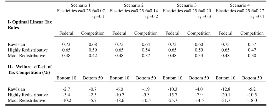
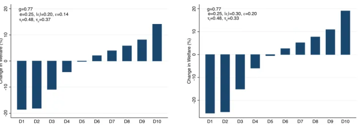
2.4.2 Results
The baseline results of the numerical calibrations are presented in Table1and Figure1using the French earnings distribution. I use as the baseline scenario a constant labour supply elasticity of 0.25 and a migration elasticity that is constant across earnings types, meaning that all the "i
have the same absolute magnitude. This implies that at all income levels, individuals have the same migration response to a change in their consumption caused by a change in taxes, except that tax changes have an opposite effect on individuals’ consumption depending on which side of the break-even point they are. Using the theoretical formulas of the optimal linear tax rates, I compute the optimal linear tax rates in the federal and the competing unions for different redis-tributive tastes and various values for the migration elasticity. Given these optimal tax rate, I use the first order condition of the individual problem together with the exogeneous skills distribution to compute their optimal amout of labour supply and pre-tax earnings under each tax systems and
scenarios. The transfers for each tax systems and scenarios are determined by the sum of these pre-tax earnings. I finally compute the welfare of individuals under each tax system using the utility specification presented in Equation (8). The welfare effect of tax competition is given by the change in welfare from going from a federal union to a competition union. These changes are summarized for the bottom ten and fifty percent in Table1. I show the full distribution of welfare gains and losses created by tax competition across all earnings deciles in Figure1. In TableB.III, I relax the assumption of constant elasticities and investigate the special case where tax-driven migration is only present at the top of the income distribution.
3 Non Linear Tax Schedule with Discrete Income Brackets
To take into how the tax progressivity of tax systems may be affected by the presence of tax competition, I develop a discrete version of the Mirrlees model, followingPiketty[1997] andSaez
[2002], in the presence of migration. The discrete non linear case has the advantage to be more tractable than the non linear model with continuous types, and to shed light on marginal tax rates at in the top and bottom brackets. Compared to the linear analysis developed before, it also allows to better take into account how the progressivity of the tax system can be affected by the magnitude and the distribution of migration elasticities.
3.1 Baseline Framework
Agents are indexed by k and are endowed with continuously distributed skills wk, but there is a
finite numbers of tax brackets, or occupations, i = 0,...,I. Each tax bracket provides a wage yifor
i= 0,..,I , with y0 = 0. Earnings yi are increasing with i, and I start by assuming that there is
a perfect substitution of labour types in the production function, implying that pre-tax wages are fixed. The government cannot directly observe individuals’ skills and has to condition taxation on the observable income levels. The tax function is non-linear, and depends on the level of earnings, such that individuals in bracket-i have an overall tax liability T (yi) = Ti.
Similarly than before, individuals have a utility function uk(c
i, k(i)) that is a function of their
tax-bracket choice k(i) and the after-tax income level in their bracket ci. Given their abilities,
maximize their utility. There is a population hiof agents in each bracket i 2 I + 1, and Âihi= N
is the total population in the country. As in the linear model, agents respond to distortions created by taxation through labour supply changes, that are captured by their choices of income brackets. Labour supply decisions of individuals are thus loaded in the function hi(c0, c1...., cI). I assume
that the tastes for work embodied in the individual utilities are smoothly distributed so that the aggregate functions hi are differentiable. As before, I consider as an important simplification the
case with no income effects. In this case, increasing all after-tax consumption levels by a constant amount does not affect the distribution of individuals across brackets.
In this model, T (yi) embeds all taxes and transfers received by each individual. Compared
to the simplistic linear case studied before, the more complex non-linear tax schedule allows to explore at a finer level variations in the profile of transfers depending on the level of revenues. The non-linear tax system is characterized by two key concepts. First, the universal demogrant T(0) = T0 that is distributed to everyone. Second, the marginal tax rate T0(yi) that captures the
taxation on transitions from one bracket to another. The marginal tax rates, also called the phasing-out rates, allow to take into account the distributive effects of income taxation in the presence of behavioural responses to taxation. It also allows to capture at which rate the lumpsum grant is taxed away, and how the tax liability increases with earnings. A negative value for Ti(yi) means
that individuals receive a net transfer from the government, and has to be distinguished from a negative value for the taxation rate on occupations transitions defined by (Ti Ti 1)/(ci ci 1).
There is an i for which Ti= 0, and as in the linear case I call this income level the break-even point.
An important feature of the optimal tax problem is that it does not produce an explicit formula for the optimal transfer -T(0). The guaranteed income is determined in general equilibrium, and results from the optimal tax and transfer schedule Ti, and the empirical densities hidetermined by the tax
schedule. The amount of taxes and transfers in each bracket Ti are set by the government in order
to maximize a total welfare function. The government budget constraint is a function of the tax schedule and the endogeneously determined density of individuals in each income bracket:
R=
I
Â
i=0hiTi (9)
be considered regarding the optimal tax problem. I start by studying a revenue-maximizing gov-ernment. Then I consider a government that maximizes the total welfare in the economy, using the concept of generalized social welfare weights, where gicaptures the weight given to additional
consumption for individuals in the tax bracket i, as in the linear analysis.
I extend the model to the case where individuals can react to taxation with migration. Similarly than in the linear model, in the presence of tax competition, taxation affects individuals’ choices at the intensive margin regarding their choice of income bracket, and at the extensive margin through their migration choices. Conditional of being in the bracket i, individuals choose to migrate from A to country B if their utility is higher in country B. The migration condition considered in the linear case is unchanged, except that the tax system is now non-linear, and Ti directly loads the
total tax liability of type-i individual:
uAi = yi TiA vi(yi, li) + ✓iA m (10)
ui(cAi , yi, ✓Ai , m) ui(cBi , yi, ✓Bi , m) (11)
As before, the migration condition establishes that location choices are driven by differences in tax liabilities between the two countries, and the density of individuals in one country is therefore a function of its tax liability in this country. As in the linear framework, in the presence of tax competition the number of individuals in the national bracket i becomes a function of the tax and transfer schedule in this country hi(ci). Migration decisions are thus driven by average tax
liabilities, by contrast to occupation decisions that are driven by taxation on transitions from one bracket to another. The migration responses to taxation can be summarized in terms of elasticity concepts. By contrast to the linear case, individuals’ consumption does not depend on a net-of-tax average rate, but of the amount of taxes paid and transfers received Ti. Therefore, I define the
migration elasticity as the change in the density of type-i individuals locating in country A when their disposable income in country A is increased by one percent:
⇠i=@hi
@ci ⇥
ci
hi (12)
for individuals with income levels below the break-even point. As I define the migration elasticity with respect to consumption in the linear case, it is positive at all income levels.
3.2 Intensive Model
In this section, I present the canonical intensive model first developed byPiketty[1997] andSaez
[2002] where individuals respond to taxation through labour supply choices only. In this model, a change in consumption level in any bracket i relative to another bracket i 1 induces individuals to switch from bracket i to bracket i 1. For simplicity, I assume that agents can only choose between adjacent occupations, and therefore, hiis only a function of ci, ci+1and ci 1. I define the
elasticity of the number of individuals in bracket i with respect to the differences in consumption ci ci 1
⌘i=@(c @hi i ci 1) ⇥
(ci ci 1)
hi (13)
As outlined byPiketty[1997], ⌘icaptures the transition of individuals to bracket i 1 to bracket
i when the difference in consumption between the two brackets is increased. The parameter ⌘i
captures the participation of each individual in bracket i, and can be easily linked to the earnings elasticity ei. Following Saez [2002], I use the relationship ⌘iyi = ei(yi 1 yi). Hence, with
intensive responses at the labour supply margin, a change in the tax liability in the bracket i will affect the transition rate between the bracket i and the adjacent occupations. The maximization of the government tax revenue leads to the first order condition:
hi= Ti 1@(c@hi 1 i ci 1) Ti+1@(c@hi+1 i+1 ci)+ Ti @hi @(ci ci 1) Ti@(c @hi i+1 ci)
The optimal tax liability of the revenue-maximizing government is given by: Ti Ti 1
ci ci 1 =
hi+ hi+1+ ... + hI
hi⌘i (14)
The proof is formally derived in the Appendix A.4.1. Using ⌧i the implicit marginal tax rate
on bracket i such that ⌧i= (Ti Ti 1)/(Yi Yi 1), where 1 ⌧i= ci ci 1/Yi Yi 1, and ai=
where individuals can only respond to taxation through labour supply choices. This corresponds to the case of a federal government composed by symetric countries. When countries set the same tax and transfer schedule and are symetric such that before-tax salaries are equal, there is no differences in consumption between home and abroad that is affected by taxation. Therefore, migration decisions are independent from Ti, and do not affect the optimal tax formula.
Proposition 3. Optimal Marginal Tax Rate of the Revenue-Maximizing Federal Government: ⌧if = hi+ hi+1+ ... + hI
hi+ hi+1+ ... + hI+ hiaiei (15)
Proof. The proof is formally derived in the Appendix.
As outlined by Saez [2002], in the absence of extensive margin responses to taxation, the optimal tax liabilities are always increasing with i, and negative marginal tax rates are therefore never optimal.5 As a result, the marginal tax rate in the first bracket is very high, and is maximal in
the Rawlsian case with high redistributive taste. In complement to the formal maximization of the government problem given in the Appendix, it is possible to provide a simple and intuitive proof of Equation15by studying a small deviation in the tax schedule. Consider a small change dT for all brackets i,i + 1,...,I. This change in taxation changes ci ci 1, leaving all other differences
in consumption levels unchanged. This change in tax liabilities induces a mechanical increase in collected revenue equal to (hi+ hi+1+ ... + hI)dT . The change in taxation also induces a
behavioral response through the change in transition from bracket i to i 1. Using the definition of the participation elasticity, the mass of taxpayers in bracket i changes by dhi= hi⌘idT /(ci
ci 1), inducing a loss in tax revenue of dhi(Ti Ti 1). Summing the behavioural and mechanical
effects to zero, we retrieve the formula for the optimal tax formula in the pure intensive model.
3.3 Extensive Model
I now turn to the extension of the canonical model, allowing migration responses to taxation. To emphasize how the tax driven mobility affects the non linear tax schedule, I start by considering 5The fact that negative marginal tax rates are never optimal would plausibly hold even considering participation margin at the bottom of the income distribution in that model. This is because the government is Ralwsian, which implies that the underlying welfare weights are very high for unemployed, and lower for poor workers.
the pure extensive model, where individuals can only respond to taxation through migration. This means that given their location decision, individuals’ earnings are fixed. The only effect of Tion hi
is therefore through migration responses to taxation summarized by Equation (10). The revenue-maximizing government chooses the optimal Ti taking into account the endogeneous changes in
hi due to migration responses to taxation, and the optimal tax and transfer schedule for type-i
individuals satisfies:
Ti
yi Ti =
1
⇠i (16)
The proof of Equation Equation (16) is derived in the Appendix. I give a simple intuition of the formula studying a small deviation in the tax schedule when individuals respond to taxa-tion through migrataxa-tion only. In the pure extensive model, the change in tax liability Ti has an
effect on migration decisions of individuals in bracket i, but does not affect transition to adjacent brackets. The change in Ti produces a mechanical increase in collected tax revenue hidTi. The
reform also creates a behavioral effect through migration, with a change in taxpayers mass of dhi= hidTi/ci⇠i. Each individual emigrating from the country induces a loss of its overall tax
liability Ti, and the overall behavioral effect is therefore hidTi/ci⇠iTi. Summing behavioural
and mechanical effects to zero gives the formula for the optimal tax and transfer schedule for each income bracket i. The marginal tax rate from bracket i to bracket i 1 is therefore given by
Ti Ti 1 ci ci 1 = 1 ci ci 1( yi 1 + ⇠i yi 1 1 + ⇠i 1)
3.4 Optimal Linear Tax Rate in Tax Competition
I finally put together the pure intensive and extensive model to consider the case where individuals respond to taxation through migration and labour supply behavioural reponses. With a sligh abuse of notation, I rewrite the population function of taxpayers in the country as hi(ci ci 1, ci+1
ci, ci). The first two terms capture the effect of taxation on transition to adjacent tax brackets,
while the last term captures the effect of taxation on utility differentials between home and abroad through consumption at home ci. The derivation of the government tax revenue with respect to Ti
hi= (Ti Ti 1)@(c @hi i ci 1)+ (Ti+1 Ti) @hi @(ci+1 ci)+ Ti @hi @ci
Making use of the set of first order condition and the fact that @(c @hi
i ci 1)=
@hi 1
@(ci ci 1), I
ob-tain an expression for the optimal non linear tax rate chosen by a revenue-maximizing government in the competition union.
Proposition 4. Optimal Revenue-Maximizing Marginal Tax Rate in Tax Competition: ⌧ic= hi(1 bi⇠i) + hi+1(1 bi+1⇠i+1) + ... + hI(1 bI⇠I)
hi(1 bi⇠i) + hi+1(1 bi+1⇠i+1) + ... + hI(1 bI⇠I) + hiaiei (17)
Proof. The optimal tax rate formulas are formally derived in the Appendix.
The formula for the optimal non linear tax rate in tax competition can also be retrieved by using a small deviation in the tax schedule. I consider a small deviation dT for all tax bracket i, i+ 1,..I. As in the pure intensive model, this change in taxation modifies ci ci 1, leaving
all other differences in consumption levels unchanged. The change in tax liabilities induces a mechanical increase in collected revenue equal to (hi+hi+1+...+hI)dT . The change in taxation
also induces a behavioral response through the change in transition from bracket i to i 1. Using the definition of the participation elasticity, the mass of taxpayers in bracket i changes by dhi=
hi⌘idT /(ci ci 1), inducing a loss in tax revenue of dhi(Ti Ti 1). In the presence of tax
competition, there is an additional effect on tax revenue due to migration responses to taxation. As migration decisions are driven by overall tax liabilities, the change dT creates a migration response in all brackets affected by the change. Using the definition of the migration elasticity, the change in the number of taxpayers due to the tax reform can be written dT (hi
ci ⇠i+ hi+1 ci+1⇠i+1...+ hI cI ⇠I).
Any individual migrating from the country imposes a loss in tax revenue equal to its overall tax liability, such that the effect of tax-driven migration on tax revenue is equal to dT (hi
ci
Ti⇠i+
hi+1
ci+1Ti+1⇠i+1...+
hI
cITI⇠I). Note that by contrast to the linear case, the revenue and transfer
channels are simultaneously captured by the overall tax liability Ti, that can either be positive or
negative. Summing the behavioural and mechanical effects to zero yields the optimal tax formula. Letting one of the two elasticities eiand ⇠itend to zero in Equation (17), we retrieve the optimal
fundamental parameters that relate to the two distortions implied by the intensive and extensive behavioural responses to taxation. The labour supply responses is weighted by the discrete equiv-alent of the usual Pareto parameter ai = Yi/(Yi Yi 1) that captures the relative gain from the
income bracket transition taxed at the marginal rate ⌧i, while the migration response is weighted
by the parameter bi= Ti/(yi Ti), emphasizing how location choices are driven by average tax
rates. The migration wedge bi is negative for individuals with income level below the break-even
point, leading the overall migration response bi⇠i of bottom earners to be negatively weighted in
the optimal tax formula, making the link between the optimal tax formula derived in the linear framework.
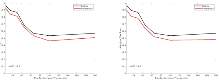
The optimal marginal rates in the discrete linear case are, as it is well known, U-curved, with high and decreasing marginal rates at the bottom of the distribution, and increasing marginal rate at the top of the distribution. Of particular interests are the optimal top and bottom marginal tax rates. The optimal formulas in Equation (17) relate to the extreme case of a revenue-maximizing government, where the social planner exclusively values redistribution towards zero earners. As emphasized byPiketty and Saez[2013], this specific case of social preferences is likely to generate high values for the optimal bottom marginal tax rate ⌧1. This is because increasing the transfers
by increasing the phase-out rate produces a moderate behavioral cost, as individuals who decide to leave the labor force would have had low earnings should they work. As a result, in the presence of extensive and intensive responses to taxation, the optimal phase-out rate chosen by the Ralwsian government is positive, and very high.
As emphasized by Proposition4, tax competition modifies the optimal tax and transfers sched-ule compared to the federal system summarized by Proposition3, to an amount that is proportional to the migration tax wedges bi that are negative for low income levels, and the mobility
elastic-ities ⇠i. In the non-linear case, the effect of migration on the universal demogrant through the
amount of taxes paid and the amount of transfer received is directly loaded in the term Ti that
captures the net amount of taxes and transfers received or paid by the individual in bracket i. To simply illustrate this fact, and link the migration wedge bito the trade-off between the income and
population weighted mobility parameter faced by the government in the linear case, I present the derivation of the optimal non-linear tax rate in the presence of migration by making the distinction between the amount of taxes paid ˜Ti and the amount of transfer received by everyone T0. The
resulting optimal linear tax rate is the same than the one presented in Proposition 3 with alter-native notations. In this case, the government seeks to maximize 1
ÂihiÂihi
˜
Ti, where the total
number of taxpayers N =Âihiis endogeneously affected by the tax schedule through migration
responses to taxation. With N =Âihiand R =ÂihiT˜i, the first order condition of the government
with respect to the amount of taxes ˜Ti can be rewritten as 1
N2( @R @ ˜Ti ⇥ N @N @ ˜Ti⇥ R) = 0 which is equivalent to @R @ ˜Ti =@N @ ˜Ti⇥ R
N. Intuitively, the government first order condition with respect to ˜
Ti indicates that at the optimum, the change in tax revenue due to a distortion in type-i
individ-uals tax liability has to be offset by the change in transfer caused by the change in the number of type-i taxpayers implied by the tax reform, such that the net effect of the reform is equal to zero in the optimum. As before, I consider a small change d ˜T on tax brackets i,i + 1...,I. The change d ˜T causes a change in the density of taxpayers in all brackets affected by the tax reform that is equal to d ˜T( hi⇠i
ci
hi+1⇠i+1
ci+1 ... hI
⇠I
cI). Each migration response to taxation induces
a fiscal lost equal to individual’s overall tax liability. When the absolute number of taxpayers is changed by the small tax deviation, there is an additional effect of migration on the government tax revenue, through the change in the number of transfers’ benificiaries, and each individual em-igration yields a fiscal gain equal to the universal demogrant T0= T (0). It follows that the net
effect of migration responses to taxation of d ˜T is equal to d ˜T(hi⇠i
ci( ˜Ti T0) + hi+1
⇠i+1
ci+1( ˜Ti+1
T0) + ... + hI⇠I
cI( ˜
TI T0)). The overal effect of d ˜T on the universal demogrant is therefore
d ˜T(hi+ hi+1+ ... + hI Ti Ti 1 ci ci 1hi⌘i ⇠i ˜ Ti T0 ci hi ⇠i+1 ˜ Ti+1 T0 ci+1 hi+1 ... ⇠I ˜ TI T0 cI hI).
The mobility response of individuals in each bracket-i is weighted by bi= ( ˜Ti T0)/ci= Ti/ci,
meaning that the trade off between the revenue and the transfer channel of tax driven migration responses emphasized in the linear case is captured by the migration wedge bi in the non linear
case.
3.5 Welfare Weights
I finally turn to the derivation of the optimal non linear tax tax and transfers schedule relying on the more general concept of generealized social marginal welfare weights. These formulas will be used in the numerical simulations, as they allow to capture the effects of government’s tastes for
redistribution on the optimal tax rates, and ultimately on the welfare effects of tax competition. As I will show later, the formulas of the optimal non linear tax rate with discrete earnings and welfare weights allow to emphasize simply the effects of tax-driven mobility on redistribution. I use the concept of generalized marginal social welfare weights, to be fully consistent with the approach presented for the linear framework. As before, the government attributes a weight gito
type-i individuals’ consumption, and the optimal tax schedule is such that any small tax deviation is welfare neutral.
Proposition 5. Optimal Non-Linear Marginal Tax Rates in Federal Union: ⌧if = hi(1 ¯gi) + hi+1(1 ¯gi+1) + ... + hI(1 ¯gI)
hi(1 ¯gi) + hi+1(1 ¯gi+1) + ... + hI(1 ¯gI) + hiaiei (18)
Proof. With ¯gi= gi/(ÂIm=0hmgm⇥ N). The proof is derived below.
Proposition 6. Optimal Non-Linear Marginal Tax Rates in Tax Competition:
⌧ic= hi(1 bi⇠i ¯gi) + hi+1(1 bi+1⇠i+1 ¯gi+1) + ... + hI(1 bI⇠I ¯gI)
hi(1 bi⇠i ¯gi) + hi+1(1 bi+1⇠i+1 ¯gi+1) + ... + hI(1 bI⇠I ¯gI) + hiaiei (19)
Proof. With ¯gi= gi/(ÂIm=0hmgm⇥ N). The proof is derived below.
As in the linear case, I derive the optimal non linear tax rate using the small perturbation method with generalized social marginal weights, where the optimal tax schedule is such that no welfare gain can be acchieved through a small reform.6 Consider again a small tax devi-ation dT on tax brackets i,i + 1...,I. The devidevi-ation causes a mechanical increase in tax rev-enue dT (hi+ hi+1+ ... + hI). In addition to the mechanical change in revenue collected due
to the tax reform, the small tax deviation creates behavioural responses to taxation. In the federal union, there is no migration responses to taxation, and the only behavioural response to taxation is through labour supply responses to the tax reform. The tax reform dT modifies transition to bracket i 1 to bracket i, and the density of taxpayers in the bracket i is changed by the amount dhi = hi⌘idT /(ci ci 1) at a net fiscal cost (Ti Ti 1). The total effect of the reform on
6SeeSaez and Stantcheva[2016] for a discussion on the local derivation of the optimuum with generalized social marginal weights.