HAL Id: cea-02519732
https://hal-cea.archives-ouvertes.fr/cea-02519732
Submitted on 26 Mar 2020
HAL is a multi-disciplinary open access
archive for the deposit and dissemination of
sci-entific research documents, whether they are
pub-lished or not. The documents may come from
teaching and research institutions in France or
abroad, or from public or private research centers.
L’archive ouverte pluridisciplinaire HAL, est
destinée au dépôt et à la diffusion de documents
scientifiques de niveau recherche, publiés ou non,
émanant des établissements d’enseignement et de
recherche français ou étrangers, des laboratoires
publics ou privés.
System Level Analysis for ITS-G5 and LTE-V2X
Performance Comparison
Pierre Roux, Stefania Sesia, Valérian Mannoni, Eric Perraud
To cite this version:
Pierre Roux, Stefania Sesia, Valérian Mannoni, Eric Perraud. System Level Analysis for ITS-G5 and
LTE-V2X Performance Comparison. IEEE MASS 2019 - The 16th IEEE International Conference on
Mobile Ad-Hoc and Smart Systems, Nov 2019, Monterey, United States. �cea-02519732�
System Level Analysis for ITS-G5 and LTE-V2X
Performance Comparison
Pierre Roux
Communicating Systems Lab CEA, LIST
Gif-sur Yvette, France [email protected]
Stefania Sesia
Strategy Office Renault Software Labs Sophia Antipolis, France [email protected]
Valerian Mannoni
Smart Objects Communication Lab CEA, LETI
Grenoble, France [email protected]
Eric Perraud
Strategy Office Renault Software Labs
Toulouse, France [email protected]
Abstract—Vehicular communications, known under the name of V2X (Vehicle to Everything) are expected to grow fast in the next years, bringing for example safer driving conditions, optimized traffic management, energy reduction, etc.. Currently two short range-based technologies (ITS-G5, standardized in Europe by ETSI and derived from WiFi communications IEEE standards and LTE based Vehicle to Everything or LTE-V2X developed by 3GPP and derived from LTE) consider the use of 5.9 GHz ITS band for their deployment. While different countries are more or less advanced in terms of regulation definition for Intelligent Transport System (ITS), it seems clear that the same solution will not be necessarily worldwide deployed. This study compares performances of both technologies by means of system level simulation, in particular considering the European ITS-G5 protocol stack specification. In order to analyze system level performance, physical layer simulation is used to provide Packet Delivery Rate (PDR) versus Signal to Noise plus Interference Ratio (SINR). Then PDR curves are exploited to feed system level simulation aimed at providing statistics about Cooperative Awareness Message (CAM) transmission reliability, in typical urban scenario. The paper provides a brief description of the systems together with the definition of the assumptions and the key results related to the physical layer analysis; it follows with the description of the NS-3 simulator models used for system level simulation (with particular emphasis on PC5 Mode 4) and the discussion about the results which provide insight about the expected and the simulated behavior of both technologies, in particular comparative statistics with regards to CAM success ratio versus maximum communication distance are provided in order to compare the performance.
Index Terms—vehicle communications mobility performances
I. INTRODUCTION
Vehicular communications have been identified as a key enabler for improving vehicular safety, traffic and energy efficiency as well as the quality of the user experience, for automated and autonomous vehicles.
Different type of communication links are introduced in the standard such as Vehicle (V2V), Vehicle-to-Infrastructure (V2I) which is based on the use of short range technology and Vehicle-to-Network (V2N) communications which is based on long range technology such as LTE. Those type of links are generally referred to as Vehicle-to-Everything (V2X).
Short range communication is based in Europe on the ‘Intel-ligent Transportation System (ITS)-G5’ protocol developed by the European Telecommunications Standards Institute (ETSI).
Moreover, the access layer which has been included in the European “Delegated Act’ is based on IEEE 802.11p for vehicular networks.
In addition, the fast development of LTE cellular systems has evolved towards vehicular communications applications. 3GPP Release 14, extends therefore the Proximity Services (ProSe) functionality by adding two new modes, Modes 3 and 4, for LTE based vehicle-to-everything (here called LTE-V2X) connectivity [1]. Modes 3 and 4 of LTE-V2X have been designed to satisfy specific requirements in terms of latency and to accommodate high levels of density of vehicles com-bined with high Doppler spreads. Mode 3 uses the centralized base station (eNB) scheduler for efficient resource scheduling, while Mode 4 is purely based on side link autonomous and distributed resource selection algorithm, hence requiring no support or control from a cellular eNB. In this paper, we will consider only PC5 mode 4, because mode 3 is not foreseen to be deployed on the short term.
While IEEE 802.11p is a rather mature technology, whose capability has been tested in a large number of test beds since many years, LTE-V2X is more recent with first trials performed during 2018 only based on prototype solutions while commercially available modules have been only very recently released, hence only few comparisons exist which gives insight about the benefits and limitations of the different systems.
In addition, it is not easy to test in realistic scenarios the behaviour of the systems for growing density of users. Hence, it is important to analyse system performance comparison between the two technologies under various simulated con-ditions.
In [2] Annex A, use cases are proposed for evaluating vehicle communication systems with well defined performance evaluation scenarios. In [1], this annex is used as a starting point in order to evaluate the performances of LTE-C2X at system level.
The objective of this paper is to propose a fair comparison of both standards by evaluating both the lower layers and protocol stack performance. System level simulations are based on [2] annex A again, however this common ground is used for evaluating both technology candidates (ITS-G5 and LTE-V2X) under identical use case and methodology for performance
evaluation.
In the following, Section II briefly introduces the physical layer parameters and the simulation comparison. Extended analysis can be found in [3].
Section III introduces system level simulation set up based on urban topology, and Cooperative Awareness Applications (based on CAM messages); it describes the system level simulation principles with a specific focus for each technology in Section III-D for LTE-V2X and Section III-E for 802.11p and it provides the system level performance evaluation. Section IV discusses the comparison between both the tech-nologies. Finally Section V draws the conclusions.
II. V2X PHYSICAL LAYER PERFORMANCE ASSESSMENT
In this section, we first present the physical layer of the V2X communication systems and the simulation results for the physical layer considering a point-to-point link are then illustrated. These results at the physical layer level will then be integrated into the network simulator in the form of Look-Up Tables (LUT).
A. V2X Physical layer
The IEEE 802.11p physical layer is an evolution of IEEE 802.11a. It uses Orthogonal Frequency Division Multiplexing (OFDM) combined with a convolutional code [4]. To provide performance under rapidly varying channels, the time domain parameters have been doubled, while the frequency domain parameters have been halved. The typical parameters are given in Table I. A description of the IEEE 802.11p physical layer can be found in [4].
The C-V2X physical layer defined in [5] is based on Single Carrier Frequency Division Multiplexing Access (SC-FDMA) and supports 10 or 20 MHz channels. Each channel is divided into sub-frames, Resource Blocks (RBs), and sub-channels.
The same numerology as in LTE is considered with a 1 ms long subframe and a RB corresponding to 180 kHz (i.e. 12 sub-carriers each of 15 kHz spacing) and 0.5 ms in time. C-V2X defines sub-channels as a group of contiguous RB pairs in the same sub-frame. Sub-channels are used to transmit data and control information. The data is transmitted in Trans-port Blocks (TBs) over Physical Sidelink Shared Channels (PSSCH), and the control information (MCS, RBs, ressource reservation interval) in Sidelink Control Information (SCI) messages over Physical Sidelink Control Channels (PSCCH) [6] and sent within the same sub-frame. A node that wants to transmit a TB must also transmit its associated SCI. As for LTE, the control information SCI is critical as it allows to receive and decode the transmitted TB.
TBs can be transmitted using QPSK or 16-QAM modu-lations with a set of coding rates which are defined by the Modulation and Coding Scheme (MCS) in [6], whereas the SCIs are always transmitted using QPSK with MCS=1. Unlike IEEE 802.11p, C-V2X is based on turbo coding, except for SCI which is convolutionnaly encoded.
The considered parameters are given in Table I. Compared to IEEE 802.11, C-V2X provides more flexibility in terms
TABLE I
IEEE 802.11P VERSUSC-V2X, PHYLAYER MAIN TYPICAL PARAMETERS
IEEE 802.11p C-V2X Sampling Frequency, Fe(Fe) 10MHz 15.36MHz
Tone Spacing, ∆f 156.25kHz 15kHz FFT Size, NF F T 64 1024
Symbol Duration, Ts 8µs 66.67 µs
Number of data subcarriers, Nu 48 12×RB
Cyclic Prefix Size, Ncp 16 (1.6µs) 72 (4.7µs)
Modulation QPSK QPSK / 16QAM Forward Error Correction CC TC
Coding Rate, Rc ½ from MCS
Transmit power 23dBm 23dBm
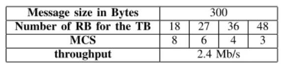
of configuration: occupied bandwidth, modulation and coding scheme can be selected at physical layer as well as a set of parameters at MAC layer. This allows to adapt transmission according to the surrounding conditions e.g. adapting the transmission to available resources, or to the congestion level. In our simulations, we considered a subset of the possible configurations that are given in Table II for a message of 300 Bytes which stems from a set of possible configurations according to 3GPP numerology, within the ranges standardized in [6], satisfying the congestion control constraints as defined in [7] and taking into account the typical packet size of a CAM message.
B. Physical layer results
The results in this section are provided in terms of Packet Error Rate (PER) versus SNR or range for both IEEE 802.11p and C-V2X. Throughout the paper, we consider the Extended Vehicular Model EVA channel model as defined in [8]. Several configurations are considered for C-V2X. It should be noted that in this paper we consider perfect channel estimation for both technologies.
TABLE II
C-V2XPHYSICAL LAYER CONFIGURATIONS WITH RESULTING THROUGHPUT(SIGNALING INCLUDED)
Message size in Bytes 300 Number of RB for the TB 18 27 36 48
MCS 8 6 4 3
throughput 2.4 Mb/s
Fig. 1 gives the link performance for C-V2X and ITS-G5 for the considered message size of 300 Bytes and assuming a speed of 120 km/h. As expected, the C-V2X results show that the parameterization that uses the largest number of RBs (larger bandwidth) outperforms other configurations thanks to the possibility to exploit frequency diversity and to use a lower coding rate (lower MCS) compared to narrowband allocations. The performance when 1 retransmission is used is also illustrated for C-V2X. We can then observe a gain between 5 and 8 dB in terms of SNR thanks to the additional coding gain.
This gain comes from the combination of redundancy (coding gain) and better time diversity of the propagation channel.
Fig. 1 shows that the SNR for a P ER = 10−2 varies from 3.4 to 12.4 dB when single transmission is considered and between −1.7 and 4.3 dB when a blind retransmission is used. For a given signal bandwidth of 10 MHz (48 RB and MCS=3 for C-V2X) and only one transmission, C-V2X outperforms ITS-G5 with a gap of 7.2 dB for a P ER = 10−2. That is mainly explained by the difference in data rate (4.7Mb/s for ITS-G5 and 2.4Mb for C-V2X) and also by the difference in terms of coding rate. It should also be noted that the C-V2X uses a Turbo-code which has per definition better performance than the convolutional code used by ITS-G5.
Fig. 1. ITS-G5 and C-V2X PER as a function of the SNR in EVA channel for a message of 300 Bytes at 120 km/h
A performance synthesis using more physical layer config-urations in particular for C-V2X is given in [3].
III. SYSTEM LEVEL SIMULATION
A. The urban use case
Our target is to evaluate the performance of a given technol-ogy by providing statistics about successful communications of Context Awareness Messages (CAM) from sender vehicles to receiver vehicles. However the provided statistics should only include communications for which the distance between sender and receiver is lower than a reference distance which is used as the x-coordinate. This criterion is proposed in the annex A of TR 36.885 ( [2]). We also adopt here the urban scenario that is proposed in [2] for evaluating performances of a given vehicle communication technology. Other scenario are introduced in [2] as well but this one is the most challenging because of the density of vehicles on one side and also because of the presence of buildings that introduce a large amount of non line of sight radio communications.
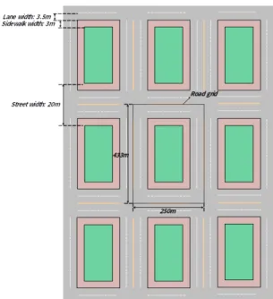
Figure 2 shows the road configuration for the urban sce-nario. We have an urban area of size 750x1399 meters with 9 buildings, and roads between buildings, with 2 lanes in each direction for each road. Vehicles are moving in this area at equal constant speed. At road intersection, vehicles may go either straight (with probability 0.5) or left (with probability 0.25) or right (with probability 0.25 again).
We use wrap around in order to avoid border effects. This area is considered as one tile that is repeating itself inside
Fig. 2. Road and building configuration for urban case (extracted from [?])
an infinite 2D grid. Vehicles leaving the area on the left (respectively right, top, bottom) are re-entering the area on the right (respectively left, bottom, top).
Wrap around also applies on how geographic distances are calculated, e.g. a vehicle located on the extreme left of the area is very close to another vehicle on the same horizontal lane that is located at the extreme right of the area.
If the direct line between 2 vehicles is crossing any building, then we have Non Line of Sight conditions (NLOS). On the contrary if no building is crossing the line, then we have Line of Sight conditions (LOS).
A path loss model is also suggested in [2]. The ”Winner B1” path loss model (as described in Table 4-4 of [9] is proposed, with different formulae for addressing either LOS or NLOS conditions. This Winner B1 path loss model is the one used in the current study.
Vehicles are initially located on random lanes and at random positions. Then vehicles are moving at constant speed and may change of lanes if they turn left or right. However the number of vehicles that are introduced in the area depends on the selected speed because the average distance between 2 neighbor vehicles on the same lane should be equal to the distance travelled during 2.5 seconds.
Two different vehicle speeds are suggested in [2] for running simulations: either 60 km/h in case of smooth urban traffic or 15 km/h in case of slightly congested urban traffic. Given the above constraint about average distance between neighbor vehicles, we have either 1476 vehicles in the area if the speed is 60 km/h, or 5902 vehicles of the speed is 15 km/h. B. Simulating CAM transmissions
A Context Awareness Message (CAM) rate of one message per second is assumed when the vehicle speed is 15 km/h. When the speed is 60 km/h we have a vehicle density divided
by 4 and a vehicle speed multiplied by 4, as shown in Table III.
TABLE III
MAIN SIMULATION PARAMETERS
If speed=15 km/h If speed=60 km/h Number of vehicles 5902 1476
CAM size 300 bytes 300 bytes CAM period 1 s 250 ms
A constant CAM size of 300 bytes is assumed in the current study. It is the average CAM size based on logs which have been captured on real live tests. Though longer messages could be considered in specific circumstances this simple assumption aims at simplification.
Both LTE-V2X and ITS-G5 can be used with Decentralized Congestion Control (DCC) algorithms. When they are used, all vehicles are responsible for sensing their communication channel and adapt their message transmission frequency in order to maintain the channel busy ratio at reasonable levels. However the current study doesn’t introduce any DCC. CAM transmission period is maintained at a value which depends on the vehicle speed as shown in Table III.
C. System level simulation principles
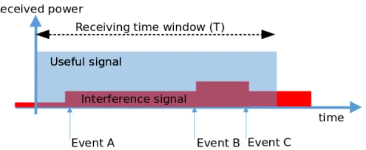
Whenever a sender vehicle has finished sending a message, all other vehicles make an attempt to receive this message. This message is called reference message here after. The period of time it took for sending this message is called T, as shown in Figure 3
Fig. 3. Calculating SINR in a receiving vehicle
The period T is typically short enough for neglecting the changes of position of the moving vehicle during T, so that the useful signal in blue in Figure 3 is represented as a constant. The same stands true for interfering vehicles. The level of interference of any interfering vehicle can be considered constant during T whenever this vehicle is sending.
However in the general case the activity of interfering vehicles is not synchronous with T. Events are occurring during T such as ”interfering vehicle starting transmission” or ”interfering vehicle stopping transmission. As an example in Figure 3 event A corresponds to some vehicle starting transmission, event B corresponds to some other vehicle starting transmission, and event C corresponds to some vehicle stopping transmission.
The successful reception of a message is based on the SINR value (Signal to Interference plus Noise Ratio) as computed for each receiver over the receiving window.
The useful received signal power is based on the transmitted power (which is a constant in the simulation, 23 dBm) and based on the path-loss calculation between sender and receiver, (which is depending on the distance between sender and receiver, and also on LOS or NLOS conditions).
The received interference power comes from other sending vehicles active at least partly during the transmission time of the reference sender (T). Interfering vehicles are transmitting at the same transmission power (23 dBm). The received interference power is calculated as the sum of contributions from all interfering vehicles, given the Winner-B1 path-loss between each interfering vehicle and the reference receiving vehicle.
In the optimistic version, a weight lower than 1 is applied on each interfering contribution, based on the ratio of time that is was active during the receiving window T. As an example, if an interfering vehicle was active during the last thirsd of T, a weight equal to 1/3 would be applied. On the contrary in the pessimistic version, all weights are equal to one, even though interference contributions were not always active during T.
The noise power is calculated with the well known formula FkTB (with F=noise factor, e.g. 9 dB, k is the Boltzman con-stant, T is the absolute temperature and B is the bandwidth).
A Packet Delivery Ratio (PDR) is derived from the com-puted SINR and from performances provided by physical layer simulations.
Finally the decision regarding reception success or failure is taken randomly (dice rolling) according to the computed PDR.
However we should notice that performances obtained from physical layer simulations may depend on vehicle speeds. Therefore at each time we consider a receiving vehicle that attempts to decode a V2X message, we should consider the relative speed between the sending and the receiving vehicles. In the urban scenario we have a limited number of cases for the relative speed:
• both vehicles move in the same direction, the relative speed between vehicles is zero.
• vehicles move in opposite directions, the relative speed is twice the vehicle speed.
• vehicles move in perpendicular direction, the relative speed is equal to the vehicle speed multiplied by√2 D. System level simulation applied to LTE-V2X simulation
V2X refers to vehicle to everything communications. How-ever we put the focus here on vehicle to vehicle communi-cations, through the 3GPP PC5 interface. When referring to 3GPP release 14 and later releases, this interface proposes four different communication modes. The present study only addresses PC5 mode 4, that allows direct vehicle to vehicle communications without any support from the cellular infras-tructure.
In the context of the PC5 interface, vehicle to vehicle com-munications assume a common synchronization source among vehicles. When referring to PC5, mode 4 this synchronization source is typically involving the vehicle’s Global Navigation Satellite System (GNSS). All communicating vehicles share a common understanding of time boundaries for Transmission Time Intervals (TTI) that last 1 millisecond each. Each TTI is an opportunity to transmit a Transport Block (TB) of data from one vehicle to another.
The principles exposed earlier for system level simulation can be simplified in such synchronous context. Both useful signals and interfering signals are synchronous. If 2 or several vehicles attempt to transmit a TB in the same TTI (and in the same resource), each vehicle will behave as an interference source for the other. There is no partial time interference for a receiver during any TTI.
Being based on Orthogonal Frequency Division Multiplex-ing (OFDM), PC5 mode 4 allows usMultiplex-ing different resources for communications, a resource being defined as a set of OFDM sub-carriers gathered in Resources Blocks (RB).
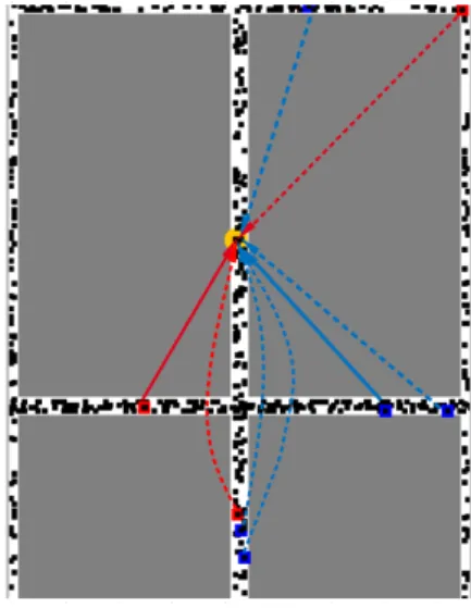
Computing a receiver SINR in this context should be done with reference to a given resource. This can be understood with reference to Fig. 4. It is assumed in the figure that we have defined 2 different resources. The first one is attached to the red color and the second one to the blue color. The figure shows a part of the simulation area with buildings shown in gray, and moving vehicles following lanes shown as black dots on the roads. The drawing refers to a particular TTI when a few vehicles are sending. Vehicles sending in the first (respectively second) resource are shown with a surrounding red square (respectively blue). Though all vehicles make an attempt to receive transport blocks in this TTI, the figure focus on one particular receiving vehicle which is shown in the middle of a yellow disk. This vehicle makes an attempt to decode a TB for each of the 2 possible resources. In the simulator, a different SINR value is computed for each resource.
A sending vehicle is carrying one Transport Block (TB) in one resource of a given TTI, together with its associated Sidelink Control Information (SCI). The SCI is typically using 2 out of the set of RBs that constitutes the resource, and contains information that the receiver needs for decoding the TB. In particular the Modulation and Coding Scheme (MCS) that the receiver needs for decoding the TB is included in the SCI (which is itself using MCS1).
Therefore a vehicle making an attempts to decode a TB is modelled according a multi-step process in the simulator:
1) Evaluate SINR for SCI decoding and TB decoding. We have different SINR values because the receiver bandwidth is different for both cases: SCI is using 2 RBs while the TB is using the other RBs in the resource. 2) Use SCI performance curves obtained from physical
layer simulation to derive a SCI decoding success prob-ability.
3) Draw randomly success or failure for SCI decoding, based on the above SCI error rate. If SCI decoding is failed, then the TB decoding is failed as well, otherwise
4) Use TB performance curves obtained from physical layer simulation to derive a TB decoding success prob-ability.
5) Draw randomly success of failure for TB decoding, based on the above TB error probability.
If performance curves obtained from physical layer simu-lation are depending on the relative speed between vehicles, then the appropriate curve should be selected in the process above, depending on the relative speed between vehicles.
Fig. 4. SINR calculation for PC4 mode 4
It is assumed that only one TB from a sending vehicle can be received in a receiving vehicle for each TTI and for each resource. Only the sending vehicle received with the maximum level in this TTI has a chance to be successfully decoded. This is just an assumption because some robust modulation schemes allows successful receiver decoding even with negative SINR values, however this assumption still makes sense in this context.
The sending vehicle received with maximum level is shown with a plain line in Figure 4.
PC5 mode 4 has introduced a scheduling mechanism for deciding when vehicles are allowed to transmit a TB at a given resource and TTI. This mechanism is known as the ”Sensing Based Semi-Persistent Scheduling (referred to later as SB-SPS). The principle consists in observing the channel in the receiver and deciding about short term periodic assignment for transmissions in such a way as to reduce potential collisions due to simultaneous transmissions of senders in the same TTI and resource (see [10] and [1] for exhaustive presentation).
Though many characteristics of the SB-SPS algorithm are fixed in the standard, a few of them can be configured. In this study, we have set the selection window (or maximum latency) to 100 milliseconds, and we have set the re-selection probability to 1 (which means that whenever the re-selection counter reaches zero, a new scheduling resource is selected). Two possible configurations for PC5 mode 4 are used in the present study, as shown in Table IV.
TABLE IV
PC5MODE4CONFIGURATIONS
Configuration 1 Configuration 2 Number of resources per TTI 1 2
Number of RBs per resource 50 20
MCS MCS3 MCS8
Size of CAM 300 bytes 300 bytes
Configuration 1 is using a robust Modulation and Coding Scheme (MCS3). However is provides only one resource per TTI. On the contrary, configuration 2 is using a less robust and less resource consuming MCS (MCS8) but it provides 2 resources per TTI.
Repeating SCI + TB over 2 TTIs (blind HARQ re trans-mission) is also an option for PC5 mode 4. This capability has been introduced in the simulator as well. However this mechanism and its simulation are not presented here, just because given the simulation parameters of table III, we have observed that repetitions are degrading rather than improving performances. Repetitions can only improve performances when we are far from congestion, which is not our case here. Note that DCC is supposed to make sure that repetition is not used whenever the Channel Busy Ratio (CBR) is high (e.g. when CBR is above 0,65 with a CAM size of 300 bytes). E. System level simulation applied to ITS-G5 simulation
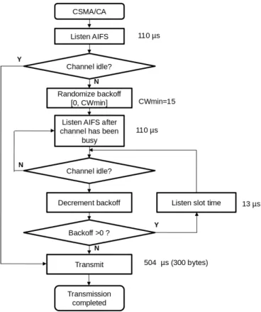
In the case of ITS-G5, CAM messages are sent by means of Carrier Sense Multiple Access with Collision Avoidance (CSMA/CA algorithm) in the broadcast mode. The state machine for CSMA/CA can be found e.g. in [12] at the Figure B.2. Figure 5 is reproducing this figure in the case of broadcast mode, together with detailed indications of the delay values used in our specific context.
Given this state machine for CAM message transmissions, the simulator for ITS G5 is not different from the one de-scribed earlier in the general case. No synchronous assumption can be done for ITS G5 (as opposed to what has been done for C-V2X) and the SINR computation should be done in the general case described in Figure 3 with the optimistic mode or the possibility to use either pessimistic or optimistic mode as described earlier.
F. Using ns-3 as system level simulator
ns-3 (https://www.nsnam.org) has been used as the system level simulator in this study. Being a discrete event network simulator, ns-3 is well fitted for simulating the non synchro-nized ITS G5 solution. It has been used as well for simulating PC5 mode 4, though a discrete event network simulator was not the only option in the context of this synchronized solution. A few ns-3 modules have been developed from scratch for the sake of our study:
• one ns-3 module for managing the Manhattan-like mobility involved in the urban scenario.
• one ns-3 module for facilitating the exploitation of PDR curves.
Fig. 5. State machine for ITS G5 CAM senders
• one ns-3 module for simulating PC5 mode 4 with a focus on the Sensing Based Semi Persistent Schedul-ing.
• and one ns-3 module for simulating the CSMA/CA broadcast algorithm of ITS G5.
Lookup tables have been used for determining LOS and NLOS conditions and for computing Winner B1 path losses. The use of lookup tables was motivated by the need to speed up simulation. Without such techniques, system level simulation involving a large number of vehicles are just too slow. Vehicle positions are first made discrete before any path loss computation, with a one meter granularity (so that the half maximum error is half a meter). Then pre-computed path loss matrices are used for retrieving path losses between two vehicles.
G. LTE-V2X performance evaluation
Figure 6 shows PC5 mode 4 Packet Delivery Ratio (PDR) performances in case we have MCS8, 2 resources per TTI, and a speed equal to 15 km/h. Two curves are shown: one with Sensing Based Semi Persistent Scheduling (SB-SPS) turned on and the other with SB-SPS turned off (in this sense that resource allocation is random instead of determined according SB-SPS algorithm).
Each curve provides the average PDR during simulation computed only on sender to receiver communications where the distance between sender and receiver is not exceeding to
the x-axis distance. This figure exhibits a significant perfor-mance improvement for the SB-SPS. If we consider a PDR equal to 0.9 as an example, activating SB-SPS pushes the x-axis distance from around 26 meters to around 34 meters.
Fig. 6. PC5 mode 4 PDR performances, 2 resources/TTI, speed=15 km/h
Figure 7 shows similar curves with the exception that only one resource per TTI is used. We still see significant im-provement because of SB-SPS, however the performances are slightly behind the former case with 2 resources per TTI. This might be considered weird because if remind configurations in IV we are now using a more robust MCS (MCS3 instead of MCS8). But the performances are dominated by the collisions phenomenon, and having 2 resources per TTI gives more resources to select from, and eventually less collisions.
Fig. 7. PC5 mode 4 PDR performances, 1 resource/TTI, speed=15 km/h
Now Figure 8 shows what happens with a speed equal to 60 km/h instead of 15 km/h. Though table III proposes to use a CAM period equal to 250 ms, we actually use a CAM period equal to 200 ms in this specific case because PC5 mode 4 is specified in such a way that only multiples of 100 milliseconds can be used for transmission opportunities.
We observe similar performances in Figure 8 as compared to Figure 6 so that the speed doesn’t make a lot of difference.
This makes sense because if we refer to III, when changing speed from 15 km/h to 60 km/h we also divide the number of vehicles by 4 in the same time that we multiply the CAM rate by 4 (or 5 in this specific case). At the end the data traffic due to CAM messages is not significantly different.
Fig. 8. PC5 mode 4 PDR performances, 2 resource/TTI, speed=60 km/h, CAM period=200 ms
H. ITS-G5 performance evaluation
We should first clarify if the choice between optimistic and pessimistic assumptions for SINR calculation is sensitive or not. Several simulations have been launched with respectively both options. In all cases it was shown that optimistic or pessimistic mode for SINR computation is never bringing any significant differences in terms of PDR performances. However we do not include such comparison results here for in order to keep the focus on the main outcomes.
Figure 9 shows PDR performances obtained for ITS G5 in both speed cases.
Fig. 9. ITS G5 PDR performances, speed=15 km/h and 60 km/h
We observe non significant differences between both speed cases. Again when going from 15 km/h to 60 km/h we divide the number of vehicles by 4, and we increase the CAM
message rate 4 times so that the CAM data traffic in the network is similar in both cases.
On Figure 9, we didn’t set any limit for the maximum tolerable latency. However with CSMA/CA we may have to wait for the channel to be silent (as shown in Figure 5. If the channel is close to congestion, this may involve non negligible waiting time.
Figure 10 provides latency-aware PDR performances. We have a set of curves in this figure, each curve being attached to a maximum tolerable latency. If a packet is received after this maximum latency is expired, then it is counted as a lost packet. The set of curves include maximum latency’s equal to 630 µs, 790 µs, 995 µs, 1255 µs, 1580 µs, 1990 µs, 2505 µs, 3155 µs, 3970 µs, and 5000 µs. The curve simply labelled ”PDR” is the one with infinite tolerance on the latency.
This set of curves shows that the curve with 5000 µs for maximum tolerable latency is difficult to distinguish from the curve with infinite tolerance. However we observe a non negligible sensitivity to maximum tolerance in the range below 5000 µs.
Fig. 10. ITS G5 PDR performances, speed=15 km/h various maximum tolerable latency’s
IV. COMPARISON BETWEENLTE-V2XANDITS-G5
SIMULATION
The PDR comparison for speed equal to 15 km/h is shown in Figure 11. If we consider a target PDR equal to 0.9, we observe that the x-axis range is pushed forward from 23 meters to around 35 meters when going from ITS G5 to PC5 mode 4.
The same general comparison for speed equal to 60 km/h is shown in Figure 12.
Though CAM period has been set to 250 ms in this figure (as required in Table III) it has been set to 200 ms for PC5 mode 4 because as already discussed. However even with a
Fig. 11. Compare all performances, speed=15 km/h
Fig. 12. Compare all performances, speed=60 km/h
slightly shorter CAM period, PC5 mode 4 is outperforming ITS G5.
V. CONCLUSION
The comparison of results between ITS G5 and PC5 mode 4 shows that PC5 mode 4 is out-performing ITS G5 in all cases. As an example, if we consider a target PDR equal to 0.9 and the urban scenario at speed 15 km/h the maximum distance is around 23 meters in case of ITS G5, and around 35 meters in case of PC5 mode 4. Furthermore if we consider latency maximum tolerance, the performance gap may only grow, because only ITS G5 may introduce latency when the traffic is high, while PC5 mode 4 is not introducing latency by design. However we may have to mitigate this conclusion if we remind that PC5 mode 4 supposes synchronization between vehicles, while ITS G5 does not require synchronization. Yet
the presence of GNSS in the vehicles is reducing the risk for lack of synchronization.
REFERENCES
[1] Rafael Molina-Masegosa and Javier Gozalvez, “System Level Evaluation of LTE-V2V Mode 4 Communications and its Distributed Scheduling” 2017 IEEE 85th Vehicular Technology Conference (VTC Spring) [2] 3GPP, “TR 36.885 Study on LTE-based V2X Services” v14.0.0, June
2016.
[3] V. Mannoni, V. Berg, S. Sesia and E. Perraud, “A Comparison of the V2X Communication Systems: ITS-G5 and C-V2X,” in 2019 IEEE 89th Vehicular Technology Conference, Kuala Lumpur, Malaysia, April 2019. [4] “IEEE Standard for Information technology-Telecommunications and information exchange between systems. Local and metropolitan area networks-Specific requirements. Part 11: Wireless LAN Medium Access Control (MAC) and Physical Layer (PHY) Specifications,” LAN/MAN Standards Committee of the IEEE Computer Society, Dec. 2016. [5] “3rd Generation Partnership Project; Technical Specification Group
Radio Access Network; Evolved Universal Terrestrial Radio Access (E-UTRA); Physical channels and modulation,” Release 15, 3GPP TS 36.211, v 15.2.0. June 2018.
[6] “3rd Generation Partnership Project; Technical Specification Group Radio Access Network; Evolved Universal Terrestrial Radio Access (E-UTRA); Physical layer procedures,” Release 15, 3GPP TS 36.213, v 15.2.0. June 2018.
[7] “Intelligent Transport Systems (ITS); Congestion Control Mechanisms for the C-V2X PC5 interface; Access layer part,” ETSI TS 103 574, V1.1.1, Nov. 2018.
[8] “User Equipment (UE) Radio Transmission and Reception. 3rd Gener-ation Partnership Project; Technical SpecificGener-ation Group Radio Access Network; Evolved Universal Terrestrial Radio Access (E-UTRA),” 3GPP TS 36.101.
[9] IST-4-027756 WINNER II, “WINNER II Channel Models” D1.1.2 v1.2, February 2008.
[10] ETSI, ”TS 136 213 v14.2.0, LTE;Evolved Universal Terrestrial Radio Access (E-UTRA); Physical layer procedures” (3GPP TS 36.213 version 14.2.0 Release 14)
[11] ETSI EN 302 663, “Intelligent Transport Systems (ITS);Access layer specification for Intelligent Transport Systems operating in the 5 GHz frequency band” v1.2.0, November 2012.
[12] ETSI EN 302 637, “Intelligent Transport Systems (ITS); Vehicular Communications; Basic Set of Applications; Part 2: Specification of Cooperative Awareness Basic Service,” v1.2.0, November 2012.