HAL Id: hal-01149745
https://hal.inria.fr/hal-01149745
Preprint submitted on 7 May 2015
HAL is a multi-disciplinary open access
archive for the deposit and dissemination of
sci-entific research documents, whether they are
pub-lished or not. The documents may come from
teaching and research institutions in France or
abroad, or from public or private research centers.
L’archive ouverte pluridisciplinaire HAL, est
destinée au dépôt et à la diffusion de documents
scientifiques de niveau recherche, publiés ou non,
émanant des établissements d’enseignement et de
recherche français ou étrangers, des laboratoires
publics ou privés.
Inferring types for functional methods (where method
calls come for free)
Luigi Liquori, Arnaud Spiwack
To cite this version:
Luigi Liquori, Arnaud Spiwack. Inferring types for functional methods (where method calls come for
free). 2004. �hal-01149745�
Inferring types for functional methods
(where method calls come for free)
Luigi Liquori1 Arnaud Spiwack2
1 INRIA Sophia-Antipolis, France
2 ENS Cachan, France
Abstract. This paper introduces a functional calculus, called OhML that features objects and message sending via functional application. A sound (message-not-found preventing) first-order type system featuring width subtyping is presented. The paper presents also a sound and complete type inference algorithm that calculates a principal constrained type or fails.
1
Introduction
There are a lot of similarities between function applications and method calls. For example, if you have a type int, you would use a function plus : int ! int ! int to perform addition; on the other hand, if you have a class int it will feature a method plus : int! int to perform addition. In the first case, you’ll get a prefix addition (plus 3 5), in the second case, an infix addition (3.plus 5). Moreover in the first case plus is a first class expression, and in the second one it is not.
Though those two points of view are really di↵erent as far as operational semantics is concerned, they are quite similar for the user’s understanding. This paper gives a way to erase most of the syntactic di↵erences between method calls and function applications.
Therefore, the main contributions of this proposal are the following:
1. method names are first-class citizens, i.e. they can be passed as function arguments. 2. method call is reduced to a simple function application.
This paper uses a functional calculus with objects (no classes) and simple types (no polymorphism) `
a la Curry. However, the method-lookup algorithm could be easily improved with an object-based inheritance `a la Abadi-Cardelli [AC96], or `a la Fisher-Honsell-Mitchell [FHM94]. The type system and the type inference algorithm can be improved in a conservative way with polymorphic functions and methods, customizing the classical W algorithm of Damas-Milner [DM82].
Summarizing, this study may be found useful in exploring other ways to cohabit objects, functions, first-class methods and method-labels, and width subtyping using an alternative type theory to the row-polymorphism of Mitchell-Wand-Remy, currently used, e.g. in Caml.
Road map. Section 2 introduces the syntax and the static and dynamic semantics of OhML, Section 3 presents the main meta-theoretics results, while Section 4 show some interesting examples. Section 5 presents the type inference algorithm. Section 6 show the future work and conclude.
2
OhML Calculus
2.1 Syntax
OF ::= O is obj x > M TA| F is fun x > e Objects and Functors OA ::= O| OA with {m@n} | OA minus {m} Object Alterations
M ::= m= e Methods
id ::= c| m | x Constants, Methods labels, Variables e ::= id| F | O | e e Expressions
Fig. 1. Syntax
Expressions. Intuitively:
– c, 1, 2, 3, . . . are mere constants.
– m, n, p, q, . . . are method names. In the calculus, method names are first-class citizen, you can use them as any other expressions.
– x, y, this, that, . . . are variables; we denote by “_” any fresh variable that not occurs in the rest of the expression.
– fun x > e is the -function.
– obj x > o is the constructor for object, it is an object with the method defined in the list o and with self referred as x.
– e e is the application, as usual.
We also let the following aliases for fix point operator, and let- and letrec-expressions.
fix 4= obj this > data rec = fun f > fun x > f ((rec this) f) x let x= e1 in e2 4= foo(obj _ > data foo = fun x > e2) e1
let rec f= fun x > e1 in e2 4= let f= (rec fix) (fun f > fun x > e1) in e2
Values. Values are defined as follows:
v::= c| m | fun x > e | obj x > o | error
The special constant error is a value introduced by the message-not-found exception.
(fun x > e) v7! e[v/x] ( v)
m(obj x > o)7! mbody(o ; m) [(obj x > o)/x] (Callv)
Fig. 2. One-step
2.2 Small Step Reduction Semantics
We start with the (call-by-value) one-step reduction (Figure 2). Intuitively: – ( v) is the usual -reduction.
– (Callv) is the method call. A usual way to write it would be (obj x > o).m for the left part,
the right part would remain the same (the lookup algorithm mbody is defined in Figure 3). Here we just swap the method and object and drop the dot. This little change is the key point of this paper.
We denote by! the contextual closure induced by these rules. Its reflexive and transitive closure is denoted by!!. The symmetric and transitive closure of !! is denoted by =.
mbody(✏ ; m) = error
(Empty)
mbody(o data m = e ; m) = e
(Top)
m6= n
mbody(o data n = e ; m) = mbody(o ; m)
(Next)
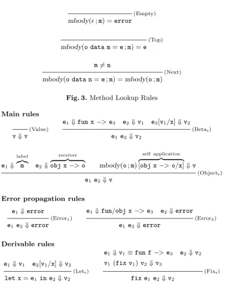
Fig. 3. Method Lookup Rules Main rules v+ v (Value) e1+ fun x > e3 e2+ v1 e3[v1/x]+ v2 e1 e2+ v2 (Betav) e1+ label z}|{ m e2+ receiver z }| { obj x > o mbody(o ; m) self application z }| { [obj x > o/x]+ v e1 e2+ v (Objectv)
Error propagation rules e1+ error e1 e2+ error (Error1) e1+ fun/obj x > e3 e2 + error e1 e2+ error (Error2) Derivable rules e1+ v1 e2[v1/x]+ v2 let x= e1 in e2+ v2 (Letv) e1+ v1⌘ fun f > e3 e2+ v2 v1(fix v1) v2+ v3 fix e1 e2+ v2 (Fixv)
Fig. 4. Big Step Operational Semantics (We let v6⌘ error)
Lookup algorithm. The lookup algorithm is defined in Figure 3. Intuitively:
– (Empty) If we didn’t find the method m after reading the whole method list, we’re “shouting” an error.
– (Top) If we find the method m then we have reach a goal, and we just need to return the body of the method.
– (Next) If this is not the method m, we are going to check elsewhere.
Again, inheritance is out of the scope of this paper, but it would not be difficult to add an object-based inheritance.
2.3 Big Step Natural Operational Semantics
We continue with a (call-by-value) big-step operational semantics on closed terms in Figure 2.2. The big-step semantics is self-explaining and immediately suggests how to build an interpreter for our calculus.
2.4 Type System
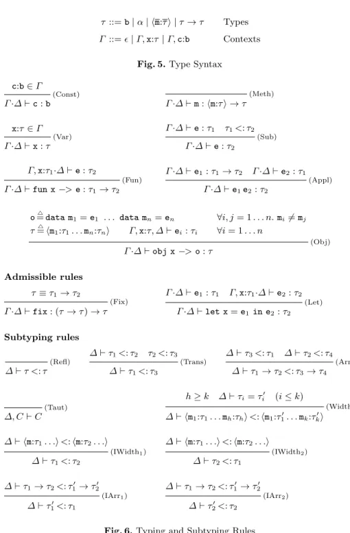
⌧ ::= b| ↵ | hm:⌧i | ⌧ ! ⌧ Types ::= ✏| , x:⌧ | , c:b Contexts
Fig. 5. Type Syntax c:b2 · ` c : b (Const) · ` m : hm:⌧i ! ⌧ (Meth) x:⌧2 · ` x : ⌧ (Var) · ` e : ⌧ 1 ⌧1<: ⌧2 · ` e : ⌧2 (Sub) , x:⌧1· ` e : ⌧2 · ` fun x > e : ⌧1! ⌧2 (Fun) · ` e 1: ⌧1! ⌧2 · ` e2: ⌧1 · ` e1e2: ⌧2 (Appl)
o= data m4 1= e1 . . . data mn= en 8i, j = 1 . . . n. mi6= mj
⌧=4hm1:⌧1. . . mn:⌧ni , x:⌧, ` ei: ⌧i 8i = 1 . . . n · ` obj x > o : ⌧ (Obj) Admissible rules ⌧⌘ ⌧1! ⌧2 · ` fix : (⌧ ! ⌧) ! ⌧ (Fix) · ` e 1: ⌧1 , x:⌧1· ` e2: ⌧2 · ` let x = e1 in e2: ⌧2 (Let) Subtyping rules ` ⌧ <: ⌧ (Refl) ` ⌧ 1<: ⌧2 ⌧2<: ⌧3 ` ⌧1<: ⌧3 (Trans) ` ⌧ 3<: ⌧1 ` ⌧2<: ⌧4 ` ⌧1! ⌧2<: ⌧3! ⌧4 (Arr) , C` C (Taut) h k ` ⌧i= ⌧i0 (i k) ` hm1:⌧1. . . mh:⌧hi <: hm1:⌧10. . . mk:⌧k0i (Width) ` hm:⌧1. . .i <: hm:⌧2. . .i ` ⌧1<: ⌧2 (IWidth1) ` hm:⌧1. . .i <: hm:⌧2. . .i ` ⌧2<: ⌧1 (IWidth2) ` ⌧1! ⌧2<: ⌧10 ! ⌧20 ` ⌧10<: ⌧1 (IArr1) ` ⌧1! ⌧2<: ⌧10 ! ⌧20 ` ⌧20<: ⌧2 (IArr2)
Fig. 6. Typing and Subtyping Rules
– b are just the basic types, while ↵, , . . . are type variables.
– hm:⌧i is a set of (di↵erents) method names with types. More formally it is a row of the form hm1:⌧1 . . . mn:⌧ni, for some n 0.
– contexts records the types of constants and of the free-variables.
Typing rules. The typing and subtyping rules are introduced in Figure 6. A brief explanation follows for the (sub)typing rules: We introduce a second context which contains constraints of the form
– ↵ <: ⌧ where ⌧ is either an object, a variable or a constant type. Basically anything but arrows but in a more general context, anything where subtyping is not defined recursively.
– ⌧ <: ↵ where ⌧ is either an object, a variable or a constant type.
The reason for the restriction on the constraints in is that the other kind of constraints can be broken down into smaller ones, or they are trivially unsolvable. However, allowing any constraint to appear in does not seem to be much of a complication, and the metatheory seems to be mostly independent from this choice.
– ` ⌧1= ⌧2 means ` ⌧1<: ⌧2 and ` ⌧2<: ⌧2
– (Const, Var) Nothing surprising here, these are usual rules for constants and variables. – (Meth) This is the key rule: since methods are to be used as functions, they have to be typed
as functions. They get here their natural type: if you give a method m an object with a method m of type ⌧ then it returns an expression of type ⌧ . Note that the type requires object with only m as a method, however subtyping allows you to use an object with any other methods. – (Fun, Appl) These are usual rules.
– (Obj) The type of an object is a row, where each method is given the type of its body in a enriched context that takes into account the type of the object itself (represented by x). – (Sub) The subsumption rule means that if e has a type ⌧ , then e has any supertype of ⌧ too.
e.g.: ` obj x > data m = fun x >x data n = fun x > fun y > x y : hm:↵ ! ↵i because of (Sub) rule.
– For the admissible rules:
• (Fix) Monomorphic type for the fix point combinator. This is usual, yet confusing. It basically means that you can only do a fix point of a term shaped as fun f > fun x > e. • (Let) A usual monomorphic typing rule for let.
– (Refl, Trans, Arr) These are the common rules when working with subtyping. (Refl) and (Trans) are the rule that enforce <: to be a preorder. (Arr) is a structural rule which describes how the super-terms are behaving in regards of <: .
– (Taut) This rules allows the constraints in the context to be understood by the typing system. It’s the only rule which “reads” , basically assuming that what says is true.
– (Width) This is the base case of the subtyping order. An object can “forget” some of its methods (i.e. the methods he remember must keep the same type though). To understand why depth subtyping is not possible see [AC96]. Note that since there is no inheritance, the present system could have accepted some covariant depth subtyping; since we want the system to be ready for upgrade with inheritance, we actually drop this feature.
– (IWidthi) these two rules invert the property of the width subtyping. The . . . in it mean “any
other methods with any type” They don’t need to be the same in both objects.
Usually inverting the rules can, of course, be done by an induction on the derivation of the subtyping judgement. Unfortunately, with the addition of constraints, we can’t always do it without these rules. For example
=hm:↵i <: , <: hm: i
Then, we can derive ` hm:↵i <: hm: i but it’s not true that ` ↵ = . Which is unsound, even though is a perfectly reasonable constraint context.
– (IArri) these two rules invert the property of the arrow subtyping. The idea is much the same
as in (IWidth). An example of a which would require it would be: =hm:↵1! ↵2i <: , <: hm: 1! 2i
We have ` ↵1! ↵2<: 1! 2 thanks to the (IWidth1) rule. But not ` 1<: ↵1 if we
3
Metatheory
This section introduces the metatheory of our calculus. Soundness and completeness of the big-step semantic w.r.t. the small-big-step one basically ensure that both semantics do essentially the same thing.
Theorem 1 (Soundness and Completeness of ! w.r.t. +). 1. (Soundness) If e1+ v and v 6= error, then e !! v.
2. (Completeness) If e1!! v, then the big step converges, i.e. there exists v0 such that e+ v0.
Proof. 1. (Soundness) Straightforward induction on the derivation of e1+ v.
2. (Completeness) This part can be proved via Melli`es’s standardization lemma [Mel96]. Definition 1.
A constraint context is said flat if all the constraint it contains are of the form: b1<: b2
Definition 2.
A constraint context is said consistent if: – = 1, 2 and 1 is flat
– there exists a substitution such that, for all C2 2 1` C
Lemma 1 (Substitution in Subtyping).
Let be a consistent constraint context, and a substitution such that for all C 2 , 0 ` C
for some constraint context 0. If ` ⌧
1<: ⌧2 then 0 ` ⌧1 <: ⌧2 .
Proof. Straightforward induction on the derivation of ` ⌧1<: ⌧2.
Lemma 2 (Subtyping Without Inversion).
We call a derivation without inversion of ` ⌧1<: ⌧2any such derivation which does not use any
of the rules (IWidthi) or (IArri). Here is a list of proprieties of such derivation. Let 1 be a flat
constraint context.
1. If 1` ⌧1! ⌧2<: ⌧0 is derivable without inversion, then ⌧0 ⌘ ⌧10 ! ⌧20 and 1 ` ⌧10<: ⌧1 and 1` ⌧2<: ⌧20 are derivable without inversion.
2. If 1 ` hm1:⌧1. . . mh:⌧hi <: ⌧0 is derivable without inversion, then ⌧0 ⌘ hm1:⌧10. . . mk:⌧k0i with
h k and 1` ⌧i<: ⌧i0 and 1` ⌧i0<: ⌧i are derivable without inversion for each 1 i h.
3. If 1` ⌧ <: ⌧0 is derivable, then it is also derivable without inversion.
Proof.
1. Straightforward induction on the derivation without inversion of 1` ⌧1! ⌧2<: ⌧0.
2. Straightforward induction on the derivation without inversion of 1 ` hm1:⌧1. . . mh:⌧hi <: ⌧0
(remember that 1 is flat, thus does not contain any constraint involving such types).
3. By induction on the derivation of 1 ` ⌧ <: ⌧0, all cases are straightforward, except the
inversion ones which are resolved simply by applying the previous two results. This is a small useful lemma for the proof of the following.
Lemma 3 (Subtyping). Let be a consistent context.
1. If ` hm1:⌧1. . . mh:⌧hi <: h. . .i where h. . .i is any object type, then h. . .i ⌘ hm1:⌧10. . . mk:⌧k0i with
h k with ` ⌧i = ⌧i0 for all 1 i k.
Proof. 1. Since is consistent, there exist a such that = 1, 2 with 1 flat, and for all
C2 2 1` C . It is obvious then, that for all C 2 , 1` C .
Then we have, applying Lemma 1 (Substitution in Subtyping), that 1` hm1:⌧1. . . mh:⌧hi <: h. . .i .
Hence h. . .i ⌘ hm1:⌧100. . . mk:⌧k00i for some k h (by Lemma 2, Subtyping Without Inversion).
It obviously means that h. . .i ⌘ hm1:⌧10. . . mk:⌧k0i. Then we conclude because (IWidthi) ensure
This lemma states that you can specialize (i.e. replace a type by a subtype) any type in the environment, and still be able to derive the same types.
Lemma 4 (Specialization).
If , x:⌧1· ` e : ⌧ and ` ⌧2<: ⌧1 then , x:⌧2· ` e : ⌧.
Proof. By induction on the derivation of , x:⌧1· ` e : ⌧:
– (Var) Either e⌘ y 6⌘ x and this is straightforward. Either e ⌘ x and ⌧ ⌘ ⌧1, then:
, x:⌧2· ` x : ⌧2 (Var)
` ⌧2<: ⌧1
, x:⌧2· ` x : ⌧1
(Sub)
– The other cases are straightforward.
This is the most important lemma in order to prove Subject Reduction theorem. Lemma 5 (Generation).
1. If · ` x : ⌧ then there exists ⌧0 such that x:⌧02 and ` ⌧0<: ⌧ .
2. If · ` m : ⌧ then there exists ⌧0 such that · ` m : hm:⌧0i ! ⌧0 and ` hm:⌧0i ! ⌧0<: ⌧
3. If · ` fun x > e : ⌧ then there exists ⌧1, ⌧2 such that ` ⌧1! ⌧2<: ⌧ and , x:⌧1· `
e: ⌧2. Moreover, if ⌧ ⌘ ⌧10 ! ⌧20 then , x:⌧10· ` e : ⌧20.
4. If · ` obj x > o : ⌧ then there exists ⌧i with i = 0 . . . n such that ⌧0 ⌘ hm1:⌧1. . . mn:⌧ni
and , x:⌧0· ` mbody(o ; mi) : ⌧i for all i = 1 . . . n and · ` obj x > o : ⌧0and ` ⌧0<: ⌧
5. If · ` e1 e2: ⌧ then there exists ⌧1 such that · ` e1: ⌧1! ⌧ and · ` e2: ⌧1.
Proof. 1. Straightforward induction on the derivation of · ` x : ⌧ (there are only two cases: (Var) and (Sub) ).
2. Straightforward induction on the derivation of · ` m : ⌧: (again, there are only two cases (Meth) and (Sub) ).
3. Induction on the derivation of · ` fun x > e : ⌧. (Fun) Obvious.
(Sub) By induction hypothesis (let’s note the previous type ⌧0 with ` ⌧0<: ⌧ ) we have that
there exists ⌧1 and ⌧2 such that ` ⌧1! ⌧2<: ⌧0 and , x:⌧1· ` e : ⌧2.
Then, by transitivity, ` ⌧1 ! ⌧2<: ⌧ moreover, if ⌧ ⌘ ⌧10 ! ⌧20 we have that `
⌧0
1<: ⌧1, by Lemma 4 (Specialization), we have that , x:⌧10· ` e : ⌧2. We also have that
` ⌧2<: ⌧20, by the subsumption rule, we have the result.
4. Straightforward induction on the derivation of · ` obj x > o : ⌧. 5. Straightforward induction on the derivation of · ` e1 e2: ⌧ .
This is the usual Substitution Lemma, it is crucial to prove Subject Reduction. Lemma 6 (Substitution).
If , x:⌧1· ` e1: ⌧ and · ` e2:⌧1 then · ` e1[e2/x] : ⌧ .
Proof. Straightforward induction on the derivation of , x:⌧1` e1: ⌧ .
Theorem 2 (Subject Reduction).
If is consistent, · ` e1: ⌧ , and e1! e2, then · ` e2: ⌧
(Callv) Because of Lemma 10, we have that · ` m : ⌧1! ⌧ and · ` obj self > o : ⌧1.
Also there exists ⌧0 such that · ` m : hm:⌧0i ! ⌧0 and ` hm:⌧0i ! ⌧0<: ⌧1 ! ⌧. And ⌧i0
with i = 0 . . . n such that ⌧00 ⌘ hm1:⌧10. . . mn:⌧n0i and , self:⌧00· ` mbody(o ; mi) : ⌧i0 for all
i = 1 . . . n and · ` obj self > o : ⌧0
0 and ` ⌧00<: ⌧1.
Then, we can derive :
` ⌧0 0<: ⌧1 ` hm:⌧0i ! ⌧0<: ⌧1! ⌧ ` ⌧1<:hm:⌧0i (IArr1) ` ⌧0 0<:hm:⌧0i (Trans)
Now, we apply Lemma 3 (Subtyping), and we get that one of the mi is actually m and that
` ⌧i= ⌧0. Hence the result (using Lemma 6 (Substitution), and the fact that ⌧0<: ⌧ ).
Lemma 7 (Progress).
Let be a consistent constraint context.
1. If · ` e : ⌧, then the evaluation of e cannot produce error, i.e. e 6!! C[error] for every context C[·].
2. If· ` e1: ⌧ then, either e1 is a value, or there exists e2 such that e1 ! e2.
Proof. 1. Direct corollary for Theorem 2 (Subject Reduction), since error has no type.
2. Straightforward proof by induction on the typing derivation. We also need usual extension of Lemma 3 (Subtyping) to ensure that arrows types and object types are inhabited only by function and objects respectively (or looping expression. Remember that we are in an empty type context, meaning that e1 is closed.
4
Principal Typing
We will now be interested in the property of principal typing. The goal of this section is two present an algorithm to infer a principal constrainted type.
Definition 3 (Principal Constrainted Type). A principal constrainted type of e under · is a pair ( 0, ⌧ ). Such that:
– 0is realisable by meaning that there exists a substitution such that for all C2 0, ` C .
– · , 0` e : ⌧.
– For all ⌧0 such that · ` e : ⌧0 there exists a substitution with ⌧0= ⌧ and for all C2 0,
` 0 .
All substitution refered in this definition are supposed to leave invariant ( i.e. = ) Note that by Lemma 1, the two last points are converse to each other. The first point means that objects with no type have no principal constrainted type either.
In the following we will be interested mainly in inference where is empty. The extension to non-empty is costless in term of decidability as long as the subtyping relation entailed by is decidable. An usual example of non-empty context would be a flat context, with such a context, complexity either should not be an issue.
We can build an inference algorithm in the following fashion: i( ; ; x) = (⌧ <: ↵; ↵) where x:⌧ 2
i( ; ; e1 e2) = ( 0, 00, ⌧0<: ⌧00 >↵; ↵) where i( ; ; e1) = ( 0; ⌧0)^ i( ; ; e2) = ( 00; ⌧00)
i( ; ; fun x > e) = ( , ↵! ⌧ <: ; ) where i( , x:↵; ; e) = ( 0; ⌧ ) i( ; ; m) = (hm: i ! <: ↵; ↵)
Where all the variables introduced are fresh.
Note that this algorithm only has variable types as output, which ensures that the constraint set it engenders is a constraint context.
It is not difficult to see that i( ; ; e) verifies both two last points of the definition of principal constrainted type. Now of course, since this algorithm always terminates with a solution, and there are indeed untyped terms, we need to discriminate which are principal constrainted types for e and which are actual untyped terms. This reduces, when is empty to the satisfiability of constraints which is known to be decidable in polynomial time for this kind of subtyping relation [Pot98].
This is achieved roughly by saturating the constraint set with all possible derivable contraints and represent all the constraints in a graph.
We now know that we can find a principal typing for any typable expression in OhML or answering that no type is available when none is. Still, this type is presented as a cluster of constraints which are to be applied to a type variable. This is barely readable, but there are ways to make it clearer. One can hope benefiting from the constraint solving algorithm to get a smaller constraint set, also when a variable ↵ appears in a type ⌧ only in covariant positions, and if ↵ has an greatest lower bound derivable from the constraint context, then, it is safe to substitute ↵ with its greatest lower bound in ⌧ . Respectively if ↵ appears only in contravariant positions and have a least upper bound.
5
Examples
This section shows some type assignments for some interesting programs. The purpose of this section is to drive the reader to the next, more formal section, with a clear intuition of the inference algorithm.
5.1 Heating up
Those examples show some simple inferences in suitable constraint contexts. ;· <: ↵ ` fun x >(n x)(m x) : hn:↵ > , m: i >
;·↵ <: hm: i ` fun x >fun y >x y; m y : (↵ > ) >↵ >
;·hm: > i <: ↵ ` fun x >fun y >x y; x (obj >data m = fun x >x) : (↵ > ) >↵ > ;· <: ↵, <: ` fun x >fun y >x (y x)(y x) : (↵ > > ) >((↵ > > ) > ) > ;·↵ <: hn: i ` fun x > (n (m x)) : hm:↵i >
5.2 Find the Principal Type: a Manual Run
The following example shows how the algorithm is able to generate all constraints and finally find the principal type (it it exist).
Take the following function:
fun x >fun y >x (y x) 1. First of all we have =4x:↵, y: ;
2. Then we try to infer some type for x (yx) and we fold all the constraints, i.e. <: ↵ > and ↵ <: > ;
3. Then, we simplify the constraints, i.e. 1 > 2<: ↵ > and ↵1 >↵2<: > , i.e.
<: ↵1
↵2<:
↵ <: 1 2<:
4. By transitivity, on could again simplify: we add ↵1 >↵2<: 1;
5. By constraint rewriting, we simplifiy again: we substitute ↵1 >↵2<: 1 for 11<: ↵1, et
↵2<: 12;
6. We can build a , by taking all the created constraints (of course trivial equality constraint are dropped, e.g.
4
= 2<: , <: ↵1, ↵2<: , 11<: ↵1, ↵2<: 12
7. Now, we get =4x:↵1 >↵2, y:( 11 > 12) > 2;
8. We fix the typing derivation as follows:
;· ` fun x >fun y >x (y x) : (↵1 >↵2) >(( 11 > 12) > 2) >
9. We minimize by replacing all type variables in covariant position with their lower bound, and al contravariant position with their upper bound, i.e.
min4=;
10. Finally, the inferred judgment will be:
;·; ` fun x >fun y >x (y x) : (↵1 >↵2) >((↵1 >↵2) >↵1) >↵1
6
Adding Inheritance
We will now show how inheritance can be featured in OhML. It is well known that inheritance and subtyping do not mix well (see for instance [Liq97]). In a first attempt we will implement inheritance in a “dynamic update” style, meaning that we can override methods in objects to create new ones, but not to add new method names.
This method of inheritance can appear weaker but it has been shown [AC94] that it allows encoding of usual class-based inheritance. Being able to add new method names to an object can still be an improvement to our system, but in the presence of an expression based and functional calculus, our first attempts have been disrupted, showing an unexpected number of difficulties.
This extension however, is rather straightforward, and can easily be understood from the inheritance-free calculus.
Let’s add an inheritance operator to the syntax of objects: o::= ✏| compose e | o data m = e
We have now two types of objects. The basic ones allowing defining new signatures, and the composed ones inheriting from another object. We will enforce the new methods of composed objects to have the same name as some method of the inherited object with the type system.
But first, we need to update the semantics of objects. We will first give the new definition of values:
v::= ⌫| fun x > e | obj x > ! | error ! ::= ✏| compose obj x > ! | ! data m = e
The idea behind this new value definition, is that we’ll need to reduce the composed object to ensure that the lookup algorithm makes any sense at all.
Let us give the new rule of the lookup for composition (for simplicity purpose, we suppose the objects from which it is inherited to have been ↵-renamed to have the same self name):
mbody(! ; m) = e
mbody(compose obj x > ! ; m) = e
(Inherit)
And the updated rule for (Callv)-reduction:
This is a simple tweaking dealing with the need of reduction inside composition.
The type syntax stays the same and all prior typing and subtyping rules still holds. We only need an extra rule for composed object to type. This rule will allow us to ensure that the created object has no extra method names:
o=4compose e0 data m1= e1 . . . data mn= en 8i, j = 1 . . . n. mi6= mj
· ` e0: ⌧ ⌧4=hm1:⌧1. . . mn:⌧ni , x:⌧, ` ei: ⌧i 8i = 1 . . . n
· ` obj x > o : ⌧
(Obj)
Note by the way that by this definition, we consider the self name unbound in the compose expression.
The metatheory of this new calculus is a straightforward extension of the earlier one, the intuition behind this extension behind rather clear. We won’t state it here but the same results hold.
7
Adding polymorphism
The system has been designed until now without polymorhpic let. But adding it is not an difficult issue. We just have to take care of the fact that we have constraints. The idea is simple, it comes clear from the syntax of type schemes:
s::=8↵. .⌧
A type scheme has to contain all the constraint needed over its variables to ensure safe instancia-tion. For instance consider:
e= fun x > obj > compose x data m = e1 data n= e2
If· ` e1: ⌧1 and· ` e2: ⌧2, then the type scheme
8↵.↵ <: hm:⌧1, n:⌧2i.↵ ! ↵
Is a scheme which entails all the types of e provided ⌧1 and ⌧2being unique types.
To carry the intuition into the type system, let us define a generation and instanciation oper-ator:
Gen( ; , 0; ⌧ ) = ( ;8↵. 0.⌧ ) if ↵\FTV( ) = ;^↵\FTV( ) = ;^8C 2 0. ↵\FTV(C) 6= ;
Inst( ;8↵. 0.⌧ ) ={⌧ | 8 62 ↵. = ^ 8C 2 0. ` C }
These two operator are a constrainted extension of those in more usual ML-like type systems. They give the needed typing rules straightforwardly. We need to change the variable rule:
⌧2 Inst( ; s) , x:s· ` x:⌧ (Var) · 0` e 1: ⌧1 ( ; s)=4Gen( ; 0; ⌧1) , x:s· ` e2: ⌧2 · ` let x = e1 in e2: ⌧2 (Let)
8
Type inference algorithm
Type inference in presence of subtyping is a delicate problem: in the last ten years a lot of re-searchers have studied this topic on various forms and techniques (for a good survey we refers to the Pottier’s Ph.D. thesis [Pot98], or its Habilitation thesis [Pot04], or the course note of Leroy-Pottier [LP]). The Mitchell’s paper [Mit91] on Type Inference With Simple Subtypes has shown that adding subtyping with subsumption rule in a simple type system complicates the inference algorithm. This means that solving the equation system is a non trivial problem especially in presence of function-types (that behave contravariantly in the function argument) and in presence of non atomic types, like e.g. object-types. Mitchell’s paper designed a type inference algorithm, calledG. In our OhML calculus, the presence of objects and object-types complicate the inference. The algorithmAlg presented in this paper is inspired and an extension of Mitchell’s one.
Prerequisites. The following definition sets up the semantic structure of constraint set used by an inference algorithm.
Definition 4 (The constraint-set C).
1. A constraint-set of subtyping equations is inductively defined as follows: C ::= ; | C [ {⌧ <: ⌧}
2. A subtyping statement ⌧1<: ⌧2 is provable in C, if ⌧1<: ⌧2 can be proved using the subtyping
in C plus the rules of Figure 6. (⌧1<: ⌧2 could be also be written asC ` ⌧1<: ⌧2.)
3. We writeC1` C2 if C1` ⌧1<: ⌧2 for all ⌧1<: ⌧22 C2.
4. (Transitivity) IfC1` C2, andC2` C3, thenC1` C3.
The algorithm. In what follows we present a type inference algorithm, called Alg, conceived as an extension of the Mitchell’sG algorithm; that is, given an untyped term, Alg produces a triple (C, , ⌧), such that ` e : ⌧ (in a given C), or fails. The set C, usually called constraint-set, contains the subtyping assertions that must be satisfied in order the type judgment ` e : ⌧ being derivable. It is worthy noticing that the presentation of the type system of Figure 6 omits the setC in the premises of the judgment, i.e. ` e : ⌧ should be intended as C · ` e : ⌧. Definition 5 (The Algorithm Alg).
The algorithm Alg is given via an inference system presented in Figure 10; it uses the classi-cal algorithm mgu, that is the unification algorithm between first-order terms of [Rob65] (hence omitted).
A brief explication of the algorithm follows:
– (rAConst), (rAVar) Those two rules are axioms that gives the most general context satisfying the subtyping constraints for constants and variables.
– (rAMeth) This rule is an axiom for method inference; it just set a suitable constraint-set. – (rAAbs1), (rAAbs2) Those two rules deal with abstraction; the main di↵erence is that the in
former rule the variable x occurs in e, while in the latter not. Suitable constraint-sets and type-contexts are built.
– (rAAppl) This rule (directly inherited fromG), deals with function/method application/invocation: two constraint-setsC1, andC2are built together with two contexts 1, and 2, and two inferred
types ⌧1, and ⌧2for e1 and e2, respectively. An hygiene condition on the free type-variable of
⌧1and ⌧2is required. If there exists a substitution ✓, most general unifier between the common
variables in contexts 1 and 2, and unifying the domain of the arrow-type of e1 with the
inferred type of e2, then a new merged constraint-set, a new merged type context, and an
All ↵ type-variables are considered fresh.They can be indexed. Alg(c) = ({b1<: b2} ; c:b1; b2) (rAConst) Alg(x) = ({↵1<: ↵2} ; x:↵1; ↵2) (rAVar) Alg(m) = ({hm:↵1i ! ↵1<: ↵2} ; ; ; ↵2) (rAMeth) Alg(e) = (C ; ; ⌧1) 9⌧2. x:⌧22 Alg(fun x > e) = (C [ {⌧2! ⌧1<: ↵1! ↵2} ; \ {x} ; ↵1! ↵2) (rAAbs1) Alg(e) = (C ; ; ⌧1) @⌧2. x:⌧22 Alg(fun x > e) = (C [ {↵3! ⌧1<: ↵1! ↵2} ; ; ↵1! ↵2) (rAAbs2) Alg(e1) = (C1; 1; ⌧1) Alg(e2) = (C2; 2; ⌧2) Ftv(⌧1)\ Ftv(⌧2) =; 9✓ = mgu({ 1(x) ? = 2(x)| 8x. x 2 Dom( 1)\ Dom( 2)} [ {⌧1 ? = ⌧2! ↵1}) Alg(e1 e2) = (C1✓[ C2✓[ {↵1✓ <: ↵2} ; 1✓, 2✓ ; ↵2) (rAAppl)
o= data m4 1= e1 . . . data mn= en Ti=1...nFtv(⌧i0! ⌧i00) =;
Alg(fun x > ei) = (Ci; i; ⌧i0! ⌧i00) 8i = 1 . . . n
9✓ = mgu { i(y)
?
= j(y)| 8y. y 2 Dom( i)Ti,j=1...nDom( j)}
S i=1...n{hm1:⌧100. . . mn:⌧n00i ? = ⌧0 i} ! Alg(obj x > o) = (Si=1...nCi✓ S i=1...n{⌧i0✓ <: ↵1} ;Si=1...n i✓\ {x} ; ↵1) (rAObj)
Fig. 7. The Type Inference Algorithm
– (rAObj) This rule deals with objects. Given an object with n methods, first we calculate n-triples of (constraint-set;context;inferred-type). An hygiene condition on the free type-variables of all the inferred arrow-types is required. If there exists a substitution ✓, most general unifier between all the common variables in contexts i, with i = 1 . . . n, and unifying all the
arrow-types of fun x > ei, with i = 1 . . . n, where x is the type of the full object (i.e. the type
of this), then a new merged constraint-set, a new merged type context, and an inferred type is given.
Example 1 (A run ofAlg). Consider the term e4
=fun y > obj x > data m = y. Let 4
=y:↵1, and let:
C1 =4 {↵1<: ↵2} C2 4= {↵3! ↵2<: ↵4! ↵5} C3 =4 {hm:↵5i <: ↵6} C4 4= {↵1! ↵6<: ↵7! ↵8} Alg(y) = (C1; ; ↵2) Alg(fun x >y) = (C1[ C2; ; ↵4! ↵5) 9✓ = [hm:↵5i/↵4]. mgu({hm:↵5i ? = ↵4}) Alg(obj x > data m = y) = (C1✓[ C2✓[ C3✓ ; ✓ ; ↵7! ↵8) Alg(e) = (C1✓[ C2✓[ C3✓[ C4;; ; ↵7! ↵8)
given the expression e, its principal typing is found by finding a minnum set C5 such thatC1✓[
C2✓[ C3✓[ C4 ` C5. This is usually done by using a term rewriting system that “propagates”
from left-to-right all the minimum-type constraints until a single (singleton) constraint-set of the form{⌧1<: ⌧2} is obtained. Constraints between arrow-types are decomposed as usual, i.e. {⌧1!
⌧2<: ⌧3! ⌧4} {⌧3<: ⌧1} [ {⌧3<: ⌧4}. Constraints between object-types are decomposed
point-wise, i.e. {hm1:⌧1. . . mn:⌧ni <: hm1:⌧1. . . mn:⌧n0i} Si=1...n{⌧i<: ⌧i0}. If this rewriting terminates,
then, the type ⌧1 is the principal type of e. Pragmatically.
C1✓[ C2✓[ C3✓[ C4 (C2✓[ C3✓[ C4)[↵1/↵2] ⌘ {↵3! ↵1<:hm:↵5i ! ↵5} [ C3[ C4 ⌘ {hm:↵5i <: ↵3, ↵1<: ↵5} [ C3[ C4 (C3[ C4)[hm:↵5i/↵3, ↵1/↵5]⌘ {hm1:↵1i <: ↵6} [ C4 C4[hm1:↵1i/↵6]⌘ {↵1! hm1:↵1i | {z } principal type <: ↵7! ↵8} ⌘ C5
Then the principal type of e exists and it is ↵1! hm1:↵1i for some ↵1.
Lemma 8 (Soundness and Completeness of mgu). (Soundness) If mgu(C) = ✓, then ✓ is a solution for C.
(Completeness) If # is a solution for C, then mgu(C) = ✓ such that ✓ # (where ✓ # () 9 . # = ✓).
Theorem 3 (Soundness and Completeness of Alg).
1. (Soundness) IfAlg(e) = (C ; ; ⌧), and C {⌧1<: ⌧2}, then ` e : ⌧1, and ⌧ ⌧1.
2. (Completeness) Suppose 2` e : ⌧2. ThenAlg(e) = (C1; 1; ⌧1), and C1 C2 ⌘ {⌧1<: ⌧3}.
Then 1 2 and ⌧1 ⌧2. ( is the usual preorder).
Proof. The proof from Mitchell paper seem to fit this adaptation well; it relies in propagate and simplify constraints; it is quite technical and it is currently being checked. A bit of care must be devoted in studying complexity of the algorithm.
9
Conclusions and future work
We introduced a functional calculus `a la Curry that features uniformly message sending and function application in a simple and natural way. The type system is rather simple, just function-types, record-types and subtyping to deals with functional fix points (fix points are not really essential to the first-class method label encoding). The system is proved to prevents message-not-found run-time errors. We also adapt of the Mitchell’sG type inference algorithm [Mit91]. There are a few propositions of such things in the literature, such as Bugliesi-Crafa [BC99], or M¨ uller-Nishimura [MN00]. Besides using a rather richer language (featuring first-class functions), we the think that our proposition is extremely simple since it does not need extreme complication neither in the type system nor in the source language.
Among the possible further work we would like to mention those few items: – study the complexity ofAlg.
– improve OhML with an object-based inheritance. – add polymorphic-types and polymorphic type-inference. – add references and reference-type.
Acknowledgments. The authors are sincerely grateful to Fran¸cois Pottier and Didier Remy, for the fruitful discussions on type inference with subtyping and for suggesting a further simplification of the core OhML calculus. We also warmly thank all the anonymous referees of a previous submission for their insight comments and sharp suggestions that helped us to improve the paper. This work is supported by the French grant CNRS ACI Modulogic.
References
[AC94] Martin Abadi and Luca Cardelli. A Theory of Primitive Objects: untyped and first order systems. In Proc. of TACS, volume 789 of Lecture Notes in Computer Science, pages 296–320. Springer-Verlag, 1994.
[AC96] M. Abadi and L. Cardelli. A Theory of Objects. Springer-Verlag, 1996.
[BC99] M. Bugliesi and S. Crafa. Object calculi with dynamic messages. In FOOL’6 Workshop on Foundation of Object Oriented Languages, 1999.
[DM82] L. Damas and R. Milner. Principal Type-Schemes for Functional Programs. In Proc. of POPL, pages 207–212. The ACM Press, 1982.
[FHM94] K. Fisher, F. Honsell, and J. C. Mitchell. A Lambda Calculus of Objects and Method Special-ization. Nordic Journal of Computing, 1(1):3–37, 1994.
[Liq97] L. Liquori. Bounded Polymorphism for Extensible Object. Technical Re-port CS-24-96, Computer Science Department, University of Turin, Italy, 1997. ftp://lambda.di.unito.it/pub/liquori/bounded97.ps.
[LP] X. Leroy and F. Pottier. Course DEA: Typage et programmation. http://pauillac.inria.fr/ ~fpottier/mpri/dea-typage.ps.gz.
[Mel96] P-A Melli`es. Description Abstraite des Syst`emes de R´e´ecriture. PhD thesis, Universit´e Paris 7, December 1996.
[Mit91] J. C. Mitchell. Type inference with simple subtypes. In Journal of Functional Programming, 1991.
[MN00] M. M¨uller and S. Nishimura. Type inference for first-class messages with feature constraints. International Journal of Foundations of Computer Science, 11(1):29–63, 2000.
[Pot98] F. Pottier. Synth`ese de types en pr´esence de sous-typage: de la th´eorie `a la pratique. PhD thesis, Universit´e Paris 7, July 1998.
[Pot04] F Pottier. Types et Contraintes. M´emoire d’habilitation `a diriger des recherches, Universit´e Paris 7, 2004.
[Rob65] J.A. Robinson. A machine-oriented logic based on the resolution principle. Journal of the ACM, 12(1):23–49, 1965.