Assessing the climate resilience of buildings to the effects of hygrothermal loads: impacts of wind-driven rain calculation methods on the moisture performance of massive timber walls

(1)

https://doi.org/10.4224/40001821

Vous avez des questions? Nous pouvons vous aider. Pour communiquer directement avec un auteur, consultez la

première page de la revue dans laquelle son article a été publié afin de trouver ses coordonnées. Si vous n’arrivez pas à les repérer, communiquez avec nous à PublicationsArchive-ArchivesPublications@nrc-cnrc.gc.ca.

Questions? Contact the NRC Publications Archive team at

PublicationsArchive-ArchivesPublications@nrc-cnrc.gc.ca. If you wish to email the authors directly, please see the first page of the publication for their contact information.

https://publications-cnrc.canada.ca/fra/droits

L’accès à ce site Web et l’utilisation de son contenu sont assujettis aux conditions présentées dans le site LISEZ CES CONDITIONS ATTENTIVEMENT AVANT D’UTILISER CE SITE WEB.

READ THESE TERMS AND CONDITIONS CAREFULLY BEFORE USING THIS WEBSITE.

https://nrc-publications.canada.ca/eng/copyright

NRC Publications Archive Record / Notice des Archives des publications du CNRC : https://nrc-publications.canada.ca/eng/view/object/?id=28872b4c-5440-4a1f-bb35-9148ab70e8f6 https://publications-cnrc.canada.ca/fra/voir/objet/?id=28872b4c-5440-4a1f-bb35-9148ab70e8f6

NRC Publications Archive

Archives des publications du CNRC

For the publisher’s version, please access the DOI link below./ Pour consulter la version de l’éditeur, utilisez le lien DOI ci-dessous.

Access and use of this website and the material on it are subject to the Terms and Conditions set forth at

Assessing the climate resilience of buildings to the effects of

hygrothermal loads: impacts of wind-driven rain calculation methods

on the moisture performance of massive timber walls

(2)

Assessing the Climate

Resilience of Buildings to the

Effects of Hygrothermal Loads

Impacts of Wind-driven Rain Calculation

Methods on the Moisture Performance of

Massive Timber Walls

Author(s): M. Defo, M.A. Lacasse and N. Snell

Report No.: CRB-CPI-Y3-R06

Report Date: 30 April 2019

Contract No.: A1-012820-13

Agreement Date: 29 November 2016

CONSTRUCTION

(3)

(4)

List of Figures

Figure 1. Typical measured rain admittance factors (RAF) for simple buildings (Straube & Burnett, 2000; Straube, 2010) ... 8 Figure 2. Comparison of temperature, total annual rain, relative humidity and wind speed during the time period 1986-2016 in Calgary, Ottawa and Vancouver. ...12 Figure 3. Comparison of the hourly rain distribution for the two years selected for simulation in Ottawa (1989/2004), Vancouver (2009/2007) and Calgary (1995/2012). The first and second years in each case are the year with the median and maximum moisture index, respectively. Day 0 corresponds to January 1st of the first year. ...12 Figure 4. Configuration of a CLT exterior wall assembly for Cold climates (adapted from Karacabeyli & Lum (2014)). ...13 Figure 5. Typical exterior CLT wall assembly configurations (Nordic, 2015) ...14 Figure 6. Geometry of the 1-D configuration of the CLT exterior wall used for simulation ...19 Figure 7. Air-field wind-driven rain rose for the two years of simulation for Calgary, Ottawa, and Vancouver ...19 Figure 8. Comparison of the vapour permeability and the thermal conductivity of the two insulation materials used in the wall systems considered ...20 Figure 9. Spatial discretization of a massive timber wall (case of wall W2 with 128 mm insulation) ...22 Figure 10. Comparison of the total WDR over the two years of simulation obtained with SB, ASHRAE and ISO WDR calculation methods ...24 Figure 11. Comparison of WDR distribution over two years of simulation obtained with SB, ASHRAE and ISO WDR calculation methods for the city of Ottawa. Y-axis scale was limited to 0 to 20 to permit visualization of lower intensity rain events. ...27 Figure 12. Comparison of WDR distribution over two years of simulation obtained with SB, ASHRAE and ISO WDR calculation methods for the city of Vancouver. ...28 Figure 13. Comparison of WDR distribution over two years of simulation obtained with SB, ASHRAE and ISO WDR calculation methods for the city of Calgary. Y-axis scale was limited to 0 to 20 to permit visualization of lower intensity rain events. ...29 Figure 14. Comparison of temperature of outer layer of CLT obtained with SB, ASHRAE and ISO WDR calculation methods. ...30 Figure 15. Comparison of relative humidity of outer layer of CLT obtained with SB, ASHRAE and ISO WDR calculation methods. ...32 Figure 16. Comparison of relative humidity of outer layer of CLT panel obtained with SB, ASHRAE and ISO WDR calculation methods under Calgary climate conditions. Assumption that 1% of WDR penetrates wall and is uniformly distributed on outer surface of sheathing membrane. ...33 Figure 17. Comparison of relative humidity of outer layer of CLT panel obtained with SB, ASHRAE and ISO WDR calculation methods under climate conditions of Ottawa. Assumption that 1% WDR penetrates wall and is uniformly distributed on outer surface of sheathing membrane. ...35 Figure 18. Comparison of relative humidity of outer layer of CLT panel obtained with SB, ASHRAE and ISO WDR calculation methods under climate conditions of Vancouver.

(7)

Assumption that 1% of WDR penetrates wall and is uniformly distributed on outer surface of sheathing membrane. ...36 Figure 19. Mould index on outer layer of CLT panel obtained with SB, ASHRAE, and ISO methods under specified local climate conditions. Mould growth observed only with assumption of 1% WDR penetration for wall W1 at 30 and 50 m under climate conditions of Ottawa, and walls W1 and W2 at 30 and 50 m heights and for wall W3 at 10, 30 (not shown) and 50 m heights under climate conditions of Vancouver ...38

(8)

List of Tables

Table 1. ISO obstruction factor, O. ... 6

Table 2. ISO wall factor, W ... 7

Table 3. Parameters of the ISO roughness coefficient ... 7

Table 4. Exponent for different wind exposures (Straube, 2010) ... 9

Table 5. ASHRAE exposure factor, FE ...10

Table 6. Location & climate characteristics of 3 cities selected for hygrothermal simulations ....11

Table 7. Basic properties of materials used in walls W1, W2, and W3 ...20

Table 8. Parameters used to compute the WDR for SB, ASHRAE and ISO models in Terrain Category IV (urban areas) ...21

Table 9. Detail on meshing of different layers of wall with minimum & maximum element size ..23

(9)

(10)

Executive Summary

Water penetration in the wall assembly through deficiencies, resulting from the coupled action of rain and wind, also known as wind-driven rain (WDR), can cause degradation of tall wood building components (e.g. mould growth, wood decay), thereby by reducing their performance and service life. Three semi-empirical models are available in the literature to estimate the quantity of wind-driven rain that impinges on the cladding surface: the ASHRAE model, the ISO model, and the Straube and Burnett model (SB model). The objective of this work was to compare the consistency of the hygrothermal responses and the moisture performance of the CLT panel used in massive timber walls as predicted by hygrothermal simulations with WDR calculated using the three models. Three Canadian cities having contrasting climates were selected for simulation: Vancouver (BC) located in Climate Zone 5 with a minimum RSI-value requirement of 3.60; Ottawa (ON) located in Climate Zone 6 with a minimum RSI-value requirement of 4.053; and Calgary (AB) located in Climate Zone 7A with a minimum RSI-value requirement of 4.76. Three massive timber wall systems that differ by their insulation type and thickness were considered: a wall having 2 layers of 89 mm mineral fibre insulation with RSI-value of 5.7 (W1); a wall having two layers of 64 mm mineral fibre insulation with RSI-RSI-value of 4.4 (W2); and a wall having a sprayed polyurethane foam insulation of 89 mm with RSI-value of 4.5 (W3). As well three building heights (10, 30 and 50 m) were tested. Due to RSI-value restriction, only wall W1 was considered in Calgary. For Ottawa and Vancouver, all the three walls were considered as they all meet the minimum R-value requirements. In each city, simulations were run using DELPHIN v5.9.4 for two years as selected from a historical climate data set based on the moisture index. For this study, only the fibreboard cladding was considered. The wall orientation receiving the most WDR over the two-year period was selected for simulations in each city, assuming that the building is located in city centre. Material properties were taken from the NRC material property database. Water penetration in the structure was assumed to be 1% of the wind-driven rain as recommended by the ASHRAE Standard 160. Temperature and relative humidity of the outer layer of the CLT panel were compared amongst the three WDR calculation models. The mould growth index on the outer layer of the CLT panel was used to compare the moisture performance predicted using respective models.

WDR calculated by the three methods differed by city and building height but in general the ASHRAE and the SB models gave similar results, which are higher than the ones obtained with the ISO model. The difference between the results obtained with ASHRAE and SB models on one side, and that obtained with the ISO model on another side were much higher in Vancouver than in Ottawa and Calgary, and increased with increasing height of the building.

Temperature profiles of the outer layer of the CLT panel were all in good agreement for the three models in the three cities and for all the insulation types and building heights considered. The results for relative humidity differed with respect to whether or not the water infiltration in the structure is assumed, the insulation type and the building height. With the assumption of no water infiltration, all the three methods of calculating WDR gave the same results with respect to the relative humidity of the outer layer of the CLT in all cities and for all insulation types and

(11)

building heights. When it was considered that 1% WDR penetrates in the structure, differences in relative humidity of the outer layer of the CLT were found amongst the three models. The SB model generally gave higher relative humidity values for the outer layer of the CLT panel, which were relatively close to those obtained by the ASHRAE model. However, for some walls, a difference of up to 10% was found between the SB and ASHRAE models. The results obtained with these two models were consistently higher than those obtained by the ISO model. The differences between the results obtained with ASHRAE and SB models on one side and the ISO model on another side varied with city and building heights, reflecting the results of WDR calculations. Differences were negligible in Calgary, but significant in Ottawa and Vancouver. The largest differences (about 20%) in relative humidity were found in Vancouver for the three wall systems and for the heights of 30 and 50 m.

With respect to mould growth risk, conditions for temperature and relative humidity of the outer layer of the CLT panel obtained with the ISO model were unfavourable to the mould growth for all three cities and for all wall systems and building heights. Both SB and ASHRAE models predicted no significant mould growth on the outer layer of the CLT panel in Calgary for W1 at all heights, in Ottawa for W1 and W2 at all heights and W3 at 10 m, and in Vancouver for W1 and W2 at 10 m and 30 m. In Ottawa for W3 at 30 and 50 m, SB model predicted higher mould risk than ASHRAE model. In Vancouver for wall W1 and W2 at 50 m, SB model predicted significant mould risk while ASHRAE model predicted no mould risk. For W3 in Vancouver at 10 m, SB model predicted higher mould risk while ASHRAE predicted no mould growth at all. For the same wall at 30 and 50 m, SB and ASHRAE models predicted similar high mould risk. For the cases analyzed, the three methods consistently showed the same trend in terms of moisture performance: the SB method predicts the highest risk; the ASHRAE method predicts either smaller or similar risk compared to SB method; and the ISO method predicts the lowest risk. This means either of the three models can be used for comparative studies. However, since both SB and ASHRAE methods give the most conservative results, each of the two methods could be used for addressing the climate resiliency and the durability of tall wood building envelopes. It would be recommended to proceed with the same type of analysis for other types of wind exposures (open country and suburban areas) where the wind patterns are different than for the city center and that can lead to different results for wind-driven rain calculated by the three different models. As well, other cladding types could be tested.

(12)

Assessing the Climate Resilience of Buildings

to the Effects of Hygrothermal Loads

Impacts of Wind-Driven Rain Calculation Method on the

Moisture Performance of Massive Timber Walls

by

M. Defo, M. A. Lacasse and N. Snell

1 Introduction

Mass timber products are increasingly used in mid-rise and high-rise buildings, thanks to: (i) advanced wood technologies and modern mass timber products such as glued-laminated timber, cross-laminated timber (CLT), nail-laminated timber and structural composite lumber; (ii) NRCan’s Tall Wood Building Demonstration Initiative (2013-2017) whose goal was to foster commercial and regulatory uptake of tall wood buildings in Canada and the ongoing NRCan’s Green Construction through Wood (GCWood) Program1; (iii) provincial government initiatives (e.g. Ontario’s Tall Wood Building Reference2, Ontario Mass Timber Program3, The Wood Charter in Quebec4). Considerable efforts have been invested in developing technical data to support their implementation in North America (Gagnon & Pirvu, 2011; Karacabeyli & Lum, 2014). However, the primary emphasis has been placed on assessing structural, fire, and acoustical performance. Whilst many mass timber buildings have been or are being constructed in many jurisdictions across the country (e.g. Brock Commons Tallwood at UBC, Origine Tallwood building in Quebec City, etc.), there are still concerns about the thermal and hygrothermal response and expected moisture performance of mass timber products. Climate change notwithstanding, Tall Wood buildings are subjected to increased wind and rain loads given increases in building height. This prolongs the exposure of building enclosures to wind-driven rain and wind loads, and increases the risk of premature deterioration of wood-based wall and roof assemblies. It is also anticipated that future projections of the effects of climate change and extreme weather events will exacerbate the situation.

The current (2015) edition of the NBC includes climatic design data up to year 2006 and historical long-term data for the extreme events are not included in the code. Therefore, there is a need: (i) to update the current design climatic data of the NBC to include the historical climate data up to the current time, and (ii) to develop new climatic design data for future climate change scenarios. On the basis of the projected climate loads, the hygrothermal response of Tall Wood building enclosures will be assessed and analyzed.

1 https://www.nrcan.gc.ca/forests/federal-programs/gcwood/20046 2 https://www.omfpoa.com/wp-content/uploads/2017/11/Ontarios-Tall-Wood-Building-Reference-2017.pdf 3 https://www.ontario.ca/page/building-with-wood 4 https://mffp.gouv.qc.ca/english/publications/forest/wood-charter.pdf

(13)

In this context, in January 2018, NRC-CRC initiated the project ‘’Ontario Climate Resilient Tall wood Buildings and Structures’’. The overall objective of this project was to evaluate the effects of current historical climate loads and extreme climate events and those arising in the future from climate change on the thermal and hygrothermal response and durability of massive timber building products (MTP) used as enclosure components and assemblies for Tall Wood buildings, for a selected set of cities located in Ontario. During the winter 2018, A Scoping Study (Defo et al., 2018a) and Preliminary hygrothermal simulation tests (Defo et al. 2018b) were realized. Phase 2 of the project was thereafter planned in which was included:

 Characterization of CLT and NLT material properties;

 Laboratory testing on the effects of wind and rain loads (intensity, frequency, etc.) on CLT and NLT wall assemblies; benchmarking of hygrothermal model

 Laboratory testing on the thermal performance of CLT and NLT wall assemblies; benchmarking of thermal model;

 Hygrothermal simulation to determine the thermal and hygrothermal response of selected wall configurations to a range of climates loads, including loads as may arise due to the effects of climate change, for geographic locations in Ontario of interest to the client;  Whole building energy simulation for geographic locations in Ontario of interest to the

client.

Given the importance of the subject, the BRMA Program agreed to fund this initiative under the CRB-CPI project. However, the scope of the project was reduced and goals aligned to those of the CRB-CPI project, with focus on massive timber buildings across all the country.

Early in the spring 2018, six (6) pieces of 3S-105 CLT wood timber panels having dimensions of 8-ft. x 8-ft. were purchased for the purpose of building CLT wall assemblies on which to undertake the various laboratory tests. With the reduced budget, it was then decided to continue investigations on material properties of different wood species used in the manufacturing of CLT with focus on determining the absorption (suction) and drainage curve to characterise the absorption-desorption isotherms that were acquired during the first phase of the project. This will permit obtaining the full hysteresis loop and analysis of the impact of hysteresis on the hygrothermal simulation results. These tests are still ongoing. It was also decided to submit a CLT panel alone under the gradient of temperature and relative humidity in the EEEF test facility to gather some data that can be used for benchmarking of simulation tools. Here too, the test is still ongoing.

During the initial phase of the project, preliminary simulation tests showed that wind-driven rain (WDR), especially the small fraction of the WDR that penetrates into the wall, has a greater impact on the hygrothermal simulation results. Given that the research community has not agreed on any method to calculate WDR, there was a need to redirect research on this topic so as to facilitate selection of a method that will be used in the subsequent phases of the project. As such and as other tasks were not completed, this report focuses on the work done to address the wind-driven rain calculation issue.

(14)

Water penetration in the wall assembly through deficiencies, resulting from the coupled action of rain and wind, also known as WDR, can cause deterioration of building components (e.g. mould growth, wood decay, corrosion of metallic fasteners, etc.); thereby by reducing their performance and service life. WDR is also an essential boundary condition for hygrothermal simulation. Therefore, the determination of the quantity of WDR is an important consideration for durable building envelope design. Three methods are typically used: (a) field measurements method; (b) semi-empirical method; and (c) numerical simulations based on Computational Fluid Dynamic (CFD) modelling.

A thorough review of field WDR measurements is provided by Blocken & Carmeliet (2004). They are performed to measure directly the quantity of WDR that reach the surface of the wall. Data obtained are also used to determine the coefficients of semi-empirical models. However, this method can be expensive, time-consuming and limited to specific buildings and locations. A more detailed distribution of WDR on façades can be provided by Computational Fluid Dynamics (CFD) modelling. This numerical method was developed by Choi (1993), updated and validated by Blocken & Carmeliet (2002), and extensively described by Blocken & Carmeliet (2002, 2004), Blocken et al. (2007) and Kubilay et al. (2013). CFD simulation is regarded as the most accurate method to calculate the quantity of WDR that arrives at the surface of the wall. Any type of building can be modelled. The results are the spatial distribution of the WDR on the facades, a function of horizontal rainfall intensity, wind speed and wind direction. Shortcomings to this method are their complexity that limits their practical use, their expensive costs and their time consumption (Blocken & Carmeliet, 2004). This method cannot be used in a large-scale study that implies consideration of many different types of buildings and locations.

The limitations of field measurements and CFD simulations have led researchers to develop semi-empirical models based on relationships between the amount of WDR and the influencing meteorological parameters such as horizontal rain fall, wind velocity, wind direction, wall orientation, etc. These methods provide rough estimation of WDR that are easy to use, and are based on formulas that can be applied to many building geometries and locations. Nowadays, the most frequently used semi-empirical models are: the International Organization for Standardization (ISO) Standard for WDR assessment (International Organization for Standardization, 2009) (ISO model), the model developed by Straube and Burnett (Straube & Burnett, 2000) (SB model) and the model from the American Society of Heating, Refrigerating and Air-Conditioning Engineers (ASHRAE) Standard 160-2016 (ASHRAE, 2016) (ASHRAE model). These three models will be used in this comparative study. They will be detailed in Section 2.1.

Many studies on WDR were dedicated on the benchmarking of different semi-empirical models using field measurements or comparing WDR models. Nath et al. (2015) measured WDR loads on building facades in three Canadian cities (Fredericton, Montreal and Vancouver) and compared with WDR calculated using the ISO model. Because wind velocity and rain were measured on-site, all the factors in the model were set to 1. The preliminary results show that the ISO model overestimates the WDR amount most of the time. A similar study by Ge et al. (2018) using high resolution weather data led to the same conclusions that ISO model

(15)

overestimates wall factor and therefore WDR loads. Wind-driven rain estimation on a cubic building using CFD-catch ratio model was found to be 18-38% greater than that using the

semi-empirical models ISO and ASHRAE in three Canadian cities (Ge, 2015). The ISO and SB

models were compared based on their influencing parameters for the four terrain categories defined in ISO (Blocken & Carmeliet, 2010). It was found that in the two semi-empirical models, the values of the wall factor W (for ISO) and the rain admittance factor RAF (for SB), which have the same definition in both models, can differ more than a factor 2 from each other and can therefore provide very different WDR results. Moreover, the authors showed that the ISO and SB models behave almost the same for terrain category II with regards to the roughness coefficient used to correct for the increasing wind velocity with the height in the ISO model, and the wind speed correction factor in the SB model, but differently for other terrain categories. For example, for terrain category III and IV, the roughness coefficient in the ISO model decreases while the wind speed correction factor increases in the SB model. This will result with higher WDR amount calculated using the SB model. Blocken et al. (2010) compared the ISO model, the SB model and the CFD model by applying them to four idealised buildings under steady-state conditions of wind and rain. They showed that the ISO model incorrectly provides WDR coefficients that are independent of horizontal rain, while the SB model shows a dependency that is opposite to that by CFD. In addition, the SB model can provide very large overestimations of the WDR deposition fluxes at the top and side edges of buildings (up to more than a factor 5).

2 Objectives

To our knowledge, none of the studies that dealt with the evaluation of different WDR calculation methods has extended the investigation to their impacts on moisture performance of walls. As consequence, there is no information that can guide on the selection of a proper WDR model to address the impacts of climate change on the durability of massive timber walls. This study was designed to fill this gap. The main objectives are to:

(1) Compare the three semi-empirical WDR calculation models, namely ASHRAE, ISO and SB models, with respect to consistency of hygrothermal responses obtained under different climate conditions and for different massive timber building heights.

(2) Assess the degree to which the difference in hygrothermal responses might lead to different conclusions to the risk of premature degradation of wall components.

(3) Select a suitable method to be used for CRB-CPI project.

3 Methods

Three typical massive timber walls were selected for comparing the moisture performance using three semi-empirical WDR calculation methods (SB, ASHRAE and ISO methods). They differ by their insulation type (i.e. mineral fibre and polyurethane foam) and thickness (i.e. 89 mm for polyurethane, 128 mm and 178 mm for mineral fibre); a description of the common elements of the wall assembly is given in §2.4. Three (3) Canadian cities characterized by their much-contrasted climates were chosen (i.e. Ottawa, Vancouver, and Calgary) for locations of simulation; the climate characteristics for each of these locations is given in §2.3. Simulations

(16)

were run over a period of two (2) years using the DELPHIN heat, air and moisture simulation tool. Only a one-dimensional configuration of the wall was simulated. Comparisons were made using relative humidity and temperature of the outer surface of the CLT panel, and the risk of mould development on the outer surface of the CLT panel. It was assumed that the wall was perfectly air tight and that 1% of WDR penetrates in the structure through deficiencies and reached the surface of the sheathing membrane. In the following sections, details and considerations are provided of the various parameters needed for simulations and the evaluation of risk to premature degradation of the respective wall assemblies.

3.1 Review of semi-empirical WDR calculation methods

The semi-empirical models were developed on the basis of Lacy’s equation describing the intensity of the free WDR (the driving rain that is not affected by the building or other obstructions). Under the assumptions that all raindrops are of the same size and that the wind flow is uniform, steady, horizontal and perpendicular at all the times to the vertical surface, the intensity of WDR passing through a the vertical plane can be expressed as (Hoppestad, 1955; Korsgaard, 1962; Lacy, 1965) cited by Blocken & Carmeliet (2004):

= ℎ . (1)

Where: Rwdr is the rainfall intensity received on a vertical surface (mm/h); Rh is the rainfall

intensity received on a horizontal surface (mm/h); U is the horizontal component of the wind speed (m/s); and Vtis the rain drop’s terminal velocity (m/s). The terminal velocity is a function

of the raindrop size, which is a function of the horizontal rainfall intensity (Best, 1950). Using the median rain drop size, Lacy (1965) refined Eq. (1) relating wind speed and rainfall intensity to driving rain:

= . . ℎ (2)

Where: α is the WDR coefficient (s/m), the inverse of the raindrop’s terminal velocity. Lacy reported a value of α = 0.222 s/m, which corresponds to an average spell composed of similar rain drop diameter of 1.2 mm, with a terminal velocity of 4.5 m/s. Eq. (2) is a measure of the free WDR since it assumes no deflection of wind or raindrops by the vertical plane. To calculate the amount of driving rain on an actual facade, both wind and building parameters need to be considered. Therefore, the wind speed at a specific location has to be adjusted by taking into account the effect of terrain, local topography, obstruction factors as well as the height of the building. The wind flow changes pattern when it approaches the actual building, which results in the deposition of raindrops carried by wind to certain areas of the building (Ge, 2015). The three semi-empirical models (SB, ASHRAE, and ISO) derived from Eq. (2). They differ from each other in terms of the driving-rain coefficient and correction factors.

3.1.1 ISO model

The ISO standard 15627-3 (ISO, 2009), derived from the British Standard BS 8104 (BSI, 1992), provides a procedure to calculate the WDR incident on a wall based on a long series

(17)

measurements of driving rain on buildings in a wide range of locations within the UK (Blocken & Carmeliet, 2010). The resulting equation is given by:

= . _ℎ⁄ . �. �. . . � (3)

Where: U10 is the hourly average airfield wind speed at 10 m from the ground (m/s), Rh is the

total hourly horizontal rainfall intensity (mm/h), θ is the angle in the horizontal plane between the wind direction and the normal to the façade; CT is the topography coefficient taking into account

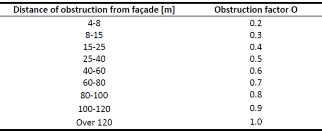
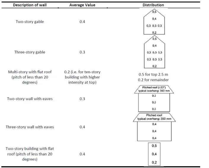
the increase in mean wind speed over isolated hills and escarpments, this value ranging from 1 for upstream slopes of less than 5% inclination to 1.6 for buildings located on steep hills; O is the obstruction factor that considers the shelter caused by the nearest obstacle of similar dimensions as the wall (Table 1); W is the wall factor that takes into account the variation of the rain deposition amount on different areas of the facade (Table 2); and CR is the terrain

roughness coefficient that considers the variability of mean wind velocity at the site due to the height above the ground and the roughness of the terrain in the direction from which the wind is blowing. Wall factors provided in the ISO standard are for a limited number of building geometries, mainly low-rise buildings; these factors are restricted to only a few values for the entire façade without taking into account differences over the width and height of the façade. The terrain roughness coefficient CR is calculated using equations (4) and (5):

� � = �. (_{� ) for z z}� i (4)

� � = � � � for z < z i (5)

Table 1. ISO obstruction factor, O (ASHRAE, 2016).

(18)

Table 2. ISO wall factor, W (ASHRAE, 2016)

Table 3. Parameters of the ISO roughness coefficient (ASHRAE, 2016)

3.1.2 Straube-Burnett (SB) model

The semi-empirical model developed by Straube and Burnett (2000), transforms the driving-rain from free-field to the specific location on the façade by introducing the ‘Rain Admittance Factor’ (RAF), as given in Eq. (6):

(19)

= �. ��. . ℎ. � (6) Where: Uz is the wind speed (m/s) at the height of interest z (m); θ is the angle between the

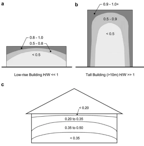
normal to the wall and the wind direction (o); DRF is the driven rain factor and RAF is the rain admittance factor. The RAF makes the conversion of the free-field WDR intensity to the WDR intensity on the building façade. The authors provided some values of the RAF in graphical form for three types of building geometries (Figure 1).

Figure 1. Typical measured rain admittance factors (RAF) for simple buildings (Straube & Burnett, 2000; Straube, 2010)

The Driven-Rain Factor (DRF) is the inverse of the raindrop terminal velocity:

� = (7)

In the SB model, the terminal velocity of raindrops (Vt) is computed from the equation developed

by Dingle and Lee (1972):

(20)

Where: d is the raindrop diameter (mm). Straube and Burnett (2000) found a good correlation between the measured and calculated values of DRF using the median raindrop diameter as estimated by the cumulative probability distribution of raindrop diameters proposed by Best (1950):

� = − � {− _.

ℎ. .

} (9)

Where: F(d) is the cumulative probability distribution of raindrop diameters for a given rainfall intensity; d is the equivalent spherical raindrop diameter (mm); and Rh is the rainfall intensity on

a horizontal plane (mm/m2/h). The median raindrop diameter is defined by (Best 1950):

= . × . × ℎ . (10)

Where: n = 2.25. Based on the information provided in literature and results from their own experiments, Straube and Burnett (2000) found that the value of the DRF varies between 0.2 and 0.25 for average conditions, but can differ significantly for different rainfall intensities and type of events. For instance, the DRF ranges from more than 0.5 for drizzle to 0.1 for intense cloudbursts. The wind velocity at any height Uz, can be calculated from Eq. (11) as suggested

Straube (2010):

= . � � (11)

Where: U10 is the standard wind speed at 10 m above grade (m/s), z is the height above grade

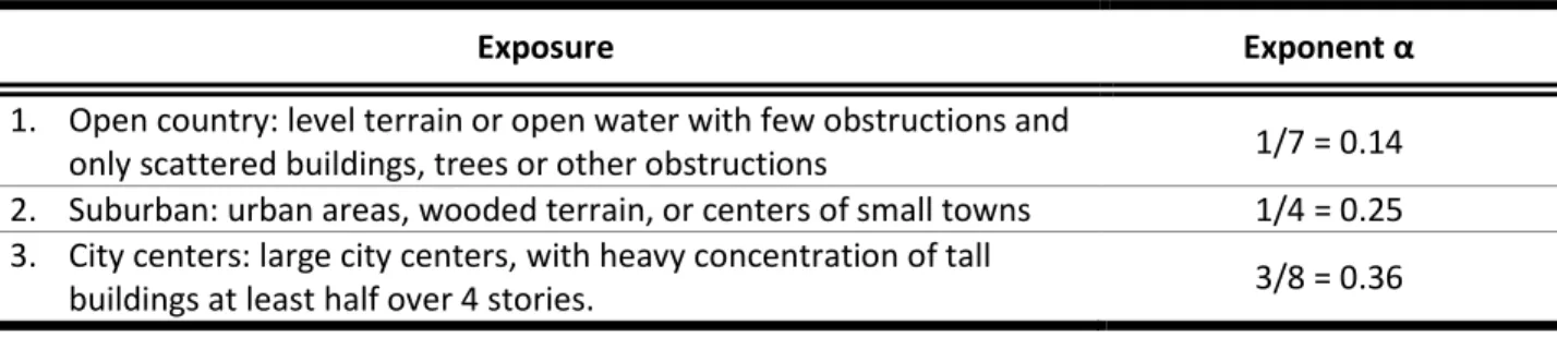
(m) and α is the exposure exponent that depend on the type of wind exposure of the building (Table 4).

Strictly speaking, and as suggested by Blocken and Carmeliet (2010), the SB model should be used only for the terrain category where weather station is located since there is no factor to transform the wind speed measured in one terrain category to another.

Table 4. Exponent for different wind exposures (Straube, 2010)

Exposure Exponent α

1. Open country: level terrain or open water with few obstructions and

only scattered buildings, trees or other obstructions 1/7 = 0.14 2. Suburban: urban areas, wooded terrain, or centers of small towns 1/4 = 0.25 3. City centers: large city centers, with heavy concentration of tall

buildings at least half over 4 stories. 3/8 = 0.36

3.1.3 ASHRAE model

(21)

= � . � . ��. . �. ℎ (12) Where: FE is the rain exposure factor, depending on the building height, the terrain topography

and the surroundings; FD is the rain deposition factor accounting for the spatial distribution of the

WDR on the façade; FL is an empirical constant (= 0.2 kg·s/(m3.mm)); U10 is the hourly mean

wind velocity at 10 m; θ is the angle between the normal to the wall and the wind direction; and

Rh is the rain intensity on the horizontal surface (mm/h).

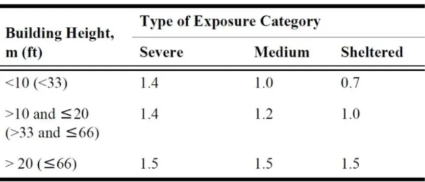
In the ASHRAE model, the exposure factor FE is equivalent to the combined effect of CR and CT as given in the ISO model. As shown in Table 5, three categories of exposure factors are suggested, given for different building heights and terrain types: severe, medium and sheltered. Severe exposure includes hilltops, coastal areas, and funneled wind (e.g. wind tunnel effect caused by the proximity of two buildings). Sheltered exposure includes protection from nearby buildings or other permanent moderating features (e.g. trees). The rain deposition factor, FD, is

equivalent to the wall factor W in the ISO standard and RAF in SB model. Whereas in the ISO standard six situations to determine the wall factor are provided (Table 2), only three situations are given in the ASHRAE standard: 0.35 for walls below a steep-slope roof, 0.5 for walls below a low-slope roof and 1.0 for walls subject to rain runoff.

Table 5. ASHRAE exposure factor, FE

3.2 Geographical locations

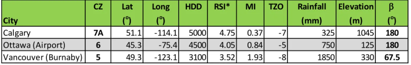
Three (3) Canadian cities of contrasting climate were selected for this study; these included: Ottawa (ON), Vancouver (BC), and Calgary (AB). Their location and respective climate characteristics are provided in Table 6. The moisture index (MI) and Heating Degree-Days (HDD), reported in the 2015 edition of National Building Code, are 1.93 and 3100, 0.84 and 4500, and 0.37 and 5000, respectively, for Vancouver, Ottawa and Calgary. The reason for selecting these locations of different climate severity was to verify if the hygrothermal responses and the performance of the wall obtained using different methods of calculating the WDR loads and indoor condition loads may vary with the climate type.

(22)

Table 6. Location & climate characteristics of 3 cities selected for hygrothermal simulations

3.3 Climate data

The historical climate data (1980-2016) was sourced from the hourly and daily climate databases of Environment and Climate Change Canada. Missing values were filled-in using bias-corrected data from the Climate Forecast System Reanalysis (CFSR; Saha et al. 2010). To perform bias-corrections, multiplicative or additive (depending on the climate variable being corrected) correction factors (CFs) were calculated for each month and hour by comparing the CFSR data with observational data, and thereafter the CFs were applied to correct CFSR data. In respect to CFSR data for rainfall and snow-cover, biases in the number of wet or dry days were also corrected. The corrected CFSR data was then used to fill-in missing values in the observational database. The direct and diffuse radiation values were derived from global radiation values using the method of Orgill and Hollands (Orgill & Hollands, 1977).

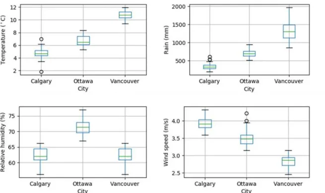
The difference in some of the climate variables amongst the three cities during the time period 1986-2016 are presented in Figure 2. It can be noted that the average temperature, average wind speed and annual rainfall are quite different amongst these three cities.

3.3.1 Selection of moisture reference years

Ideally, to assess the impacts of WDR on the performance of the wall, simulations should be run on the 31-year series of climate. However, this approach would be unpractical as it would require longer times to perform simulations. The common approach of assessing the hygrothermal performance of the wall is to use Moisture Reference Year(s) (MRYs) data for hygrothermal simulations (Cornick et al., 2003; Candenedo et al., 2006; Salonvaara et al., 2010). For undertaking hygrothermal simulations in this study, two representative years were selected from the historical climate data (1986-2016) of each city, based on the moisture index (MI) approach (Cornick et al., 2003). The first and second years were, respectively, the year with the median and that with the highest MI values of the 31-year data set. They correspond respectively to the years 1989 and 2004 for Ottawa, 2009 and 2007 for Vancouver, and 1995 and 2012 for Calgary.

CZ Lat Long HDD RSI* MI TZO Rainfall Elevation b

City (o) (o) (mm) (m) (o)

Calgary 7A 51.1 -114.1 5000 4.75 0.37 -7 325 1045 180

Ottawa (Airport) 6 45.3 -75.4 4500 4.05 0.84 -5 750 125 180

Vancouver (Burnaby) 5 49.3 -123.1 3100 3.52 1.93 -8 1850 330 67.5

CZ: Cl i ma te Zone; La t: La ti tude; Long: Longi tude; HDD: Hea ti ng Degree-da ys ; RSI* = Mi ni mum RSI-Va l ue; MI: Moi s ture i ndex; b: Wall orientation (from north)

(23)

Figure 3 compares the hourly rain data for the two years selected for simulations in the three cities. Vancouver is characterized by more rain events of lower intensity spread over the entire year whereas in Ottawa and Calgary, rain events are of greater intensity, being, for Ottawa, concentrated between April and November and, for Calgary, between June and September.

Figure 2. Comparison of the annual average temperature, relative humidity and wind speed, and total annual rain, during the time period 1986-2016 in Calgary, Ottawa and Vancouver.

Figure 3. Comparison of the hourly rain distribution for the two years selected for simulation in Ottawa (1989/2004), Vancouver (2009/2007) and Calgary (1995/2012). The first and second years in each case are the year with the median and maximum moisture index, respectively. Day 0 corresponds to

January 1st of the first year.

3.4 Wall assembly and building heights

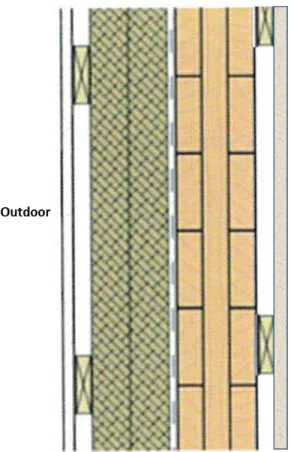
Massive timber wall assemblies are generally designed to ensure moisture durability, energy efficiency, fire safety, and noise control. In cold, heating dominated climate zones, exterior

(24)

insulation (Figure 4) is the preferred design approach (Gagnon & Pirvu, 2011; Karacabeyli & Lum, 2014). From exterior to interior, timber wall assemblies comprise the cladding, drainage cavity, insulation, air barrier/water resistive barrier, and CLT panel. The CLT panel is encapsulated in drywall for fire safety but where it is permitted, it can be left exposed.

Figure 4. Configuration of a CLT exterior wall assembly for Cold climates (adapted from Karacabeyli & Lum (2014)).

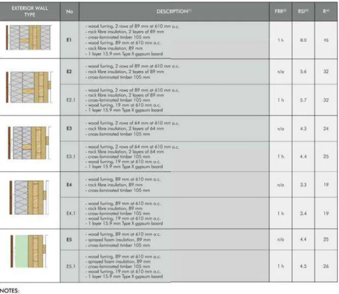
The use of a vapour permeable insulation is recommended to allow for outward drying of the CLT if initially wetted or if there is water penetration due to deficiencies. There is no need for vapour barrier since the CLT panel provides sufficient outward vapour resistance. The material and thickness of insulation depend on climate zone. Figure 5 shows some typical wall compositions suggested by Nordic (Nordic, 2015). For climate zones 5 (Vancouver), 6 (Ottawa), and 7A (Calgary), the minimum RSI-value as recommended by the National Energy Code for Buildings (NECB, 2015) is 3.60, 4.05 and 4.76 m2K/W, respectively. The type E2.1 (called W1 in the remainder of the report) was selected for Calgary. The types E2.1, E3.1 (called W2 in the remainder of the report) and E5.1 (called W3 in the remainder of the report) can accommodate the climate zone of Vancouver and Ottawa. They were therefore selected for these two locations.

Three building heights were considered for each wall: a 3-storey (10 m) low-rise building; a 10-storey (30 m) mid-rise building, and; a 17-10-storey (50 m) high-rise building. They are all have a flat roof. For this type of building, the intensity of rain deposition is higher at the top and edges

(25)

according to Straube and Burnett (2000). In this study, only the top area of each building will be considered. As such, in the remainder of the report, the three (3) buildings will be referred to in respect to their total heights (10 m, 30 m, and 50 m).

Figure 5. Typical exterior CLT wall assembly configurations (Nordic, 2015)

3.5 Hygrothermal simulations

3.5.1 Simulation tool

(26)

DELPHIN 5, v5.9.4, was used for hygrothermal simulations. The DELPHIN 5 (Coupled Heat, Air, Moisture and Pollutant Simulation in Building Envelope Systems) program was developed during 2004-2006 with funding support from research grants from the U.S. Environmental Protection Agency, U.S. Department of Energy, Syracuse Center of Excellence in Energy and Environmental Systems, EQS-STAR Center/New York State Office of Science, Technology and Academic Research, and Syracuse University5. It is maintained by the Institute for Building Climatology, Faculty of Architecture, Technical University of Dresden, Germany. It is intended for the coupled heat, air, moisture, and matter (salts, pollutants) transport in porous building materials. It can solve one and two-dimensional problems and has been successfully validated with HAMSTAD Benchmarks 1 through 5 (Sontag et al., 2013), and with experimental data (Langmans et al., 2012). The model uses either the full sorption isotherm or water retention function. Material properties are defined as function of volumetric moisture content and temperature. Climate data is entered as individual files for each climate variable. An important feature of DELPHIN is its ability to handle wind-driven rain deposition, and shortwave and longwave radiation as part of its boundary conditions, as well as air leakage, and moisture and heat sources.

Transport models

3.5.1.1

The governing equation for moisture transfer is given in Eq. (13) (Nicolai and Grunewald 2014): � �

� − ∇. [ ∇ + � ] − ∇. [ , �� (� )∇ ] − ∇. [ ∇ + � ] = (13)

Where: ρm is the total moisture (liquid + vapour + ice) density (kg/m3); Kl is the liquid conductivity

(s); Pl is the liquid pressure (Pa); Dv, air is the vapour diffusivity in air (m2/s); Rv is the gas

constant of water vapour (J/kgK); μ is the vapour diffusion resistance factor; g is the volume

fraction of gas (m3/m3); f(g) is a function of volume fraction of the gas; ρm is the liquid density

(kg/m3); cv is the vapour mass concentration (kg/kg); Kg is the air permeability (s); Pg is the gas

pressure; ρg is the humid air density (kg/m3); g is the gravity constant (m/s2); and Sm is the

moisture source or sink (kg/m3). The first, second, third, and fourth terms on the left hand side of Eq. (13) represent the accumulation of moisture, the mass flow of liquid, the diffusive flow of vapour, and the convective flow of vapour due to air movement, respectively.

The energy equation is given by Eq. (14) (Nicolai and Grunewald 2014): �

� − ∇. [ ∇ ] − ∇. [ ∇ ] − ∇. [ , �� (� )∇ ] − ∇. [ [ ∇ + � ]] = ℎ (14) Where: U is the internal energy density (J/m3); ul is the specific internal energy for the liquid

water (J/kg); Lv is the specific enthalpy of vapour (J/kg); ug is the specific internal energy of the

gas phase (J/kg); and Sh is the heat source or sink (J/m3). The first, second, third and fourth

terms on the left hand side of Eq. (14) describe the storage of internal energy, the heat transport

(27)

by conduction, the transport of sensible heat due to movement of liquid water by capillarity, the latent heat transport, and the transport of energy by the gases during convection, respectively. The air flow in building material is described by Eq. (15) (Nicolai and Grunewald 2014):

− [ ∇ + � ] = (15)

Where: cg is the air mass concentration in the gas phase (kg/kg), and Kg is the gas permeability

of the material (s).

Boundary conditions

3.5.1.2

(i) Moisture transfer

The boundary conditions for moisture flow are described by Eq. (16) for an indoor boundary and Eq. (17) for an outdoor boundary (Nicolai and Grunewald 2014):

,� = �( ,�− ,�) + , (16)

, = ( , − , ) + , + �� (17)

Where: is the moisture flux normal to the surface (kg/m2s); pvsurf is the vapour pressure on the

surface (Pa); pv is the vapour pressure of the ambient air (Pa); be is the surface film coefficient

for vapour transfer (kg/m2sPa); gv, conv is the mass flow rate of vapour at the boundary due to air

convection (kg/m2s) (Eq. 23); and grain is the wind driven rain (kg/m2s). The indices o and i refer

to outdoor and indoor. The vapour exchange coefficient can be input as a constant value or in form of equation that describes the variation of the coefficient with wind velocity.

DELPHIN proposes to enter WDR as imposed flux measured or calculated outside the software by any mean or to use DELPHIN’s WDR calculation model. In this last case, the user must provide as climate variables the horizontal rain flux, the wind direction and velocity, as well as the wall parameter such as the orientation and inclination.

(ii) Heat transfer

The boundary conditions for heat transfer at the outdoor surface is given by Eq. (18) (Nicolai and Grunewald 2014):

= + �� + , � + , + �, + + (18)

Where: qc is the convective component (W/m2); qrain is the enthalpy of rain (W/m2); qv, diff is the

enthalpy flow due to vapour exchange by convection at the surface (W/m2); qv, conv is the

enthalpy carried by vapour due to air flowing into or out of the wall (W/m2); qa,conv is the enthalpy

of convective air flux (W/m2); qsw is the shortwave radiation flux, (W/m2); and qlw the longwave

radiation flux (W/m2). Each of these components is described below.

(28)

= ( − ) (19) Where: c is the convective heat transfer coefficient (W/m2K); To is the outdoor temperature

(C); and Tsurf is the surface temperature (oC). The convective heat transfer coefficient can be

provided either as a constant value or in form of an equation taking into account the effect of wind velocity.

Enthalpy of rain

�� = �� (20)

Where: ul(T) is the internal energy of liquid water (J/kgK), function of temperature.

Heat transfer at the surface due to vapour convection

, � = ℎ ( , − , ) (21)

Where: hv is the specific enthalpy of vapour (J/kg), function of temperature.

Heat of vapour flowing by convection of air into or out of the structure

, = � , (22)

Where: uv is the specific internal energy of vapour (J/kg), function of the air temperature; and gv, conv is the mass of convective vapour flux carried by air into or out of the material (kg/m2s):

, = �, (23)

Where: cv is the mass contraction of vapour; and ga,conv is the flux of air into or out of the

structure (Eq. 30).

Enthalpy of convective air flowing into or out of the structure

�, = � � �, (24)

Where: ua is the specific internal energy of air (J/kg), function of the air temperature.

Shortwave radiation flux

= � (25)

Where:  is the shortwave absorption coefficient of the surface; and Isw is the shortwave

radiation normal to the surface. The user has the option to provide either the measured or calculated total shortwave normal to the surface, or the direct and diffuse horizontal shortwave radiations together with the wall factor (wall inclination and orientation) and the latitude and time zone of the location. In this last case, DELPHIN computes the total shortwave normal to the wall surface which includes the direct normal component, the diffuse normal component, and the total reflected component when the albedo of the ground surface is not zero.

(29)

Longwave radiation flux

DELPHIN proposes three methods of setting the longwave radiations; specifically the:

 Imposed longwave flux in case the longwave radiation flux has been calculated by the user

 Longwave components

= ( − � ) + ( − � ) (26)

Where: fsky is the sky radiation factor; is the atmospheric counter radiation (W/m2);  is the

Boltzmann constant (W/m2K4); fgrnd is the ground radiation factor; and is the ground

counter radiation (W/m2). If this option is selected, the user must provide the atmospheric counter radiation and the ground counter radiation as climate variables, as well as the wall inclination. The sky radiation factor is calculated by:

= ( � ) � (27)

Where: _� is the wall inclination; and � is the longwave emission coefficient of the wall surface. The ground radiation factor is calculated by:

= � ( � )

� + � −

₍₂₈₎

Where: � is the ground longwave emission coefficient.  The Boltzmann calculation

= �( − ) + �( − ) (29)

Where: Tsky is the sky temperature (K); and Tgrnd is the ground temperature (K). The sky

temperature and the ground temperature have to be provided as climate variables.

Any of the above components of the outdoor boundary conditions for heat transfer can be set for the indoor boundary conditions if relevant.

(iii) Boundary conditions for air flow in building materials

DELPHIN defines the boundary condition for air flow in building materials as:

�, = � − � (30)

Where: ga, conv is the flux of air at the boundary (kg/m2s); _� is the air exchange coefficient (s/m),

set to a high value (~1000 s/m); Pelem is the air pressure in the surface element (Pa); Pa is the

(30)

3.5.2 Wall geometry and orientation

Only a one-dimensional configuration passing through the insulation in the horizontal direction was analyzed as indicated in Figure 6. This configuration excludes the strappings/furring.

Figure 6. Geometry of the 1-D configuration of the CLT exterior wall used for simulation

Using the wind-driven rain rose (Figure 7) the wall orientation receiving the most wind-driven rain for the two years of simulations was selected. For the cities of Ottawa, Vancouver and Calgary, this was 180o, 67.5 o and 180o from North, respectively.

Figure 7. Wind-driven rain rose for the two years of simulation for Calgary, Ottawa, and Vancouver

3.5.3 Material properties

DELPHIN requires the following material properties: material porosity (capillary, effective, and at 80%), dry density, dry specific heat capacity, moisture storage or suction curve, thermal conductivity, moisture diffusivity or water conductivity, and vapour permeability or vapour diffusion resistance. All material properties were obtained from the NRC material property database (Kumaran et al. 2002). The basic properties of all materials are presented in Table 7.

(31)

A comparison of the vapour permeability and thermal conductivity of the two types of insulation materials used is provided in Figure 8. The vapour permeability of the mineral fibre is about two order of magnitude greater than that of the sprayed polyurethane foam.

Table 7. Basic properties of materials used in walls W1, W2, and W3

Figure 8. Comparison of the vapour permeability and the thermal conductivity of the two insulation materials used in the wall systems considered

3.5.4 Boundary conditions

Indoor conditions

3.5.4.1

Indoor ambient temperature and RH were set constant to 21oC and 50%, respectively, in each city. The indoor surface heat and water vapour transfer coefficients were set to 8 W/m2K and 5.9 x 10-8 s/m, respectively; no radiation exchange was assumed indoor.

Wind-driven rain calculation

3.5.4.2

WDR was calculated using the ISO, ASHRAE, and SB methods. Three different types of buildings located in urban area were considered in the simulation: a 3-storey, a 10-storey, and a 17-storey building with flat roof. For each building type, the area of the façade considered was the one which is likely to receive the most WDR according to Straube and Burnett (2000). For this type of building, the intensity of the rain deposition is higher at the top and side edges

Density Specific heat Thermal conductivity Porosity Thickness A

Wall component Material (kg/m3) (J/kgK) (W/mK) (m3/m3) (mm) (kg/m2s0.5)

Cladding Fibreboard 900 1880 0.120 0.579 10.5 0.0006

Drainage cavity Air layer 1.2 1214 0.151 - 19.0

AB/WRB 30 min Asphalt imprgnated paper 909 1256 0.159 0.973 0.2

Insulation Mineral fibre 11.5 840 0.043 0.999 1781_{, 128}2

Sprayed polyurethane foam 39.7 1470 0.023 0.115 893 CLT panel Spruce (3 layers) 400 1880 0.088 0.964 33; 31; 33

Adhesive layer (2) 400 1880 0.088 0.964 4; 4

Air cavity Air layer 1.2 1214 0.151 - 19.0

Interior sheathing Primed and painted gypsum 700 870 0.160 0.400 12.7

(32)

according to Straube and Burnett (2000). In this study, only the top area of each building was considered. Unlike the SB method which explicitly corrects the wind velocity with increasing height of interest, the ISO and ASHRAE methods implicitly take into account the effect of increasing height on wind velocity through the roughness coefficient (CR) and the exposure factor (FE), respectively. For the SB method, the wind velocity was corrected for the height using Eq. (11).

To be able to compare the three semi-empirical methods, assumptions should be carefully considered to permit obtaining the correct set of parameters for each model. The building was assumed to be located in terrain category IV, which according to ISO Standard, relates to urban areas (KR = 0.24, z0 = 1 and zmin = 16). The corresponding exposure category in the ASHRAE 160-2016 standard is that of a sheltered exposure (Table 5). The SB method corrects for the height using the wind exponent coefficient α equal to 0.36 (Eq. 11) for urban areas (Table 4). Table 8 represents the factors and coefficients taken into consideration to compute WDR for each method and at different heights.

Table 8. Parameters used to compute the WDR for SB, ASHRAE and ISO models in Terrain Category IV (urban areas)

To compute the rain drop terminal velocity in the SB model, the predominant rain drop diameter, i.e. the diameter of the drops which account for the greatest volume of water in the air, was used rather than the median rain drop diameter as suggested by Straube (2010). It was computed using Eq. (31) according to Best (1950):

= . ℎ . ( − ) (31)

Where n = 2.25.

Outdoor conditions

3.5.4.3

Hourly data of climate loads (temperature, RH, wind velocity, wind-driven rain, shortwave and longwave radiations) on the exterior surface of the cladding were prepared according to the specifications of DELPHIN.

Convective heat (, W/m2_{.K) and water vapour (b, s/m) transfer coefficients at the exterior} surface were calculated using, respectively, Eqs. (32) and (33):

Model Parameter 10 m 30 m 50 m

Roughness coefficient, CR 0.665 0.816 0.939

ISO Topography coefficient, CT 1 1 1

Obstruction coefficient, O 0.3 0.3 0.3

Wall factor, W 0.5 0.5 0.5

ASHRAE Exposure factor, FE 0.7 1.5 1.5

Rain deposition factor, FD 1 1 1

Straube Rain deposition factor, RDF 1 1 1

(33)

= . + . (32)

= × × − ₍₃₃₎

Where: V is the wind velocity (m/s), corrected for the height using Eq. (11) with  = 0.36.

The surface of the cladding was supposed to be gray vinyl coated with a surface absorption of shortwave radiation of 0.6. The emission coefficient of the longwave radiation of the wall surface and the surrounding ground was set to 0.9. The albedo of the surrounding ground surface was set to 0.1.

3.5.5 Initial conditions

In respect to initial conditions, the temperature and relative humidity in all layers of the wall were set, respectively, to 21oC and 50% RH.

3.5.6 Location of moisture due to water entry

It was assumed that 1% of calculated WDR as suggested by ASHRAE (ANSI/ASHRAE, 2016) penetrates into the structure through deficiencies and makes its way until the outer surface of the sheathing membrane. In order to run the simulation using only 1-D configuration, it was also assumed that water entering in the structure is uniformly distributed on surface of the sheathing membrane and that the runoff is neglected.

3.5.7 Numerical simulations

Spatial discretization

3.5.7.1

Figure 9 shows the spatial discretization of different layers of the wall assembly. A constant element size discretization scheme was used for the sheathing membrane (element size = 0.08 mm) and the glue lines (element size = 0.5 mm). For all other layers, a symmetric stretching scheme with a minimum element size of 0.5 mm and an expansion factor of 120% was used. Then, the total number of elements and the maximum element size (Table 9) depend on the thickness of the layer. This scheme produces higher resolutions at interfaces where steep gradients are expected and lower resolution at the center of the layer.

(34)

Table 9. Detail on meshing of different layers of wall with minimum & maximum element size

Time discretization

3.5.7.2

DELPHIN uses adaptive time steps which is internally controlled by the solver. The time step set by the user is the maximum time step that the solver can use and is also the default time step to output the solutions. It was set to one hour, corresponding to the same time step as provided from the climate data.

Numerical simulation parameters

3.5.7.3

The initial time step was set to 0.01s, the maximum method order to 5, and the relative and absolute error tolerances for moisture balance equation to 10-5 and 10-6, respectively

3.6 Performance evaluation

Several performance attributes, criteria and evaluation processes can be used in the hygrothermal model to permit interpretation of the results obtained from hygrothermal analysis (Lacasse et al. 2018). For wood and wood-based building elements, one performance attribute can be the resistance to mould growth. In fact, under favourable conditions of temperature and relative humidity, mould fungi can grow on building component surfaces and this is often regarded as problematic in respect to potential risk to affect indoor air quality (Wang et al. 2018). CLT is made out of solid wood which is susceptible to mould growth if subjected to favourable conditions. Since different WDR calculation methods lead to different results which in turn can induce different profiles of relative humidity and temperature of the CLT surface, its outer layer (~ 2.7 mm) was selected as the critical location from which to compare mould development as predicted by each WDR model.

Thickness Minimum Maximum

Layer Material (mm) Scheme (mm) (mm)

Cladding Fibreboard 10.5 Symmetric streching 0.5 1.21

Drainage cavity Air 19 Symmetric streching 0.5 1.52

Insulation Mineral fibre (W1) 178 Symmetric streching 0.5 12.47 Mineral fibre (W2) 128 Symmetric streching 0.5 10.14 Polyurethane foam (W3 89 Symmteric strechning 0.5 6.42 Sheathing mambrane 30 minute paper 0.24 Constant (3 grids) 0.08 0.08

CLT outer layer Spruce 35 Symmetric streching 0.5 2.58

CLT glue line Spruce/glue 4 Constant (8 grids) 0.5 0.5

CLT middle layer Spruce 31 Symmetric streching 0.5 2.51

Glue line Spruce/glue 4 Constant (8 grids) 0.5 0.5

CLT inner layer Spruce 35 Symmetric streching 0.5 2.58

Air cavity Air 19 Symmetric streching 0.5 1.52

Interior finish Gypsum 12.7 Symmetric streching 0.5 1.4

(35)

The development of mould models for assessing wood component durability has been on-going for a number of decades. In particular, the works of Viitanen and Ritschkoff (1991) and Viitanen (1997) have led to the development of empirical models for mould growth (Hukka and Viitanen 1999, Ojanen et al. 2010) that are widely used in hygrothermal simulation tools for assessing the durability of wood-based building materials. The use of this mould growth model is recommended in ASHRAE Standard 160 (ASHRAE, 2016) for the evaluation of moisture performance. ASHRAE Standard 160 requires a mould growth index below 3.0 to avoid visible mould growth. The mould growth index was therefore calculated using the Viitanen’s model based on the temperature and relative humidity of the outer layer of the CLT panel obtained using each WDR model. All the calculations were performed using the Viitanen’s model implemented in DELPHIN. The options selected were: “Sensitive” for Material and Surface, and “Relatively low decline” in respect to Decline parameters.

4 Results and discussion

4.1 Wind-driven rain results obtained with

SB, ASHRAE and ISO methods

Figure 10 shows the total sum of WDR over the two-year period of simulations obtained with the three WDR models in each city. The same data are given in Table 10, together with their absolute differences. Recalling that only Terrain category IV (city entre) was considered, it can be noted that ISO model gives the lowest total WDR in all cases when compared with SB and ASHRAE models. The results obtained with the SB model are generally higher that those obtained with ASHRAE; the difference between the two models being higher in Vancouver than in Ottawa and Calgary and varying with building height.

Figure 10. Comparison of the total WDR over the two years of simulation obtained with SB, ASHRAE and ISO WDR calculation methods

(36)

(37)

Table 10. Differences in total wind-driven obtained with SB, ASHRAE and ISO models

Since the total sum of the WDR is not meaningful with respect to HAM simulations, the distribution of WDR obtained by the three models are shown in Figure 11 through Figure 13 for Ottawa, Vancouver and Calgary, respectively. The trend observed with the total sum is also present in the hourly values. In general, the SB model predicts the highest hourly values of the WDR while the ISO predicts the lowest hourly values. The ASHRAE model predicts values that are in-between those obtained by the SB and ISO models. It can be noticed that for some intense rain events in Ottawa at 30 m and 50 m, in Vancouver at 30 m and in Calgary at all heights, the ASHRAE models predicts higher hourly values that the SB model. At a given height, all the factors in the ASHRAE model are constants for all rain events while the DRF in the SB model depend on the rain intensity which decreases with increasing rain intensity. That is why values obtained by the SB model is lower than those obtained by the ASHRAE model for some intense rain events.

4.2 Impact of wind-driven rain calculation method on

hygrothermal responses of CLT

4.2.1 Temperature profiles

Temperature profiles of the outer layer of the CLT panel obtained with the three WDR calculation methods are shown in Figure 14 for W1 in Calgary at 50 m, W2 in Ottawa at 50m, and W3 in Vancouver at 50 m. Hourly values were daily averaged to remove noise. They are all in good agreement with a maximum daily average difference of less than 0.5 oC for the cases with water infiltration. The same trend was found for all other cases considered. The differences observed for the WDR calculated with the three models do not have significant impact on the temperature profiles of the outer layer of the CLT panel for the cases analyzed.

City Height (m) Straube ASHRAE ISO Straube - ASHRAE Straube - ISO ASHRAE - ISO

10 299 203 93 96 207 110 30 445 435 114 10 331 321 50 535 435 131 99 404 304 10 326 203 98 123 228 105 30 485 435 121 49 364 315 50 583 435 139 147 444 296 10 1023 593 301 430 721 291 30 1519 1270 370 249 1149 900 50 1826 1270 426 556 1400 845 Calgary Ottawa Vancouver

(38)

Figure 11. Comparison of WDR distribution over two years of simulation obtained with SB, ASHRAE and ISO WDR calculation methods for the city of Ottawa. Y-axis scale was limited to 0 to 20 to permit

(39)

Figure 12. Comparison of WDR distribution over two years of simulation obtained with SB, ASHRAE and ISO WDR calculation methods for the city of Vancouver.

(40)

Figure 13. Comparison of WDR distribution over two years of simulation obtained with

SB, ASHRAE and ISO WDR calculation methods for the city of Calgary. Y-axis scale was limited to 0 to 20 to permit visualization of lower intensity rain events.

(41)

Figure 14. Comparison of temperature of outer layer of CLT obtained with SB, ASHRAE and ISO WDR calculation methods.