Algorithms and lower bounds for sparse recovery

Algorithms and Lower Bounds for Sparse Recovery

by

Eric Price

Submitted to the Department of Electrical Engineering and Computer

Science

in partial fulfillment of the requirements for the

degree ofVASTAOHU. TS INSTITUTE

OTECH-OLOy

Master of Engineering in Computer Science

DEC 16 2u1

at the

LSU TARE S

O TC

MASSACHUSETTS INSTITUTE OF TCNLG

ARCHIVES

February 2010

@

Massachusetts Institute of Technology 2010. All rights reserved.

Author .. Departm ent...

of E

Department of Electrical Engineering and

Computer

Science

February 2, 2010

C ertified by ...

Piotr Indyk

Associate Professor

Thesis Supervisor

Accepted by.

.. .... _...

_:-

_{...... .1j} "

Christopher J. Terman

Chairman, Department Committee on Graduate Theses

Algorithms and Lower Bounds for Sparse Recovery

by

Eric Price

Submitted to the Department of Electrical Engineering and Computer Science on February 2, 2010, in partial fulfillment of the

requirements for the degree of

Master of Engineering in Computer Science

Abstract

We consider the following k-sparse recovery problem: design a distribution of m x n matrix A, such that for any signal x, given Ax with high probability we can efficiently recover i satisfying

||x

- i|l, C mink-sparse x' IIx - x'11. It is known that there

exist such distributions with m = O(k log(n/k)) rows; in this thesis, we show that this bound is tight.

We also introduce the set query algorithm, a primitive useful for solving special cases of sparse recovery using less than 8(k log(n/k)) rows. The set query algorithm estimates the values of a vector x E R"n over a support S of size k from a randomized sparse binary linear sketch Ax of size O(k). Given Ax and S, we can recover x' with |lx' - XS| 2 < e |x - xs||2 with probability at least 1 - k--M. The recovery takes

O(k) time.

While interesting in its own right, this primitive also has a number of applications. For example, we can:

* Improve the sparse recovery of Zipfian distributions O(k log n) measurements from a 1 + e approximation to a 1 + o(1) approximation, giving the first such approximation when k < O(nlE).

e Recover block-sparse vectors with O(k) space and a 1 + e approximation.

Pre-vious algorithms required either w(k) space or w(1) approximation.

Thesis Supervisor: Piotr Indyk Title: Associate Professor

Acknowledgments

Foremost I thank my advisor Piotr Indyk for much helpful advice.

Some of this work has appeared as a publication with coauthors. I would like to thank my coauthors Khanh Do Ba, Piotr Indyk, and David Woodruff for their

Contents

1 Introduction

1.1 A lower bound. . . . .

1.2 Set query algorithm . . . .

2 Overview of Lower Bound 2.1 Our techniques . . . . 2.2 Related Work . . . .

2.3 Preliminaries.. . . .. 2.3.1 Notation . . . .

2.3.2 Sparse recovery . .

3 Deterministic Lower Bound

3.1 Proof. . . . ... 3.2 Randomized upper bound for uniform noise...

4 Randomized Lower Bound

4.1 Reducing to orthonormal matrices . . . . . ...

4.2 Communication complexity . . . ...

4.3 Randomized lower bound theorem . . . . . ... 5 Overview of Set Query Algorithm

5.1 Our techniques . . . ... 5.2 Related work . . . . ... 5.3 Applications . . . ... 7 . . . . . . . . . . . . . . . . . . . . . . . . . . . . . . . . . . . . . . . . . . . . . . . . . . . . . . . . . . . . . . . . . . . . . . . . . . . . . . . . . . .

5.4 Prelim inaries . . . . 37 5.4.1 N otation . . . . 37 5.4.2 Negative association . . . . 37 6 Set-Query Algorithm 39 6.1 Intuition . . . . 40 6.2 A lgorithm . . . . 41 6.3 Exact recovery . . . . 44

6.4 Total error in terms of point error and component size . . . . 45

6.5 Bound on point error . . . . 47

6.6 Bound on component size . . . . 49

6.7 Wrapping it up . . . . 52

7 Applications of Set Query Algorithm 55 7.1 Heavy hitters of sub-Zipfian distributions . . . . 55

7.2 Block-sparse vectors . . . . 56

A Standard Mathematical Lemmas 59 A.1 Proof of Lemma 1 . . . . 59

A.2 Negative dependence . . . . 60

B Bounding the Set Query Algorithm in the f1 Norm 63

List of Figures

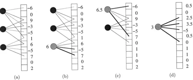
6-1 Instance of the set query problem . . . 6-2 Example run of the set query algorithm

Chapter 1

Introduction

In recent years, a new "linear" approach for obtaining a succinct approximate repre-sentation of n-dimensional vectors (or signals) has been discovered. For any signal x, the representation is equal to Ax, where A is an m x n matrix, or possibly a random variable chosen from some distribution over such matrices. The vector Ax is often referred to as the measurement vector or linear sketch of x. Although m is typically much smaller than n, the sketch Ax often contains plenty of useful information about the signal x.

A particularly useful and well-studied problem is that of stable sparse recovery. The problem is typically defined as follows: for some norm parameters p and q and an approximation factor C > 0, given Ax, recover a vector x' such that

|x' -

xII

< C - Errk(x), where Errk(x) = _{k-sparse x}min ||i - x|j| (1.1)

where we say that 5 is k-sparse if it has at most k non-zero coordinates. Sparse recovery has applications to numerous areas such as data stream computing [40,

29] and compressed sensing [6, 17], notably for constructing imaging systems that acquire images directly in compressed form (e.g., [18, 41]). The problem has been a subject of extensive study over the last several years, with the goal of designing schemes that enjoy good "compression rate" (i.e., low values of m) as well as good algorithmic properties (i.e., low encoding and recovery times). It is known that there

exist distributions of matrices A and associated recovery algorithms that for any x with high probability produce approximations x' satisfying Equation (1.1) with fp = fq = f₁, constant approximation factor C = 1 + e, and sketch length m =

0(k log(n/k))1_{. Similar results for other combinations of fp/f norms are known as}

well. In comparison, using a non-linear approach, one could obtain a shorter sketch of length 0(k): it suffices to store the k coefficients with the largest absolute values, together with their indices.

This thesis has two main parts. The first part is a tight lower bound on the number of measurements for general sparse recovery, and the second part introduces a useful primitive for circumventing the lower bound in special cases of sparse recovery.

1.1

A lower bound

Surprisingly, it was not known if the 0(k log(n/k)) bound on measurements for linear sketching could be improved upon2_{, and 0(k) sketch length was known to suffice if} the signal vectors x are required to be exactly k-sparse [1]. This raised hope that the 0(k) bound might be achievable even for general vectors x. Such a scheme would have been of major practical interest, since the sketch length determines the compression ratio, and for large n any extra log n factor worsens that ratio tenfold.

In the first part of this thesis we show that, unfortunately, such an improvement is not possible. We address two types of recovery scheme:

" A deterministic one, which involves a fixed matrix A and a recovery algorithm

which work for all signals x. The aforementioned results of [6] and others are examples of such schemes.

* A randomized one, where the matrix A is chosen at random from some distri-bution, and for each signal x the recovery procedure is correct with constant

'In particular, a random Gaussian matrix [10] or a random sparse binary matrix ([28], building on [9, 13]) has this property with overwhelming probability. See [27] for an overview.

2_{The lower bound of Q(k}

log(n/k)) was known to hold for specific recovery algorithms, specific

probability. Some of the early schemes proposed in the data stream literature (e.g., [9, 13]) belong to this category.

Our main result in this section is that, even in the randomized case, the sketch length m must be at least Q(k log(n/k)). By the aforementioned result of [6] this bound is tight. Thus, our results show that the linear compression is inherently more costly than the simple non-linear approach. Chapters 3 and 4 contain this result.

1.2

Set query algorithm

Because it has proved impossible to improve on the sketch size in the general sparse recovery problem, recently there has been a body of work on more restricted problems that are amenable to more efficient solutions. This includes model-based compressive

sensing

[4],

which imposing additional constraints (or models) on x beyond near-sparsity. Examples of models include block sparsity, where the large coefficients tend to cluster together in blocks [4, 21]; tree sparsity, where the large coefficients form a rooted, connected tree structure [4, 37]; and being Zipfian, where we require that the histogram of coefficient size follow a Zipfian (or power law) distribution.

A sparse recovery algorithm needs to perform two tasks: locating the large

coef-ficients of x and estimating their value. Existing algorithms perform both tasks at the same time. In contrast, we propose decoupling these tasks. In models of interest, including Zipfian signals and block-sparse signals, existing techniques can locate the large coefficients more efficiently or accurately than they can estimate them. Prior to this work, however, estimating the large coefficients after finding them had no better solution than the general sparse recovery problem. We fill this gap by giving an optimal method for estimating the values of the large coefficients after locating them. We refer to this task as the Set Query Problema.

Main result. (Set Query Algorithm.) We give a randomized distribution over

0(k) x n binary matrices A such that, for any vector x E R' and set S C {1,... , n}

3

The term "set query" is in contrast to "point query," used in e.g. [13] for estimation of a single coordinate.

with S| = k, we can recover an x' from Ax + v and S with

x' - _{XS||2 < C|X - XS||2 + 11v12)}

where xs _{E R"n equals x over S and zero elsewhere. The matrix A has 0(1) non-zero}

entries per column, recovery succeeds with probability 1 - k-( 1), and recovery takes O(k) time. This can be achieved for arbitrarily small e > 0, using O(k/e 2_{) rows. We}

achieve a similar result in the f1 norm.

The set query problem is useful in scenarios when, given the sketch of x, we have some alternative methods for discovering a "good" support of an approximation to x. This is the case, e.g., in block-sparse recovery, where (as we show in this paper) it is possible to identify "heavy" blocks using other methods. It is also a natural problem in itself. In particular, it generalizes the well-studied point query

problem [13], which considers the case that S is a singleton. We note that although

the set query problem for sets of size k can be reduced to k instances of the point query problem, this reduction is less space-efficient than the algorithm we propose, as elaborated in Chapters 5 and 6.

Chapter 2

Overview of Lower Bound

This chapter gives intuition and related work for our lower bounds. Proofs and further detail lie in Chapters 3 and 4.

2.1

Our techniques

On a high level, our approach is simple and natural, and utilizes the packing approach: we show that any two "sufficiently" different vectors x and x' are mapped to images

Ax and Ax' that are "sufficiently" different themselves, which requires that the image

space is "sufficiently" high-dimensional. However, the actual arguments are somewhat subtle.

Consider first the (simpler) deterministic case. We focus on signals x = y + z, where y can be thought of as the "head" of the signal and z as the "tail". The "head" vectors y come from a set Y that is a binary error-correcting code, with a minimum distance Q(k), where each codeword has weight k. On the other hand, the "tail" vectors z come from an f1 ball (say B) with a radius that is a small fraction of k. It can be seen that for any two elements y, y' E Y, the balls y + B and y'+ B, as well as their images, must be disjoint. At the same time, since all vectors x live in a "large" E1 ball B' of radius 0(k), all images Ax must live in a set AB'. The key observation is that the set AB' is a scaled version of A(y + B) and therefore the ratios of their volumes can be bounded by the scaling factor to the power of the dimension m. Since

the number of elements of Y is large, this gives a lower bound on m.

Unfortunately, the aforementioned approach does not seem to extend to the ran-domized case. A natural approach would be to use Yao's principle, and focus on showing a lower bound for a scenario where the matrix A is fixed while the vectors

x = y + z are "random". However, this approach fails, in a very strong sense.

Specif-ically, we are able to show that there is a distribution over matrices A with only 0(k) rows so that for a fixed y E Y and z chosen uniformly at random from the small ball

B, we can recover y from A(y + z) with high probability. In a nutshell, the reason is

that a random vector from B has an £2 norm that is much smaller than the f2 norm

of elements of Y (even though the f1 norms are comparable). This means that the vector x is "almost" k-sparse (in the £2 norm), which enables us to achieve the 0(k)

measurement bound.

Instead, we resort to an altogether different approach, via communication

com-plexity [36). We start by considering a "discrete" scenario where both the matrix

A and the vectors x have entries restricted to the polynomial range

{--n

... nc} for some c = 0(1). In other words, we assume that the matrix and vector entries can be represented using 0(log n) bits. In this setting we show the following: there is a method for encoding a sequence of d = 0(klog(n/k) logn) bits into a vector x, so that any sparse recovery algorithm can recover that sequence given Ax. Since each entry of Ax conveys only 0(log n) bits, it follows that the number m of rows of A must be Q(klog(n/k)).

The encoding is performed by taking

log n

x = E jj

j=1

where D = 0(1) and the x are chosen from the error-correcting code Y defined as in the deterministic case. The intuition behind this approach is that a good f1/1 approx-imation to x reveals most of the bits of xlogn. This enables us to identify xlogn exactly using error correction. We could then compute Ax - Axiogn = A( E"- 1 Dizx), and

argument is that we would need the recovery algorithm to work for all xi, which would require lower probability of algorithm failure (roughly 1/ log n). To overcome this problem, we replace the encoding argument by a reduction from a related com-munication complexity problem called Augmented Indexing. This problem has been used in the data stream literature [11, 32] to prove lower bounds for linear algebra and norm estimation problems. Since the problem has communication complexity of Q(d), the conclusion follows.

We apply the argument to arbitrary matrices A by representing them as a sum A' + A", where A' has O(log n) bits of precision and A" has "small" entries. We then show that A'x = A(x + s) for some s with

||s|1,

< n--

||x1

1

₁. In the communication game, this means we can transmit A'x and recover Xlogn from A'(Eg " Dix,) =

A(Eg₁" D3-x + s). This means that the Augmented Indexing reduction applies to

arbitrary matrices as well.

2.2

Related Work

There have been a number of earlier works that have, directly or indirectly, shown lower bounds for various models of sparse recovery and certain classes of matrices and algorithms. Specifically, one of the most well-known recovery algorithms used in compressed sensing is fi-minimization, where a signal x E R' measured by matrix A is reconstructed as

x' := arg min||2||1.

2: Ai=Ax

Kashin and Temlyakov [34] gave a characterization of matrices A for which the above recovery algorithm yields the £2

/f

1 guarantee, i.e.,

l|x

- x'|₂

< Ck-1/

2

min

||x

-

2||1

k-sparse z

for some constant C, from which it can be shown that such an A must have m = Q(k log(n/k)) rows.

in-vestigated in this paper. Specifically, it is easy to observe that if the approximation

x' itself is required to be 0(k)-sparse, then the f2/f1 guarantee implies the f1/f1

guar-antee (with a somewhat higher approximation constant). For the sake of simplicity, in this paper we focus mostly on the E1

/E

1 guarantee. However, our lower bounds

apply to the E2/f1 guarantee as well: see footnote on page 31.

On the other hand, instead of assuming a specific recovery algorithm, Wain-wright [44] assumes a specific (randomized) measurement matrix. More specifically, the author assumes a k-sparse binary signal x E

{0,

a}", for some a > 0, to which is

added i.i.d. standard Gaussian noise in each component. The author then shows that with a random Gaussian matrix A, with each entry also drawn i.i.d. from the standard Gaussian, we cannot hope to recover x from Ax with any sub-constant probability of error unless A has m = _{Q(1 log 1) rows. The author also shows that for a =}

/k,

this is tight, i.e., that m = 8(k log(n/k)) is both necessary and sufficient. Although this is only a lower bound for a specific (random) matrix, it is a fairly powerful one and provides evidence that the often observed upper bound of O(k log(n/k)) is likely tight.

More recently, Dai and Milenkovic [15], extending on [24] and [26], showed an upper bound on superimposed codes that translates to a lower bound on the number of rows in a compressed sensing matrix that deals only with k-sparse signals but can tolerate measurement noise. Specifically, if we assume a k-sparse signal x E ([-t, t] n Z)", and that arbitrary noise y E Rn with

||p||1

< d is added to the measurement vector Ax, then if exact recovery is still possible, A must have had m > Ck log n/ log k rows, for some constant C = C(t, d) and sufficiently large n and k.1

Concurrently with our work, Foucart et al. [25] have done an analysis of Gelfand widths of fp-balls that implies a lower bound on sparse recovery. Their work essentially matches our deterministic lower bound, and does not extend to the randomized case.

1Here A is assumed to have its columns normalized to have Li-norm 1. This is natural since

otherwise we could simply scale A up to make the image points Ax arbitrarily far apart, effectively nullifying the noise.

2.3

Preliminaries

2.3.1

Notation

For n E Z+, we denote {1, ... , n} by [n]. Suppose x E R". Then for i C [n], xi E R denotes the value of the i-th coordinate in x. As an exception, ej E R" denotes the elementary unit vector with a one at position i. For S ; [n], xs denotes the vector x' E R" given by x' = xi if i E S, and x' = 0 otherwise. We use supp(x) to denote the support of x. We use upper case letters to denote sets, matrices, and random distributions. We use lower case letters for scalars and vectors.

We use Bpn(r) to denote the f, ball of radius r in R"; we skip the superscript n if it is clear from the context. For any vector x, we use

||l|0

to denote the "to norm of

x", i.e., the number of non-zero entries in x.

2.3.2

Sparse recovery

In this paper we focus on recovering sparse approximations x' that satisfy the following C-approximate f1/1 guarantee with sparsity parameter k:

|ix - '1|1 < C min ||x - .||. (2.1)

k-sparse

We define a C-approximate deterministic

4//1

recovery algorithm to be a pair (A, d) where A is an m x n observation matrix and !/ is an algorithm that, for any x, maps Ax (called the sketch of x) to some x' that satisfies Equation (2.1).

We define a C-approximate randomized

4//1

recovery algorithm to be a pair (A, d) where A is a random variable chosen from some distribution over m x n measurement matrices, and d is an algorithm which, for any x, maps a pair (A, Ax) to some x' that satisfies Equation (2.1) with probability at least 3/4.

Chapter 3

Deterministic Lower Bound

3.1

Proof

We will prove a lower bound on m for any C-approximate deterministic recovery algorithm. First we use a discrete volume bound (Lemma 1) to find a large set Y of points that are at least k apart from each other. Then we use another volume bound (Lemma 2) on the images of small f1 balls around each point in Y. If m is too small, some two images collide. But the recovery algorithm, applied to a point in the collision, must yield an answer close to two points in Y. This is impossible, so m must be large.

Lemma 1. (Gilbert-Varshamov) For any q, k E Z+,e E R+ with e < 1 - 1/q, there

exists a set Y

c {o,

1}qk of binary vectors with exactly k ones, such that Y has minimum Hamming distance 2ek and

log |Y| > (1 - Hq(e))k log q

where Hq is the q-ary entropy function Hq(x) = -x log, q - (1 - x) logq(1 - x).

See appendix for proof.

Lemma 2. Take an m x n real matrix A, positive reals e, p, A, and Y C Bp(A).

A(y + z) = A(+ -f).

Proof. If the statement is false, then the images of all

IY|

balls {y + B"n(eA)

I

y E Y}

are disjoint. However, those balls all lie within B"'((1 + c)A), by the bound on the norm of Y. A volume argument gives the result, as follows.

Let S = AB"n(1) be the image of the n-dimensional ball of radius 1 in m-dimensional space. This is a polytope with some volume V. The image of Bpn(eA) is a linearly scaled S with volume (eA) m_{V, and the volume of the image of B"((1 + e)A)}

is similar with volume ((1 + e)A)"mV. If the images of the former are all disjoint and

lie inside the latter, we have |Y (EA)"mV < ((1 + e)A)mV, or |Y| 5 (1 + 1/c)m. If Y

has more elements than this, the images of some two balls y + B(cA) and -Y+ B"(eA)

must intersect, implying the lemma. D

Theorem 3. Any C-approximate deterministic recovery algorithm must have

1 - H[/kj(1/2) _n

log(4 + 2C) k

Proof. Let Y be a maximal set of k-sparse n-dimensional binary vectors with

mini-mum Hamming distance k, and let -y = 1. By Lemma 1 with q = [n/kJ we have

log YI > (1 - HL/kj (1/2))k log [n/kJ.

Suppose that the theorem is not true; then m < log |Y| / log(4+2C) = log |Y| / log(1+

1/y), or

|YJ

> (1 + I)" Hence Lemma 2 gives us some y,V E Y and z,

C

Bi(yk) with A(y + z) = A(V +

Let w be the result of running the recovery algorithm on A(y+z). By the definition of a deterministic recovery algorithm, we have

ly + z - wl < C min ||y + z -Q k-sparse 9

- wlli - ||z|il C jzz||

and similarly || -

ll

< k, so

|1y - M1|1 ||y - w|1 + 11p - will = 2 Ck < k.

But this contradicts the definition of Y, so m must be large enough for the guarantee

to hold. L

Corollary 4. If C is a constant bounded away from zero, then m = Q(k log(n/k)). This suffices to lower bound the number of measurements for deterministic matri-ces. The next section gives evidence that this proof is hard to generalize to randomized matrices; hence in the next chapter we will take a different approach.

3.2

Randomized upper bound for uniform noise

The standard way to prove a randomized lower bound is to find a distribution of hard inputs, and to show that any deterministic algorithm is likely to fail on that distribution. In our context, we would like to define a "head" random variable y from a distribution Y and a "tail" random variable z from a distribution Z, such that any algorithm given the sketch of y + z must recover an incorrect y with non-negligible probability.

Using our deterministic bound as inspiration, we could take Y to be uniform over a set of k-sparse binary vectors of minimum Hamming distance k and Z to be uniform over the ball B1

(yk)

for some constant -y > 0. Unfortunately, as the

following theorem shows, one can actually perform a recovery of such vectors using only O(k) measurements; this is because lIz1|2 is very small (namely, O(k/in)) with

high probability.

Theorem 5. Let Y C R' be a set of signals with the property that for every distinct

yi, y2 E Y, ||y1 - y2112 > r, for some parameter r > 0. Consider "noisy signals"

x = y + z, where y

E

Y and z is a "noise vector" chosen uniformly at random from B1(s), for another parameter s > 0. Then using an m x n Gaussian measurement

matrix A = (1/vf)(g j), where gi 's are i.i.d. standard Gaussians, we can recover y E Y from A(y + z) with probability 1 - 1/n (where the probability is over both A

and z), as long as

0 rmn1/2 n1/2-1/m

( YJI/m lega/2 n

Because of this theorem, our geometric lower bound for deterministic matrices is hard to generalize to randomized ones. Hence in Chapter 4 we use a different technique to extend our results.

To prove the theorem we will need the following two lemmas.

Lemma 6. For any 6 > 0, Y1, Y2 E Y, Y1

#

Y2, and z E R , each of the following

holds with probability at least 1 - 6:

" ||A(y1 - Y2)112 > |1rn - y2112, and

"

||Az|2

(v(8/m)

log(1/6) +

1)11z12.

Proof. By standard arguments (see, e.g., [30]), for any D > 0 we have

Pr IIA(y1 - Y2)||2 1

y Y

2

112]

(

and

Pr[|Az||2 > D|z| 2] < e-m(D1)2/8

Setting both right-hand sides to 6 yields the lemma. l

Lemma 7. A random vector z chosen uniformly from B1(s) satisfies

Pr[||z112 > as log n/v/n] < 1/no-1.

Proof. Consider the distribution of a single coordinate of z, say, zi. The probability

density of IziI taking value t E [0, s] is proportional to the (n - 1)-dimensional volume of B "~0(s - t), which in turn is proportional to (s - t)- 1. Normalizing to ensure

the probability integrates to 1, we derive this probability as

p(Izi I = t) = k(s - t 24

It follows that, for any D E [0, s],

Pr[IziI

>

D]

=

(s

- t)" 1 _{dt = (1 - D/s)".}

In particular, for any a > 1,

Pr[Izi| > aslogn/n]= (1 - alogn/n)" < e

= 1/n".

Now, by symmetry this holds for every other coordinate zi of z as well, so by the union bound

Pr[lz||oo > as log n/n] < 1/no,

and since

||z||

₂ Vfi

||z||oo

for any vector z, the lemma follows. El

Proof of theorem. In words, Lemma 6 says that A cannot bring faraway signal points too close together, and cannot blow up a small noise vector too much. Now, we already assumed the signals to be far apart, and Lemma 7 tells us that the noise is indeed small (in E2 distance). The result is that in the image space, the noise is not enough to confuse different signals. Quantitatively, applying the second part of Lemma 6 with 3 = 1/n 2, and Lemma 7 with a = 3, gives us

[ log/2 n (slog3/2 s

n

||Az|2 <- 0 2 z|12 < O (mn)1/2 (3.1)

with probability > 1 - 2/n 2_{. On the other hand, given signal yi E Y, we know that}

every other signal Y2 E Y satisfies

||Y1

- Y2112 > r, so by the first part of Lemma 6

with J = _{1/(2n|Y|), together with a union bound over every Y2 E Y,}

|IA(y 1 - Y2)|12 >

3(

IY

)1

m 2 3(2nY)1/m (3.2)

holds for every Y2 E Y, Y2 -/ Y1, simultaneously with probability 1 - 1/(2n).

signal Y2 E Y, we are guaranteed that

IIA(y1

+ z) - Ay,1| 2 = ||Azj|2

< ||A(y1 - y2)||2 - ||Az||2 < |IA(y1 + z) - Ay21|2

for every Y2

#

Y1, so we can recover yi by simply returning the signal whose image is closest to our measurement point A(yi + z) in f2 distance. To achieve this, we can chain Equations (3.1) and (3.2) together (with a factor of 2), to see that

0 rm1/2n1/

2_-1/m

(y|1/m log3/2n

suffices. Our total probability of failure is at most 2/n 2 _{+ 1/(2n) < 1/n.}

The main consequence of this theorem is that for the setup we used in Chapter

3 to prove a deterministic lower bound of Q(k log(n/k)), if we simply draw the noise

uniformly randomly from the same fi ball (in fact, even one with a much larger radius, namely, polynomial in n), this "hard distribution" can be defeated with just 0(k) measurements:

Corollary 8. If Y is a set of binary k-sparse vectors, as in Chapter 3, and noise z

is drawn uniformly at random from B1(s), then for any constant e > 0, m = 0(k/e) measurements suffice to recover any signal in Y with probability 1 - 1/n, as long as

0 k3/2+en1/2-c ( loga3/2 n

Proof. The parameters in this case are r = k and

IYI

<

(")

< (ne/k)k, so by Theorem

5, it suffices to have

<0 k3_/2_+k/mn1/2

-(k+l)/m

log3/2

Chapter 4

Randomized Lower Bound

In the previous chapter, we gave a simple geometric proof of the lower bound for deterministic matrices. We also showed that this proof does not easily generalize to randomized matrices. In this chapter, we use a different approach to show a lower bound for randomized as well as deterministic matrices. We will use a reduction from a communication game with a known lower bound on communication complexity.

The communication game will show that a message Ax must have a large number of bits. To show that this implies a lower bound on the number of rows of A, we will need A to be discrete. But if A is poorly conditioned, straightforward rounding could dramatically change its recovery characteristics. Therefore in Section 4.1 we show that it is sufficient to consider orthonormal matrices A. In Section 4.2 we define our communication game and show a lower bound on its communication complexity. In Section 4.3 we prove the lower bound.

4.1

Reducing to orthonormal matrices

Before we discretize by rounding, we need to ensure that the matrix is well condi-tioned. We show that without loss of generality, the rows of A are orthonormal.

We can multiply A on the left by any invertible matrix to get another measurement matrix with the same recovery characteristics. If we consider the singular value

diagonal, this means that we can eliminate U and make the entries of E be either 0 or 1. The result is a matrix consisting of m orthonormal rows. For such matrices, we prove the following:

Lemma 9. Consider any m x n matrix A with orthonormal rows. Let A' be the result

of rounding A to b bits per entry. Then for any v E R" there exists an s E R" with

A'v = A(v - s) and hsjjj < n22-b

iIV1.

Proof. Let A" = A - A' be the roundoff error when discretizing A to b bits, so each entry of A" is less than 2 -b. Then for any v and s = ATA"v, we have As = A"v and

js|\j = 11 AT A"vjj : \F||A~lv||l mV2-' ivii n22-b

lvJii.

4.2

Communication complexity

We use a few definitions and results from two-party communication complexity. For further background see the book by Kushilevitz and Nisan [36]. Consider the following communication game. There are two parties, Alice and Bob. Alice is given a string y E {0, 1}d. Bob is given an index i E [d], together with yi+1, yi+2, ... , yd. The

parties also share an arbitrarily long common random string r. Alice sends a single message M(y, r) to Bob, who must output yi with probability at least 3/4, where the probability is taken over r. We refer to this problem as Augmented Indexing. The communication cost of Augmented Indexing is the minimum, over all correct protocols, of the length of the message M(y, r) on the worst-case choice of r and y.

The next theorem is well-known and follows from Lemma 13 of [38] (see also

Lemma 2 of [31).

Proof. First, consider the private-coin version of the problem, in which both parties

can toss coins, but do not share a random string r (i.e., there is no public coin). Consider any correct protocol for this problem. We can assume the probability of error of the protocol is an arbitrarily small positive constant by increasing the length of Alice's message by a constant factor (e.g., by independent repetition and a majority vote). Applying Lemma 13 of [38] (with, in their notation, t = 1 and a = c' - d for a

sufficiently small constant c' > 0), the communication cost of such a protocol must be Q(d). Indeed, otherwise there would be a protocol in which Bob could output yi with probability greater than 1/2 without any interaction with Alice, contradicting that Pr[yi = 1/2] and that Bob has no information about yi. Our theorem now follows from Newman's theorem (see, e.g., Theorem 2.4 of

[35]),

which shows that the communication cost of the best public coin protocol is at least that of the private coin protocol minus O(log d) (which also holds for one-round protocols). L

4.3

Randomized lower bound theorem

Theorem 11. For any randomized f1/f1 recovery algorithm (A, &), with

approxima-tion factor C = 0(1), A must have m = Q(k log(n/k)) rows.

Proof. We shall assume, without loss of generality, that n and k are powers of 2, that

k divides n, and that the rows of A are orthonormal. The proof for the general case follows with minor modifications.

Let (A, d) be such a recovery algorithm. We will show how to solve the Augmented Indexing problem on instances of size d = Q(k log(n/k) log n) with communication cost 0(m log n). The theorem will then follow by Theorem 10.

Let X be the maximal set of k-sparse n-dimensional binary vectors with minimum Hamming distance k. From Lemma 1 we have log

IX|

= Q(k log(n/k)). Let d = [log

IX

IJ

log n, and define D = 2C + 3.

Alice is given a string y E {0, 1}d, and Bob is given i c [d] together with

Alice splits her string y into log n contiguous chunks y1_{, y}2_,

... , log" n, each

con-taining [log

XIJ

bits. She uses y3 as an index into X to choose xj. Alice defines

x = Dix1 + D2x2 + - - -+ Dlognxiogn.

Alice and Bob use the common randomness r to agree upon a random matrix A with orthonormal rows. Both Alice and Bob round A to form A' with b = [2(1 + log D) log n] = O(log n) bits per entry. Alice computes A'x and transmits it to Bob.

From Bob's input i, he can compute the value

j

= j(i) for which the bit y occurs in y'. Bob's input also contains yi+1,.. ,y7n, from which he can reconstruct

xj+1, ... , Xlog n, and in particular can compute

z = Dj+lxj+₁ + Dj+2x 3+2 +- + D "onXiog.

Bob then computes A'z, and using A'x and linearity, A'(x - z). Then

< kD _{i+log n}

||x - z||1 < kD' < k D 1 < kD20n

So from Lemma 9, there exists some s with A'(x - z) = A(x - z - s) and

|s|1

< n22-21ogn-21ogDiogn |x - zf11 < k.

Set w = x - z - _{s. Bob then runs the estimation algorithm d on A and Aw,}

obtaining w' with the property that with probability at least 3/4,

Now, min

11w

- w||1₁ <

||w

- Djx||, k-sparse t j-1

< ||s|| +

i

||D'xi||,

i=1 <k -D. D - 1 Hence Djxj - w'||K < ||Djxj - w|1K +

11w

- w'|| < (1 + C)||lDjxj - w

ll,

kDj 2

And since the minimum Hamming distance in X is k, this means

|lDix

- w'11₁ <

|Dix' -

w'11

for all x' E X, x' 7 x 1. So Bob can correctly identify xo with probability at least 3/4. From xo he can recover y3, and hence the bit yj that occurs in y'.

Hence, Bob solves Augmented Indexing with probability at least 3/4 given the message A'x. The entries in A' and x are polynomially bounded integers (up to scaling of A'), and so each entry of A'x takes O(logn) bits to describe. Hence, the communication cost of this protocol is O(m log n). By Theorem 10, m log n =

Q(k log(n/k) log n), or m = Q(k log(n/k)). 0

1_{Note that these bounds would still hold with minor modification if we replaced the E1 /E} guar-antee with the f2/L1 guarantee, so the same result holds in that case.

Chapter 5

Overview of Set Query Algorithm

The previous chapters show that the general sparse recovery problem cannot be solved with fewer than 8(k log(n/k)) linear measurements. However, many problems that can be cast as sparse recovery problems are special cases of the class; one can still hope to solve the special cases more efficiently. The rest of this thesis introduces the

set query problem, a useful primitive for this kind of problem. We show a particularly

efficient algorithm for this problem and two applications where our algorithm allows us to improve upon the best known results. Recall from the introduction that we

achieve the following:

We give a randomized distribution over 0(k) x n binary matrices A such that, for any vector x E R"n and set S C

{,.. . ,

n} with

|SI

= k, we can recover an x' from

Ax + v and S with

||x' - XS||2 < C(|Ix - XS12 + |1v112)

where xs E R' equals x over S and zero elsewhere. The matrix A has 0(1) non-zero entries per column, recovery succeeds with probability 1 - k-9(), and recovery takes 0(k) time. This can be achieved for arbitrarily small e > 0, using 0(k/e2) rows. We achieve a similar result in the 4 norm.

5.1

Our techniques

Our method is related to existing sparse recovery algorithms, including Count-Sketch [9] and Count-Min [13]. In fact, our sketch matrix A is almost identical to the one used in Count-Sketch-each column of A has d random locations out of 0(kd) each inde-pendently set to ±1, and the columns are indeinde-pendently generated. We can view such a matrix as "hashing" each coordinate to d "buckets" out of 0(kd). The difference is that the previous algorithms require 0(k log k) measurements to achieve our error bound (and d = 0(log k)), while we only need 0(k) measurements and d = 0(1).

We overcome two obstacles to bring d down to 0(1) and still achieve the error bound with high probability1. First, in order to estimate the coordinates xi, we need a more elaborate method than, say, taking the median of the buckets that i was hashed into. This is because, with constant probability, all such buckets might contain some other elements from S (be "heavy") and therefore using any of them as an estimator for y2 would result in too much error. Since, for super-constant values of

|S|,

it is

highly likely that such an event will occur for at least one i E S, it follows that this

type of estimation results in large error.

We solve this issue by using our knowledge of S. We know when a bucket is "corrupted" (that is, contains more than one element of S), so we only estimate coordinates that lie in a large number of uncorrupted buckets. Once we estimate a coordinate, we subtract our estimation of its value from the buckets it is contained in. This potentially decreases the number of corrupted buckets, allowing us to estimate more coordinates. We show that, with high probability, this procedure can continue until it estimates every coordinate in S.

The other issue with the previous algorithms is that their analysis of their prob-ability of success does not depend on k. This means that, even if the "head" did not interfere, their chance of success would be a constant (like 1 - ₂-(d)) rather than high probability in k (meaning 1 - k~(d)). We show that the errors in our estimates of coordinates have low covariance, which allows us to apply Chebyshev's inequality

to get that the total error is concentrated around the mean with high probability.

5.2

Related work

A similar recovery algorithm (with d = 2) has been analyzed and applied in a

stream-ing context in [23]. However, in that paper the authors only consider the case where the vector y is k-sparse. In that case, the termination property alone suffices, since there is no error to bound. Furthermore, because d = 2 they only achieve a constant probability of success. In this paper we consider general vectors y so we need to make sure the error remains bounded, and we achieve a high probability of success.

5.3

Applications

Our efficient solution to the set query problem can be combined with existing tech-niques to achieve sparse recovery under several models.

We say that a vector x follows a Zipfian or power law distribution with parameter a if [Xr(i) = E(8Xr(l)

|i~)

where r(i) is the location of the ith largest coefficient in x.

When a > 1/2, x is well approximated in the f2 norm by its sparse approximation.

Because a wide variety of real world signals follow power law distributions

([39,

5]),

this notion (related to "compressibility" 2) is often considered to be much of the reason why sparse recovery is interesting

([4,

7]). Prior to this work, sparse recovery of power law distributions has only been solved via general sparse recovery methods:

(1

+ e) Err2(x) error in 0(k log(n/k)) measurements.

However, locating the large coefficients in a power law distribution has long been easier than in a general distribution. Using 0(k log n) measurements, the Count-Sketch algorithm [9] can produce a candidate set S C {1 .. ... , b} with |SI= 0(k) that includes all of the top k positions in a power law distribution with high probability (if a > 1/2). We can then apply our set query algorithm to recover an approximation

x' to xS. _{Because we already are using 0(k log n) measurements on Count-Sketch,} 2_{A signal is "compressible" when}

_|xr(i)l

_{= O(Ixr(1)I}

j) rather than E(Ixr(1) I -a) [4]. This allows it to decay very quickly then stop decaying for a while; we require that the decay be continuous.

we use O(k log n) rather than O(k) measurements in the set query algorithm to get an 6//log n rather than e approximation. This lets us recover an x' with O(k log n)

measurements with

|1X' -X1|2 < 1 + C Err 2(X). log n)

This is especially interesting in the common regime where k < nl-C for some constant

c > 0. Then no previous algorithms achieve better than a (1+ c) approximation with

O(k log n) measurements, and the lower bound in [16] shows that any 0(1) approxi-mation requires Q(k log n) measurements3_{. This means at E(k log n) measurements,}

the best approximation changes from w(1) to 1 + o(1).

Another application is that of finding block-sparse approximations. In this case, the coordinate set

{1...

n} is partitioned into n/b blocks, each of length b. We define

a (k, b)-block-sparse vector to be a vector where all non-zero elements are contained in at most k/b blocks. An example of block-sparse data is time series data from n/b locations over b time steps, where only k/b locations are "active". We can define

Err(k,b)(x) = min _-11X - 112 (k,b)-block-sparse x

The block-sparse recovery problem can be now formulated analogously to Equa-tion 1.1. Since the formulaEqua-tion imposes restricEqua-tions on the sparsity patterns, it is natural to expect that one can perform sparse recovery from fewer than O(k log(n/k)) measurements needed in the general case. Because of that reason and its practical relevance, the problem of stable recovery of variants of block-sparse approximations has been recently a subject of extensive research (e.g., see [22, 42, 4, 8]). The state of the art algorithm has been given in [4], who gave a probabilistic construction of a single m x n matrix A, with m = 0(k + log n), and an n log0 1) n-time algorithm for performing the block-sparse recovery in the f1 norm (as well as other variants). If the blocks have size Q(log n), the algorithm uses only 0(k) measurements, which is a substantial improvement over the general bound. However, the approximation factor 3_{The lower bound only applies to geometric distributions, not Zipfian ones. However, our}

al-gorithm applies to more general sub-Zipfian distributions (defined in Section 7.1), which includes both.

C guaranteed by that algorithm was super-constant.

In this paper, we provide a distribution over matrices A, with m = O(k + ! log n), which enables solving this problem with a constant approximation factor and in the

f2 norm, with high probability. As with Zipfian distributions, first one algorithm tells

us where to find the heavy hitters and then the set query algorithm estimates their values. In this case, we modify the algorithm of [2] to find block heavy hitters, which enables us to find the support of the k _bb "most significant blocks" using O( log n)

measurements. The essence is to perform dimensionality reduction of each block from b to O(log n) dimensions, then estimate the result with a linear hash table. For each block, most of the projections are estimated pretty well, so the median is a good estimator of the block's norm. Once the support is identified, we can recover the coefficients using the set query algorithm.

5.4

Preliminaries

5.4.1

Notation

For n

E

Z+, we denote {... , n} by [n]. Suppose x E R". Then for i E [n], xi E R

denotes the value of the i-th coordinate in x. As an exception, e E R"n denotes the elementary unit vector with a one at position i. For S C [n], xs denotes the vector z' E R' given by x' = xi if i E S, and x' = 0 otherwise. We use supp(x) to denote the support of x. We use upper case letters to denote sets, matrices, and random distributions. We use lower case letters for scalars and vectors.

5.4.2

Negative association

This paper would like to make a claim of the form "We have k observations each of whose error has small expectation and variance. Therefore the average error is small with high probability in k." If the errors were independent this would be immediate from Chebyshev's inequality, but our errors depend on each other. Fortunately, our errors have some tendency to behave even better than if they were independent:

the more noise that appears in one coordinate, the less remains to land in other coordinates. We use negative dependence to refer to this general class of behavior. The specific forms of negative dependence we use are negative association and approzimate

Chapter 6

Set-Query Algorithm

Theorem 12. We give a randomized sparse binary sketch matrix A and recovery

algorithm d, such that for any x E R", S C [n] with

SI

= k, x' = d(Ax+v, S) E R"

has supp(x') C S and

||x - XS|2 E(||x - XS||2 + ||v|2)

with probability at least 1 per column, and c runs

We can achieve

l|x'

-with only O(fk) rows.

- 1/kc. Our A has O( pk) rows and 0(c) non-zero entries

in O(ck) time.

xs||1 < c(|lx - xs||1 +

||v|1)

under the same conditions, but

We will first show Theorem 12 for a constant c = 1/3 rather than for general c. Parallel repetition gives the theorem for general c, as described in Subsection 6.7. We will also only show it with entries of A being in {0, 1, -1}. By splitting each

row in two, one for the positive and one for the negative entries, we get a binary matrix with the same properties. The paper focuses on the more difficult f2 result;

6.1

Intuition

We call xs the "head" and x - xS _{the "tail." The head probably contains the heavy}

hitters, with much more mass than the tail of the distribution. We would like to estimate xs with zero error from the head and small error from the tail with high probability.

Our algorithm is related to the standard Count-Sketch [9] and Count-Min [13] algorithms. In order to point out the differences, let us examine how they perform on this task. These algorithms show that hashing into a single w = 0(k) sized hash table is good in the sense that each point xi has:

1. Zero error from the head with constant probability (namely 1 -W).

2. A small amount of error from the tail in expectation (and hence with constant probability).

They then iterate this procedure d times and take the median, so that each estimate has small error with probability 1 - ₂-2(d). With d = O(log k), we get that all k estimates in S are good with 0(k log k) measurements with high probability in k. With fewer measurements, however, some xi will probably have error from the head.

If the head is much larger than the tail (such as when the tail is zero), this is a major

problem. Furthermore, with 0(k) measurements the error from the tail would be small only in expectation, not with high probability.

We make three observations that allow us to use only 0(k) measurements to estimate xs with error relative to the tail with high probability in k.

1. The total error from the tail over a support of size k is concentrated more

strongly than the error at a single point: the error probability drops as k-(d)

rather than 2-(d).

2. The error from the head can be avoided if one knows where the head is, by modifying the recovery algorithm.

3. The error from the tail remains concentrated after modifying the recovery

For simplicity this paper does not directly show (1), only (2) and (3). The mod-ification to the algorithm to achieve (2) is quite natural, and described in detail in Section 6.2. Rather than estimate every coordinate in S immediately, we only esti-mate those coordinates which mostly do not overlap with other coordinates in S. In particular, we only estimate xi as the median of at least d - 2 positions that are not in the image of S

\

{i}.

Once we learn xi, we can subtract Axiej from the observed

Ax and repeat on A(x - xiej) and S \ {i}. Because we only look at positions that

are in the image of only one remaining element of S, this avoids any error from the head. We show in Section 6.3 that this algorithm never gets stuck; we can always find some position that mostly doesn't overlap with the image of the rest of the remaining support.

We then show that the error from the tail has low expectation, and that it is strongly concentrated. We think of the tail as noise located in each "cell" (coordinate in the image space). We decompose the error of our result into two parts: the "point error" and the "propagation". The point error is error introduced in our estimate of some xi based on noise in the cells that we estimate xi from, and equals the median of the noise in those cells. The "propagation" is the error that comes from point error in estimating other coordinates in the same connected component; these errors propagate through the component as we subtract off incorrect estimates of each xi.

Section 6.4 shows how to decompose the total error in terms of point errors and the component sizes. The two following sections bound the expectation and variance of these two quantities and show that they obey some notions of negative dependence1. We combine these errors in Section 6.7 to get Theorem 12 with a specific c (namely

c = 1/3). We then use parallel repetition to achieve Theorem 12 for arbitrary c.

6.2

Algorithm

We describe the sketch matrix A and recovery procedure in Algorithm 6.2.1. Un-like Count-Sketch [9] or Count-Min [13], our A is not split into d hash tables of size

O(k). Instead, it has a single w = O(d 2_k/e2_{) sized hash table where each}

coordi-nate is hashed into d unique positions. We can think of A as a random d-uniform hypergraph, where the non-zero entries in each column correspond to the terminals of a hyperedge. We say that A is drawn from Gd(w, n) with random signs associated with each (hyperedge, terminal) pair. We do this so we will be able to apply existing theorems on random hypergraphs.

Figure 6-1 shows an example Ax for a given x, and Figure 6-2 demonstrates running the recovery procedure on this instance.

Definition of sketch matrix A. For a constant d, let A be a w x n - 0( k) x n

matrix where each column is chosen independently uniformly at random over all exactly d-sparse columns with entries in

{-1,

0, 1}. We can think of A as the incidence

matrix of a random d-uniform hypergraph with random signs.

Recovery procedure.

1: procedure SETQUERY(A, S, b) r> Recover approximation x' to xs from

b = Ax + v

2: T <- S

3: while |TI > 0 do

4: Define P(q) =

{j

I

Aqj 5 0,

j

E T} as the set of hyperedges in T that contain q.

5: Define L = {q | Aqj

#

_{0, P(q)j = 1} as the set of isolated vertices in} hyperedge

j.

6: Choose a random

j

E T such that |Lj > d - 1. If this is not possible, find

a random

j

E T such that

ILI

> d - 2. If neither is possible, abort. 7: _{x +-- medianqEL Aqjbq} 8: b <- b - x'Aej 9: T - T\{j} 10: end while 11: return x' 12: end procedure