Remote Sensing and Cropping Practices: A Review

HAL Id: halshs-02438951

https://halshs.archives-ouvertes.fr/halshs-02438951

Submitted on 25 May 2021

HAL is a multi-disciplinary open access

archive for the deposit and dissemination of

sci-entific research documents, whether they are

pub-lished or not. The documents may come from

teaching and research institutions in France or

abroad, or from public or private research centers.

L’archive ouverte pluridisciplinaire HAL, est

destinée au dépôt et à la diffusion de documents

scientifiques de niveau recherche, publiés ou non,

émanant des établissements d’enseignement et de

recherche français ou étrangers, des laboratoires

publics ou privés.

Distributed under a Creative Commons Attribution| 4.0 International License

Agnes Begue, Damien Arvor, Beatriz Bellon, Julie Betbeder, Diego de

Abelleyra, Rodrigo P. D. Ferraz, Valentine Lebourgeois, Camille Lelong,

Margareth Simoes, Santiago R. Verón

To cite this version:

Agnes Begue, Damien Arvor, Beatriz Bellon, Julie Betbeder, Diego de Abelleyra, et al..

Re-mote Sensing and Cropping Practices: A Review. ReRe-mote Sensing, MDPI, 2018, 10 (2), pp.99.

�10.3390/rs10010099�. �halshs-02438951�

Review

Remote Sensing and Cropping Practices: A Review

Diego de Abelleyra5, Rodrigo P. D. Ferraz6, Valentine Lebourgeois1,2, Camille Lelong1,2, Margareth Simões6,7and Santiago R. Verón5,8

1 _{CIRAD, UMR TETIS, Maison de la Télédétection, 500 rue J.-F. Breton, 34093 Montpellier, France;}

beatriz.bellon@cirad.fr (B.B.); Valentine.Lebourgeois@cirad.fr (V.L.); camille.lelong@cirad.fr (C.L.)

2 _{CIRAD, Univ. Montpellier, 34 Montpellier, France; julie.betbeder@cirad.fr}

3 _{CNRS, UMR 6554 LETG-Univ. Rennes 2, 35043 Rennes, France; damien.arvor@univ-rennes2.fr} 4 _{CIRAD, UPR Forests & Societies, 34398 Montpellier, France}

5 _{INTA, Instituto de Clima y Agua, Hurlingham Buenos Aires 1686, Argentina;}

deabelleyra.diego@inta.gob.ar (D.d.A.); veron.santiago@inta.gob.ar (S.R.V.)

6 _{EMBRAPA Embrapa Solos, Rio de Janeiro 22460-000, Brazil; rodrigo.demonte@embrapa.br (R.P.D.F.);}

margareth.simoes@embrapa.br (M.S.)

7 _{Rio de Janeiro State University (UERJ/FEN/DESC/PPGMA), Rio de Janeiro 20550-900, Brazil} 8 _{Facultad de Agronomia—Universidad de Buenos Aires and CONICET, Buenos Aires 1417, Argentina}

* Correspondence: agnes.begue@cirad.fr; Tel.: +33-4-67-54-87-54

Received: 29 September 2017; Accepted: 9 January 2018; Published: 12 January 2018

Abstract:For agronomic, environmental, and economic reasons, the need for spatialized information about agricultural practices is expected to rapidly increase. In this context, we reviewed the literature on remote sensing for mapping cropping practices. The reviewed studies were grouped into three categories of practices: crop succession (crop rotation and fallowing), cropping pattern (single tree crop planting pattern, sequential cropping, and intercropping/agroforestry), and cropping techniques (irrigation, soil tillage, harvest and post-harvest practices, crop varieties, and agro-ecological infrastructures). We observed that the majority of the studies were exploratory investigations, tested on a local scale with a high dependence on ground data, and used only one type of remote sensing sensor. Furthermore, to be correctly implemented, most of the methods relied heavily on local knowledge on the management practices, the environment, and the biological material. These limitations point to future research directions, such as the use of land stratification, multi-sensor data combination, and expert knowledge-driven methods. Finally, the new spatial technologies, and particularly the Sentinel constellation, are expected to improve the monitoring of cropping practices in the challenging context of food security and better management of agro-environmental issues.

Keywords: cropping system; crop succession; rotation; cropping pattern; multiple cropping; agroforestry; irrigation; soil tillage; harvest; intercropping; fallow

1. Introduction

In terms of productivity, use of natural resources, and farmer income, the importance of cropping practices has long been recognized by the international community, who thus defined the concept and guidelines of good agricultural practices (GAP) under the Food and Agriculture Organization (FAO) guidance [1]. The GAP aim at producing safe and healthy food and non-food agricultural products, while managing and enhancing environmental habitats. For this purpose, the guidelines encourage improved water and soil management, crop and fodder production, pest and disease control, and energy and waste management, at the farm scale.

As food is produced on a global scale, it is increasingly difficult for national governments and consumers to control the production process. Therefore, traceability and verification of good

agricultural practices is important [2] and to achieve this, the needs for spatial information are expected to grow rapidly.

Remote sensing has been proven to be an effective tool for monitoring cropping practices. Due to a large variety of on-board sensors on an increasing number of civilian satellites [3], the spectral and temporal properties of the land surface resulting from human practices can be captured and monitored at different spatial and temporal scales. However, a detailed literature analysis showed that less than 10% of the publications on remote sensing and agriculture actually focus on cropping practices [4].

Given its importance, a status report on the capabilities of remote sensing for mapping and characterizing cropping systems is overdue. Therefore, we reviewed the literature on remote sensing data and the methods used to produce spatial information on cropping practices. Notably, crop type mapping using remote sensing was not included, since it was already reviewed in recent publications [5,6]. The paper is structured as follows. First, we present a typology of the main cropping practices with their definitions, since agronomic-related vocabulary sometimes lacks precision in the remote sensing literature. We identified three main categories of practices: crop succession, cropping patterns, and cropping techniques. For each practice, we synthesize its agronomic, environmental, and socio-economic benefits, and review remote sensing-based studies used to detect and characterize these benefits. The most important features of each category are then highlighted and the research efforts needed to produce accurate and robust information on the cropping system are discussed. Finally, we recommend future research for the use of the new generation of Earth-observation systems for large scale applications.

2. Typology of the Cropping Practices

Some agronomic terms do not have an international and unique definition. Therefore, certain technical agronomic-related vocabulary is sometimes misused in remote sensing publications. To ensure clarity, we wanted to start this paper by defining the agronomic terms used hereafter, referring to the most common definitions, and respecting the agronomic conventions as closely as possible.

In this paper, “cropping practices” describes the elements of a cropping system. A cropping system refers to the crop type, sequence, and arrangement, and to the management techniques used on a particular field over a period of years [7,8]. The cropping system can be described by the following three components, each of them being defined by a set of cropping practices (Figure1): (1) a temporal component describing the sequence of crops or fallows for consecutive years, referred hereafter as “crop succession” (number 1 in Figure1); (2) a component describing the yearly sequence and spatial arrangement of crops and fallows in a particular land area, referred hereafter as “cropping pattern” (number 2 in Figure1); and (3) a crop management component that corresponds to the techniques, such as irrigation or soil tillage, implemented on a piece of land (number 3 in Figure1).

In the subsequent sections, only the cropping practices that were studied in remote sensing are presented, and highlighted in bold in Figure1. Some pastoral practices related to their production management are also included. Notably, the list of the studies reviewed in this paper is certainly incomplete as we were not aiming to be exhaustive but to report the representative results.

Figure 1. Typology and short definitions of the cropping system components, numbered 1 to 3, and

associated cropping practices, as used in this paper. Bold terms indicate the cropping practices that are reviewed in this paper.

3. Crop Succession

The term “crop succession” refers to the sequence of crops or fallows in consecutive years. Thus, monoculture, crop rotation, and fallowing, which is the practice of sequences of crop years and fallow years, are different types of crop succession. Differentiating between these three types of crop succession is important because they have different impacts on food production and natural resources management.

3.1. Monocropping and Crop Rotation

Crop rotation is a useful technique for soil management, controlling pathogens, pests, and weeds, for removing excess nutrients in the soil, and correcting nutrient deficiencies of soils. While monocropping is generally practiced in intensive agricultural farms, where large amounts of resources are available to improve the production process, crop rotation is a necessity for low-input farms. Crop rotation is a reasoned process where choosing the crop species for succession is not random, but follows recommended patterns [9]. For example, a nitrogen depleting crop should be followed by a nitrogen-fixing crop, and a low residue crop by a high biomass cover crop [10].

Monocropping and crop rotation can be directly assessed with annual crop type maps, by extracting the sequence of crop types at the field scale for more than two years. In the Midwestern United States, Stern et al. [11] analyzed 10 years of annual remote sensing crop classifications from the National Agricultural Statistics Service of the United States Department of Agriculture (USDA), to define the corn-soybean rotation dynamic in relation to the market prices. In the Kiev region, Ukraine, highly accurate crop type maps were produced using a combination of neural networks applied to optical and radar image time series acquired during the period of 2013 to 2015 [12,13]. A crop rotation violation map for the Bilotserkivskiy district was then produced, showing fields where winter wheat, winter rapeseed, sunflower, and maize were grown in the same fields for at least two or three years, contrary to the agricultural policy in place. Sahajpal et al. [14] developed the

Figure 1. Typology and short definitions of the cropping system components, numbered 1 to 3, and associated cropping practices, as used in this paper. Bold terms indicate the cropping practices that are reviewed in this paper.

3. Crop Succession

The term “crop succession” refers to the sequence of crops or fallows in consecutive years. Thus, monoculture, crop rotation, and fallowing, which is the practice of sequences of crop years and fallow years, are different types of crop succession. Differentiating between these three types of crop succession is important because they have different impacts on food production and natural resources management.

3.1. Monocropping and Crop Rotation

Crop rotation is a useful technique for soil management, controlling pathogens, pests, and weeds, for removing excess nutrients in the soil, and correcting nutrient deficiencies of soils. While monocropping is generally practiced in intensive agricultural farms, where large amounts of resources are available to improve the production process, crop rotation is a necessity for low-input farms. Crop rotation is a reasoned process where choosing the crop species for succession is not random, but follows recommended patterns [9]. For example, a nitrogen depleting crop should be followed by a nitrogen-fixing crop, and a low residue crop by a high biomass cover crop [10].

Monocropping and crop rotation can be directly assessed with annual crop type maps, by extracting the sequence of crop types at the field scale for more than two years. In the Midwestern United States, Stern et al. [11] analyzed 10 years of annual remote sensing crop classifications from the National Agricultural Statistics Service of the United States Department of Agriculture (USDA), to define the corn-soybean rotation dynamic in relation to the market prices. In the Kiev region, Ukraine, highly accurate crop type maps were produced using a combination of neural networks applied to optical and radar image time series acquired during the period of 2013 to 2015 [12,13]. A crop rotation violation map for the Bilotserkivskiy district was then produced, showing fields where winter

wheat, winter rapeseed, sunflower, and maize were grown in the same fields for at least two or three years, contrary to the agricultural policy in place. Sahajpal et al. [14] developed the Representative Crop Rotations Using Edit Distance (RECRUIT) algorithm that selects representative crop rotations by combining and analyzing maps of the major agricultural crops traded on the U.S. commodity markets, produced annually from remote sensing data by the USDA.

However, Mueller-Warran et al. [15] outlined that although converting multi-year land-use data into crop rotation history is relatively simple in theory, the presence of classification errors can severely compromise the results. Given this fact, they proposed using a matrix of logically forbidden or extremely unlikely year-to-year land use transitions to detect classification errors. Likewise, the use of a priori knowledge of the local rotation practices could be a research area for improving crop type identification by constraining classification models.

3.2. Crop-Fallow Rotation/Fallowing

Hereafter, fallow refers to arable land that is set aside for a period of time ranging from one to five or more years before being used again for cultivation. Fallow aims to regenerate natural resources, such as soil and water, after exploitation, and represents about 28% (4.4 million km2) of the global cropped areas [16]. Updated knowledge about the extent, frequency, and duration of fallow land provides baseline information for policy making and resource planning, such as cropland intensification vs. cropland area expansion [17] and allocation of scarce water resources for on-farm use [18].

Existing land use and land cover studies commonly merge the cropped and fallowed fields in a common class [19]. Due to the wide range of existing fallow practices, mapping of these areas is a difficult task [16]. A fallowed field may be confused with cropped fields due to climatic and soil conditions [20], cropping techniques [19], crop failure [16], or may be confused with surrounding ecosystems due to its natural regeneration.

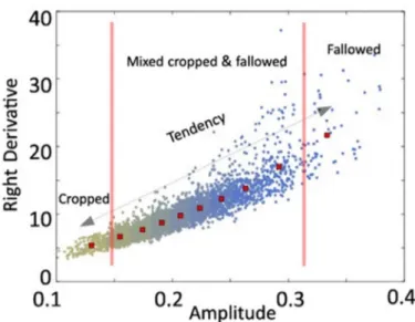
Despite these difficulties, examples of methods for fallow characterization using remote sensing data exist in the literature. This characterization is generally performed in three steps: (1) cropland mapping, (2) annual/seasonal fallow mapping inside the cropland mask using satellite time series, and (3) multi-annual analysis of the fallow maps to determine the fallowing frequency, also known as the fallow age. Xie et al. [21] showed that masking the non-agricultural areas blended with agricultural fields was a critical pre-processing step for distinguishing active crops and fallow lands. In Niger, Tong et al. [19] developed a classification approach based on the different phenological characteristics of the vegetation, including Normalized Difference Vegetation Index (NDVI), amplitude, and rate of decrease rate, as monitored by a MODerate-resolution Imaging Spectroradiometer (MODIS) 250 m resolution data. They showed that fallowed fields generally have a higher NDVI and a more rapid decrease than unmanured cropped fields (Figure2). In the Central Valley of California, Melton et al. [18] tracked land fallowing using a NDVI time series based on Landsat data completed with MODIS data, and monthly ground data collections. They used a decision-tree algorithm to evaluate the information about a set of phenological metrics extracted from the NDVI time series, and the land-use changes relative to previous years, to assign each field to a land-use class. The classification accuracy was above 85%, and the authors noticed that the primary sources of error were confusion between young fallows and recently planted perennial crop fields, and errors associated with field boundaries or partially planted fields. To overcome the constraints of ground data collection, for the same area, Wallace et al. [22] developed and applied a Fallow-land Algorithm based on Neighborhood and Temporal Anomalies (FANTA) that routinely mapped cropland status (cropped or fallowed) with user and producer accuracies over 75%. The FANTA algorithm compares the current greenness of a cultivated pixel to its historical greenness and to the greenness of all cultivated pixels within a defined spatial neighborhood. Good results were obtained applying FANTA to annual row crops, but the study encountered the same difficulty as Melton et al. [18] for perennial crops that have a much more diverse growth cycle.

Figure 2. Scatter plots illustrating the MODIS Normalized Difference Vegetation Index (NDVI) based phenological differences between unmanured cropped and fallowed land in Niger, from Tong et al. [19]. After the rainy season, a larger amplitude and a faster decrease were observed for the fallowed fields compared to the unmanured cropped fields.

The examples above show that fallows and the surrounding crops (especially perennial crops) or natural vegetation are commonly confused, and these confusions are spatially heterogeneous due to varying climatic and soil conditions, and cropping practices. As a result, methods to accurately monitor active, fallowed, and abandoned cropland are still lacking for many regions in the world [20]. Closely monitoring the vegetation development for the same piece of land over several years with regular satellite imagery acquisition and processing is one area to continue to explore.

4. Cropping Pattern

Cropping pattern is defined here as the yearly sequence and spatial arrangement of crops, or of crops and pasture, on a given piece of land. Multiple cropping is when more than one crop is involved, as opposed to single cropping.

4.1. Single Cropping

For single cropping, the cropping pattern refers to the spatial arrangement of the crops. The vast majority of the remote sensing studies address the spatial patterns of tree crops, such as orchards and vineyards. Few studies have reported on annual crop row orientation [23].

Tree Crop Planting Pattern

Tree crops represent a significant part of agricultural landscapes, and their specific cropping practices mean they must be mapped separately from annual crops. The knowledge of their presence and associated cropping practices contributes both to landscape ecology and economical surveys. Some tree crops, such as nut groves and vineyards, are eligible for support payments from the European Common Agricultural Policy for specific plot sizes and tree planting densities [24]. Remote sensing has thus been developed as a tool for subsidies control, for instance, with the first goal being to map the areas of permanent crops.

This subject appears to be a challenge for optical remote sensing because of the considerable spectral and spatial heterogeneity and variability in the object of study, such as for plant layout, density, and structure. As comprehensively described by Aksoy et al. [25], although some spectral features analysis succeeded in discriminating structured plots [26], automatic orchards and vineyards mapping methods have mostly been developed based on the textural approach, using various structural indicators such as indices derived from the co-occurrence matrix [27,28], autocorrelograms [29,30], Markov random fields [31], and frequential analysis [32–35]. Peña-Barragan et al. [36] showed

Figure 2.Scatter plots illustrating the MODIS Normalized Difference Vegetation Index (NDVI) based phenological differences between unmanured cropped and fallowed land in Niger, from Tong et al. [19]. After the rainy season, a larger amplitude and a faster decrease were observed for the fallowed fields compared to the unmanured cropped fields.

The examples above show that fallows and the surrounding crops (especially perennial crops) or natural vegetation are commonly confused, and these confusions are spatially heterogeneous due to varying climatic and soil conditions, and cropping practices. As a result, methods to accurately monitor active, fallowed, and abandoned cropland are still lacking for many regions in the world [20]. Closely monitoring the vegetation development for the same piece of land over several years with regular satellite imagery acquisition and processing is one area to continue to explore.

4. Cropping Pattern

Cropping pattern is defined here as the yearly sequence and spatial arrangement of crops, or of crops and pasture, on a given piece of land. Multiple cropping is when more than one crop is involved, as opposed to single cropping.

4.1. Single Cropping

For single cropping, the cropping pattern refers to the spatial arrangement of the crops. The vast majority of the remote sensing studies address the spatial patterns of tree crops, such as orchards and vineyards. Few studies have reported on annual crop row orientation [23].

Tree Crop Planting Pattern

Tree crops represent a significant part of agricultural landscapes, and their specific cropping practices mean they must be mapped separately from annual crops. The knowledge of their presence and associated cropping practices contributes both to landscape ecology and economical surveys. Some tree crops, such as nut groves and vineyards, are eligible for support payments from the European Common Agricultural Policy for specific plot sizes and tree planting densities [24]. Remote sensing has thus been developed as a tool for subsidies control, for instance, with the first goal being to map the areas of permanent crops.

This subject appears to be a challenge for optical remote sensing because of the considerable spectral and spatial heterogeneity and variability in the object of study, such as for plant layout, density, and structure. As comprehensively described by Aksoy et al. [25], although some spectral features analysis succeeded in discriminating structured plots [26], automatic orchards and vineyards mapping methods have mostly been developed based on the textural approach, using various structural

indicators such as indices derived from the co-occurrence matrix [27,28], autocorrelograms [29,30], Markov random fields [31], and frequential analysis [32–35]. Peña-Barragan et al. [36] showed that multispectral imagery is suitable to discriminate cover crops from olive trees and to estimate olive tree surface with good accuracy (92%). Panda et al. [37] reviewed several techniques used in fruit and nut crop management and described the methods used to differentiate orchards from other land uses, and how GIS and models can then be applied for analyses. No accurate discrimination of tree crop types has been achieved without a significant input of field knowledge.

Most remote sensing studies that addressed tree crop planting patterns focused on vineyards, and less on olive and nut groves. Even if some studies showed the feasibility of separating different cropping structures, such as simple row vs. pergola (continuous trelliswork) in large vineyards using decametric resolution images [38] with ASTER (Advanced Spaceborne Thermal Emission and Reflection Radiometer) data at a spatial resolution of 15 m, most authors highlighted the need for high spatial resolution images, with metric and sub-metric resolution, to detect intra-field cropping structure. The best imagery was acquired from Unmanned Aerial Vehicles (UAV) or UtraLight Aircrafts (ULA). Delenne et al. [39] showed that simple local Fourier analysis and co-occurrence matrix-based indices, applied to very high spatial resolution images acquired with an ULA, detected vineyards and characterized intra-field cropping patterns (simple row vs. pergola), and rows and inter-row orientation and scale. Along the same lines, Amoruso et al. [29] used a variogram-based texture algorithm to discriminate olive groves from forest and other vegetation land use classes. More generally, Yalniz and Aksoy [40] used wavelet analysis of image texture to discriminate between tree crops of various regularity, in terms of periodicity, orientation, and scale. Lefebvre et al. [41] also proposed wavelet decomposition for a textural pattern analysis, improving vineyard detection and cropping pattern (row orientation) characterization. However, some researchers consider Light Detection And Ranging (LiDAR) technologies as the more relevant tool to map tree crowns and derive structural information, and an abundance of three dimensional (3D) studies can be found in the literature for tree crop structure characterization based on LiDAR [42].

Several studies focused on tree crown status, using images at spatial resolutions smaller than one meter, after manual delineation of the tree [43]. Others developed methods and algorithms, such as local maximum filtering and valley-following, to automatically delineate tree crowns [44–46], where the tree detection ability is closely linked to the often sub-meter image spatial resolution. Most of these algorithms were developed to detect trees in forests, but obtain good results for fruit groves that display a simpler structure. Torres et al. [47] developed software (CLUstering Assessment or CLUAS) to provide some quantitative agronomical parameters and environmental indicators in olive groves, such as the number of olive trees, the size of each tree, the fraction of soil covered by trees, or the potential productivity based on density calculations. However, hyperspectral and/or UAV technologies are needed for good accuracy in tree detection [48]. Stereo imagery at very high spatial resolution, which obtains surface and elevation models, is also promising but only in situations with good contrast between the tree crown and its immediate environment to allow correct matching of the stereo pairs.

4.2. Multiple Cropping 4.2.1. Sequential Cropping

Sequential cropping consists of harvesting more than one crop sequentially during the same growing season. In areas with sufficient rainfall and a long frost-free period, one, two, or even three harvests are possible per year [49]. The main reason for adopting sequential cropping systems is economic since it creates a rapid increase in the land productivity. Nonetheless, sequential cropping can also be related to the adoption of ecological cropping practices. For example, the second crop is often sown both to benefit from the end of the rainy season and to enable the adoption of no-tillage practices [50,51]. By doing so, the soil quality is improved by limiting the loss of chemical products and

organic matter via erosion, and by retaining water for a longer period, which allow farmers to achieve better yields [50,51]. Sequential cropping may also help fight against crop diseases, as was the case with the Asiatic rust soybean disease, whose expansion in the Southern Amazon was aided by the soy monoculture. Finally, since double cropping increases crop production in existing agricultural areas, it limits land use changes such as tropical deforestation driven by agricultural expansion [52–54].

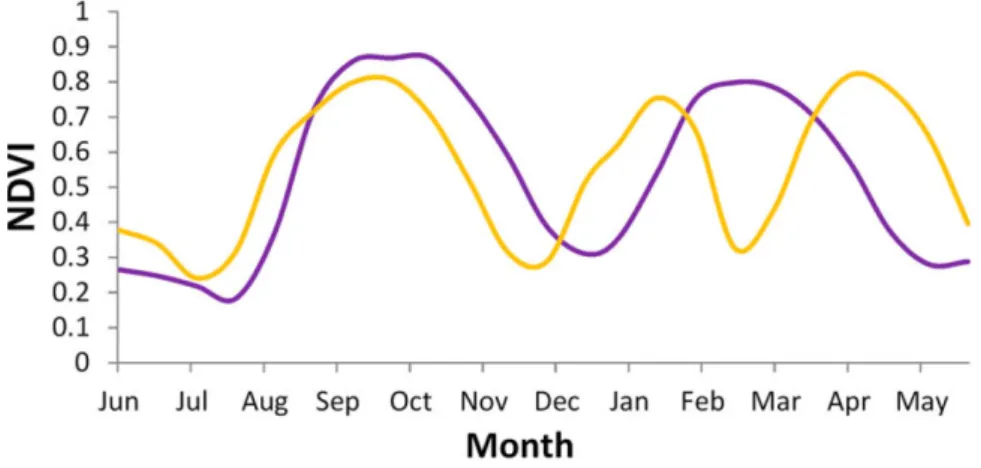
Remote sensing-based characterization of sequential multiple cropping relies on the use of high temporal resolution time series to ensure accurate monitoring of the phenological cycles [49,55] and capture the seasonal variability and crop calendars of sequential cropping systems (Figure3). Good expert knowledge of the local to regional agricultural practices is thus required. Coarse spatial-resolution satellite imagery with high revisiting frequencies, such as NOAA-AVHRR [56] (National Oceanic and Atmospheric Administration-Advanced Very High-Resolution Radiometer) or SPOT-VGT [57,58] (Satellite Pour l’Observation de la Terre-Vegetation) are usually preferred, but MODIS data has long received more attention for this type of application due to its daily acquisitions and 16-day composites of vegetation indices (Enhanced Vegetation Index (EVI) or NDVI) with a 250 m spatial resolution. MODIS data have been successfully used to map sequential multiple cropping in various agricultural areas with relatively large fields, especially in the United States, China, and Brazil. In the U.S. Great Plains (Kansas), Wardlow et al. [55] assessed the potential of NDVI and EVI time series to separate crop types and cropping systems, which were subsequently mapped [59]. In Northern and Central China, Mingwei et al. [49] and Qiu et al. [60] mapped single (cotton or maize) and double cropping systems (winter wheat-cotton, winter wheat-maize, and winter wheat-rice) based on Fourier and wavelet analysis, respectively. In the Brazilian Amazon, studies conducted at the local level explored the potential of MODIS vegetation index time series to discriminate single- and double-cropping systems (soybean and soybean-maize or soybean-cotton) [61,62]. These studies were then upscaled to regional-scale maps of these systems over the entire state of Mato Grosso [63–65].

Remote Sens. 2018, 10, 99 7 of 32

agricultural areas, it limits land use changes such as tropical deforestation driven by agricultural expansion [52–54].

Remote sensing-based characterization of sequential multiple cropping relies on the use of high temporal resolution time series to ensure accurate monitoring of the phenological cycles [49,55] and capture the seasonal variability and crop calendars of sequential cropping systems (Figure 3). Good expert knowledge of the local to regional agricultural practices is thus required. Coarse spatial-resolution satellite imagery with high revisiting frequencies, such as NOAA-AVHRR [56] (National Oceanic and Atmospheric Administration-Advanced Very High-Resolution Radiometer) or SPOT-VGT [57,58] (Satellite Pour l’Observation de la Terre-Vegetation) are usually preferred, but MODIS data has long received more attention for this type of application due to its daily acquisitions and 16-day composites of vegetation indices (Enhanced Vegetation Index (EVI) or NDVI) with a 250 m spatial resolution. MODIS data have been successfully used to map sequential multiple cropping in various agricultural areas with relatively large fields, especially in the United States, China, and Brazil. In the U.S. Great Plains (Kansas), Wardlow et al. [55] assessed the potential of NDVI and EVI time series to separate crop types and cropping systems, which were subsequently mapped [59]. In Northern and Central China, Mingwei et al. [49] and Qiu et al. [60] mapped single (cotton or maize) and double cropping systems (winter wheat-cotton, winter wheat-maize, and winter wheat-rice) based on Fourier and wavelet analysis, respectively. In the Brazilian Amazon, studies conducted at the local level explored the potential of MODIS vegetation index time series to discriminate single- and double-cropping systems (soybean and soybean-maize or soybean-cotton) [61,62]. These studies were then upscaled to regional-scale maps of these systems over the entire state of Mato Grosso [63– 65].

Figure 3. Example of the smoothed moderate-resolution imaging spectroradiometer (MODIS) Normalized Difference Vegetation Index (NDVI) time series profiles of sequential double-cropping and triple-cropping systems. These profiles show intensification practices adopted in South Asia that include growing two cycles of rice crop sequentially during the same growing season (purple line), and including a short growing cycle of grain legumes crops between the two rice cycles (orange line). Obtained from Gumma et al. [17].

In these studies, Vegetation Index (VI) time series are generally pre-processed to limit misclassification due to noisy data. Although the MODIS VI data are made of composite values, low noise VI values may remain in tropical areas with an intense rainy season. To correct these values, various smoothing algorithms can be used [66], as well as wavelet analysis [62]. Most of the studies then train supervised classifications with reference data, usually in the form of ground observations [49,63,64]. Unsupervised classification approaches are somewhat less common but have achieved good results when adopting hyperclustering methods [17,59,67]. Clustering approaches do not require ground data, which are time- and resource-consuming to collect, especially when data must be gathered twice during the growing season over large areas. However, labeling the final classes

Figure 3. Example of the smoothed moderate-resolution imaging spectroradiometer (MODIS) Normalized Difference Vegetation Index (NDVI) time series profiles of sequential double-cropping and triple-cropping systems. These profiles show intensification practices adopted in South Asia that include growing two cycles of rice crop sequentially during the same growing season (purple line), and including a short growing cycle of grain legumes crops between the two rice cycles (orange line). Obtained from Gumma et al. [17].

In these studies, Vegetation Index (VI) time series are generally pre-processed to limit misclassification due to noisy data. Although the MODIS VI data are made of composite values, low noise VI values may remain in tropical areas with an intense rainy season. To correct these values, various smoothing algorithms can be used [66], as well as wavelet analysis [62]. Most of the studies then train supervised classifications with reference data, usually in the form of ground observations [49,63,64]. Unsupervised classification approaches are somewhat less common but have

achieved good results when adopting hyperclustering methods [17,59,67]. Clustering approaches do not require ground data, which are time- and resource-consuming to collect, especially when data must be gathered twice during the growing season over large areas. However, labeling the final classes relies on adequate knowledge of the local to regional agricultural practices, which allows relating the different phenological cycles to the crop calendars to ultimately identify crop types.

The main issue for classification is the high intra-class variability in the sequential cropping systems. The same cropping system can be characterized by different crop calendars due to regional climatic differences [52], specific climatic events in some given years (e.g., a longer dry season that caused delayed sowing), and logistical issues, such as the sowing period lasting a few months in very large farms. To address this issue, different approaches are implemented to classify the satellite time series. Time series may be processed to extract features, such as in Morton et al. [68] where 36 metrics from MODIS VI time series were computed, including NDVI and EVI minimum, maximum, mean, median, amplitude, and standard deviation for annual wet and dry seasons, which were subsequently classified. Arvor et al. [63] searched for the best dates of the time series that maximized the separability distance between the EVI profiles of six classes of cropping systems. Innovative techniques, such as Fourier analysis [49] or wavelet analysis [60], provide a new representation of image time series, allowing for a finer analysis of vegetation phenology. Nonetheless, these techniques are based on a reduction dimension which implies a loss of information. To address this issue, new techniques, such as Dynamic Time Warping approaches with temporal weights, were successfully tested to classify land cover classes including single and double cropping systems, based on shape matching of MODIS EVI time series [69]. Bailly et al. [70] implemented a Dense Bag-of-Temporal-SIFT-Words approach, which involves representing vegetation index time series in sequences of local features, such as peaks and constant growth. These features were then used to build histograms of patterns corresponding to new time series representations to be classified by traditional classifiers, such as support vector machine (SVM).

Complementary studies evaluated the potential of Synthetic Aperture Radar (SAR) imagery for monitoring multiple cropping systems. For example, some studies demonstrated the potential of ENVISAT ASAR (Advanced Synthetic Aperture Radar) time series to detect single-, double-, and triple-cropped rice areas in the Mekong Delta River [71,72]. Bouvet et al. [71] showed that the detection of a high backscatter increase at the beginning of the growing cycle allowed for the production of rice maps early in the season. However, these studies were limited by the poor acquisition frequency of the available SAR data. They used incidence angle normalization methods and/or temporal averaging to combine acquisitions from multiple tracks and years. This limitation is now outdated due to the launched SAR Sentinel-1 sensor that provides dense time series with a temporally-consistent incidence angle.

4.2.2. Intercropping/Agroforestry

Few remote sensing studies address intercropping. This can be explained by the infra-metric scale of the intra-field variability of mixed crop fields. Only agroforestry systems can be considered as an exception, and are detailed hereafter.

Agroforestry is the practice of growing crops and trees, and sometimes keeping animals, together. This is a multifunctional land-use system and technology that provides a wide range of economic, sociocultural, and environmental benefits [73,74]. The ecologically-based dynamic integration of trees on farms and in the agricultural landscape diversifies and sustains production for land users at all levels, enhancing food supply, income, health, and environmental sustainability, even in the most industrialized nations [75]. Among these benefits, agroforestry supports food production by enhancing fertility [76,77], controlling soil erosion [78,79], improving water quality [80,81]), and by sequestering substantial quantities of carbon [82,83].

Agroforestry is a challenging cropping system to monitor using remote sensing because of its spatial heterogeneity and complexity. Agroforestry cropping patterns can range from the regular

intercropping of two or more types of crops, whose rows vary from one to five meters in width, to a totally random distribution of dozens of different tree species and sizes in a closed canopy. Due to this wide range of heterogeneity, discriminating different agroforestry systems based only on their spectral signature is almost impossible. Some authors classified agroforestry systems using only Landsat TM spectral response, but only for scenarios where a single kind of tree is in focus: rubber trees cropped as a monoculture on one side and rubber associated with other species as the agroforestry crop on the other side [84], or poplar-based agroforestry systems being the only intercropping practice in the studied area [85]. Lelong et al. [86] introduced a Canopy Closure Index derived from the Quickbird multispectral signature, helping to describe the structure and complexity of coconut-based agroforestry systems in Melanesia using in-field observations as keys for the interpretation. In general, the detection of the individual pattern elements, such as trees, rows, and stripes, is needed to characterize the agroforestry cropping pattern, and even to detect the use of agroforestry itself. This implies the images used must provide at least 1 m spatial resolution, as is available from Ikonos, Geoeye, Quickbird, Worldview, or Pleiades. As an example, Lelong and Thong-Chane [28] showed that integrating Haralick textural indices associated with radiometric profiles in the pixel-based classifications of Ikonos images allowed discriminating between tropical tree monocrops (mango, eucalyptus), intercrops (banana and coffee), and crops associated with shading trees (coffee under albizias) in Uganda. Lelong et al. [87] showed that an object-based approach for WorldView2 image classification, based on multiscale segmentations and the joint use of textural and spectral indices, results in good discrimination of several types of cocoa-based agroforestry systems in Cameroon, based on their planting structure and heterogeneity. Karlson et al. [88] also largely insisted on the importance of the object-based approach and the high spatial resolution in agroforestry system detection and classification, even in scattered canopies like West African parklands. Gomez et al. [89] based their processing of Quickbird imagery on a preliminary detection of tree crowns, and added indicators, such as tree crown size and heterogeneity of the canopy, to textural and spectral indices to map coffee-based agroforestry systems in New Caledonia. In many cases, visual image interpretation remains the most accurate method to discriminate and characterize agroforestry system cropping patterns, such as for complex coffee, citrus, and clove food crop associations in Bali [4].

5. Cropping Techniques

Crop management techniques are the ensemble of techniques used to grow a given crop on a given land, from the soil preparation to the post-harvest practices, including application of inputs (fertilizers, irrigation, pesticides and herbicides), crop variety selection, harvest mode, and implementation of agro-ecological structure associated with the fields. Not all techniques can be remotely sensed, but some can be easily identified from space. Hereafter, we chose only to present the crop management techniques that were largely represented in the remote sensing literature. However, we are aware that many other practices have been investigated, such as, for example, cover crop adoption [90] or plastic-mulching in China [91]. Fertilization is a specific case, as many studies exist on the use of remote sensing for estimating the status of a wide range of crops in terms of nitrogen, phosphorus, or potassium content, but to our knowledge, none of them focused on mapping the existence or absence of fertilization. Consequently, this crop management technique is not addressed in this paper. 5.1. Irrigation

Among all crop management techniques, irrigation is of prime importance for increasing crop productivity. Since the 1970s, agricultural production has doubled within an area that has only increased by 12%, and a part of this gain can be attributed to an increase in irrigation [92]. According to Bastiaanssen et al. [93], around 50% of the world food is produced under irrigation or drained soils, making agricultural production responsible for about 80% of global water consumption. Expansion of irrigated agriculture is thus one of the driving forces for the rising global demand for water [94]. Due to growth in population and food demand, irrigated areas are expected to almost double by

2050 in a context of climate change and decreasing water availability [95], while causing significant environmental changes. Consequently, cropland products should discriminate between crop watering methods (rainfed vs. irrigated areas) to monitor crop water use and analyze food security scenarios [96].

Remote sensing can provide valuable information related to irrigation that can be applied to water management planning and evaluation, including water use, performance diagnosis, strategic planning, and impact assessment [97]. We focus here on the use of remote sensing for identifying and mapping irrigated areas. We considered irrigated land as areas, from smallholder to intensive farming, artificially receiving full or partial supplemental irrigation to compensate for the insufficient precipitation during the growing season [92].

Although many remote sensing studies and applications exist for mapping cropland or crop type at different scales, fewer studies are available for the identification and mapping of irrigated cropland [92]. Due to its dynamic characteristics, agriculture is known as a difficult land cover type to map, and is more challenging for high temporal image acquisitions. The same observation can be made for the mapping of the subclass “irrigated lands”, with the addition of different irrigation techniques such as flood, drip, or spray irrigation, and the spatio-temporal scheduling of irrigation. Studies addressing the topic of irrigation mapping from remote sensing are based on the use of images from different sensors (optical, radar, or both) and on different classification methods depending on the scale of the study (local, regional, continental or global). The review of Ozdogan et al. [92] analyzed the requirements for monitoring irrigated areas in terms of spatial, spectral, and temporal information, and report on the existing approaches for each scale.

The local scale is the most documented, as methods can be tested in a more controlled environment with less variability in irrigation practices, with using a considerable amount of ground data and expertise, and uses costly high or very high-resolution imagery without a necessary operational objective. Historically, the first methods principally used photointerpretation, with Landsat 1 imagery alone [98,99], or combined with field boundary information [100]. These methods are maybe the most accurate, but are the least efficient in terms of time and human resources. Consequently, automated classification approaches were developed, including unsupervised classification [101], single or multi-stage supervised classification [102], decision tree [103], and supervised learning models such as Random Forest or Support Vector Machines [104,105]. Furthermore, Li et al. [106] showed that the object-based image analysis (OBIA) approach applied to Landsat, which allowed the use of information about the geometry and topology of the fields, was useful for discriminating irrigated fields. All these methods exploited the spectral difference, in terms of reflectance, spectral indices, or other derived features, between irrigated areas and other land cover types. Among the spectral indices, the NDVI was commonly used because of its differential spectral response in presence of either irrigated or rainfed crops. The analysis of multiple satellite acquisitions over a growing season was shown to be more efficient, as it reflects the differences in phenological evolution between crops [107]. However, when a peak was observed within a known given small time period in an irrigation season, one image acquired at the right time may suffice to identify irrigated areas [92]. In tropical regions where optical imagery is affected by cloud coverage, studies are based on the use of SAR data. For example, Choudhury et al. [108] used Radarsat-1 time series to discriminate rice crop water regimes (shallow, intermediate and deep water rice) with very high accuracy (98.8%) based on the sensitivity of SAR backscatter to crop geometry and water combined with a knowledge-based classifier.

At the regional scale, methods generally rely on the use of coarse spatial resolution data, such as MODIS, AVHRR, or SPOT-VGT for their high temporal resolution and their ability to monitor the crop phenology through time and over large areas [109–113]. Decametric resolution images, like Landsat images, can also be used alone or to complement the previously cited data [114]. To characterize irrigated land using this data, methods are mostly based on the analysis of spectral indices time series, and aim to identify the specific temporal dynamics of irrigated crops, as performed by Xiao et al. [113] on paddy rice with the succession of flooding, transplanting, growing, and fallow periods determined through the analysis of NDVI, EVI, and especially generally Land Surface Water

Index (LSWI) temporal profiles. Another study on rice relied on the automatic detection of vegetation peaks along the growing season with SPOT-VGT NDVI time series, allowing the discrimination between rainfed (one peak) and irrigated (multiple peaks) rice [115]. Other authors used unsupervised classification [110] or decision tree methods [114] to map irrigated crops from MODIS time series. In Biggs et al. [110], the final classification even included the discrimination between different irrigation techniques based on a 45-day gap observed between greening of areas irrigated by surface water and groundwater. Dheeravath et al. [111] also introduced an OBIA approach by segmenting a three-year MODIS reflectance time series acquired at eight-day intervals, prior to the classification step performed using spectral matching techniques. Even if most of the studies use vegetation indices time series, Thenkabail et al. [116] showed, on MODIS data, that some original spectral bands, especially band 5 (1240 nm) provided a good degree of discrimination between rainfed and irrigated areas.

At the global scale, the first products such as the USGS (United States Geological Survey) Global Land Cover Map [117] developed from 1-km AVHRR data did not specifically focus on irrigated areas, thus leading to low accuracy for the four irrigated classes of the product. Similar to this method, the GlobCover product, derived from unsupervised clustering of 300-m MERIS (MEdium Resolution Imaging Spectrometer) data and expert labeling rules, provided irrigation classes among other land cover types [118]. Then, Thenkabail et al. [119] specifically mapped irrigated areas by analyzing AVHRR time series using spectral matching techniques, such as spectral similarity. A dedicated product, the Global Irrigated Area Map (GIAM), was produced by using multi-source data (AVHRR, SPOT-VGT, JERS-1 SAR, rainfall, temperature, and elevation) in an approach applying segmentation, unsupervised classification, spectral matching, decision tree, and spatial modeling steps [120].

Identifying small or fragmented irrigated areas on a large scale remains complicated due to the spatial resolution of the imagery available for operational applications (i.e., free data with high repeatability over large areas cannot always be obtained) [110,121]. In these areas, the use of metric or sub-metric spatial resolution data coupled with an OBIA approach can better identify cultivated fields using segmentation. Velpuri et al. [121] studied the influence of spatial resolution in irrigated area mapping and estimation. Due to their ability to detect small and fragmented irrigated areas, high spatial resolution imagery (Landsat 30 m in this study) provided more precise location and area estimation of irrigated areas (84%) compared to MODIS (250 m: 79%; 500 m: 77%) or AVHHR (1 km: 63%). The recent availability of the Sentinel-2 mission, providing high spatial (10–60 m) and temporal (five days) resolution imagery may offer improvements for these types of agricultural landscapes. Nevertheless, even if less efficient for fragmented croplands, methods exist for performing area correction on low spatial resolution products with the use of high spatial resolution reference data [110].

When using optical imagery, frequent cloud cover in tropical areas negatively impacts these methods, so methods based on the use of SAR data are thus preferred in these areas. The identification of irrigated areas is also easier to complete over arid or semi-arid regions. In these regions, almost all vegetative growth is linked to irrigation [107] and only a few classes have to be distinguished, whereas in humid areas, natural wetlands can be confused with irrigated areas [92].

5.2. Soil Tillage

Tillage, defined as the set of soil operations performed for various reasons including seedbed preparation, weed control, nutrient incorporation, and water management, is a key aspect of cropping systems. Tillage modifies the soil cover, water content, temperature, aeration, and aggregation, affecting soil organic carbon and nutrients, soil susceptibility to erosion, and soil organisms [122]. In particular, the role of crop residue cover in the protection of agricultural soils against water or wind erosion is very important. In the United States, estimates of soil loss due to different tillage practices ranged from 328 kg/ha/y to 8619 kg/ha/y [123]. In the Pampas region of Argentina, differences of up to 3 Mg/ha of soil organic carbon (C) were observed due to tillage practices [124]. Tillage practices can be coarsely classified as conservation or conventional, based on the amount of plant litter remaining

on the soil surface. Conservation tillage generally involves few interventions, and is also referred as no-tillage (i.e., direct sowing) or reduced tillage (i.e., vertical tillage) practices. In general, conservation tillage maintains more than 30% of the residue cover [125]. Conversely, conventional tillage generates considerable soil displacement as the soil is turned over and furrows are cut by plough implements. As initial soil aggregates are coarse, conventional tillage requires several interventions before sowing. Remote sensing approaches are based on the assessment of the two features that are strongly modified by tillage systems: residue cover and surface roughness. Many studies have reported on the qualitative and quantitative estimation of residue cover with optical multi or hyperspectral sensors (see review by Zheng et al. [126]). Optical remote sensing exploits the spectral differences between crop residues and soil using the shortwave infrared region of the electromagnetic spectrum and, particularly, with an absorption feature from cellulose and lignin at 2100 nm [127]. For example, South et al. [128] tested five supervised classification methods to map no-till and conventional tillage using a single Landsat 7 ETM scene. They found that the spectral angle methods outperformed the conventional methods, with an overall accuracy above 96% and a Kappa above 0.92. Similarly, Sudheer et al. [129] found acceptable results, with overall accuracies ranging from 66% to 91%, using artificial neural networks and single Landsat 5 TM scenes. However, Bricklemyer et al. [130] failed to detect tilled fields using a single Landsat scene using regression and classification trees, suggesting that discrimination ability is time dependent. Indeed, Watts et al. [131] significantly improved tillage classification accuracy by increasing the number of Landsat scenes fed to a random forest classifier. The results of Watts et al. (2011), highlighted the inadequacy of one Landsat scene for capturing the agricultural dynamics imprinted by several farmers’ individual decisions about crop planting and management.

Quantitative approaches mainly rely on linear regression with spectral indices designed to maximize the crop residue signal and the fractional cover of crop residue [126]. Tillage indices vary according to the sensor used, with the most frequently used being the Cellulose Absorption Index (CAI), requiring hyperspectral sensors such as AVIRIS (Airborne Visible/Infrared Imaging Spectrometer) or Hyperion [132], and the Normalized Difference Tillage Index (NDTI), which can be obtained from Landsat or MODIS sensors [133]. Other indices include the Lignin Cellulose Absorption [132] and the Shortwave Infrared Normalized Difference Residue [134], both calculated from ASTER, and crop specific and/or soil adjusted indices such as the Crop Residue Index Multiband [135], the Modified Soil Adjusted Corn Residue Index [136], and the Shortwave Angle Slope Index [137]. In general, these indices showed promising results with a Root Mean Square Error (RMSE) ranging from 8.2% for CAI to 13.6–20.9% for NDTI in 2008 and 2010, respectively [138]. However, the results depended on environmental conditions such as soil moisture or residue water content. Alternative quantitative approaches have been explored using constrained linear spectral mixture analysis of Hyperion data [136]. These authors reported a R2of 0.73 and a RMSE of 8.7% for percent cover of crop residue and a R2of 0.68 and RMSE of 10.3% for soil percent cover. Similarly, Pacheco and McNairn [139] reported a RMSE of 17.3% and 20.7% for percent crop residue cover when using spectral unmixing analysis of Landsat 5 TM and SPOT 4/5 images, respectively.

Roughness-based approaches rely on SAR data. Soil roughness was related to the application of different tillage practices showing RMSE values of height between 0.5 and 0.7 cm for smooth and no-till surfaces, and 3.2 cm for moldboard plow implements, with intermediate values for chisel plow (2.3 cm) and disks (1.8 cm) [140]. SAR systems can respond to soil surface roughness [141–143], since their wavelengths are similar in magnitude compared to soil height variations. Nevertheless, few studies related backscatter signal to tillage practice mapping. Pacheco et al. [144] evaluated the use of single and dual-pol (HH and HV) X band SAR (TerraSAR-X) to discriminate between moldboard ploughed and untilled fields. At C band, McNairn et al. [145] showed differences between the backscatter signal of two different tillage implements, chisel and moldboard, and no-till, associated with the differences in roughness. C and L band backscatter were also positively associated to residue cover [146], which complicates the ability to separate conventional (low residue) and no-till (high residue) practices using SAR. Hadria et al. [147] considered the combined use of SAR and optical sensors. They found a

clear separability between tilled fields and no-tillage fields using the SAR C band (Envisat ASAR VV polarization), whereas near-infrared reflectance showed a clear separability between different practices (plowing and harrowing). SAR-optical complementarity allowed for better discrimination of these three groups. Turner et al. [148] investigated the feasibility of using airborne LiDAR observations to track changes in surface roughness due to farming activities. LiDAR- and field-derived heights Root Mean Square estimates were shown to be highly correlated (R2_{> 0.68 and up to 0.88) and accurate}

(RMSE < 0.81 cm, bias < 0.48 cm), suggesting that developing detection methods for the estimation of tillage changes may be possible.

Still, several issues challenge regional to global scale remote sensing of soil tillage [126]. First, the combined effect of the broad differences in the timing of tillage operations and the relatively low frequency of cloud-free acquisitions of the satellite sensors used is often an issue. Second, confounding effects are present with soil and crop residue moisture content, soil spatial variation, and green vegetation spatio-temporal variability. Third, the definition of the spatial and temporal extent for the application of empirical models is challenging. Fortunately, some of these constraints can be reduced due to the recent availability of Sentinel-1 and 2 images together with Landsat 8, and the potential capability of synthetizing Landsat images at the MODIS temporal resolution using the Spatial and Temporal Adaptive Reflectance Fusion Model (STARFM) [149]. Zheng et al. [150] developed a multitemporal approach to minimize the confounding effects of green vegetation. Using this approach, the authors reported a R2of 0.89 between the minNDTI (the minimum NDTI from a NDTI time series) and crop residue cover in central Indiana, U.S. Moreover, the increasing availability of multiband or multifrequency SAR data allows independent assessment of soil surface moisture, which could then be used to interpret optically-based tillage mapping. Specifically for SAR, Quad-Pol configurations help separate roughness from other factors, such as soil moisture [151]. With the exception of Radarsat-2, current (like Sentinel-1) and future radar missions (like Radarsat-constellation) do not consider Quad-Pol, or their configuration is infrequent (e.g., ALOS-2 and TerraSAR-X). In addition, as soil roughness can change quickly (e.g., because of precipitation), the timing of SAR image acquisitions is not always optimal.

5.3. Harvest

5.3.1. Detection of Harvested Area

The detection of harvested crops that are cultivated year round or over a long time period (several months) is a key piece of information for the transformation and commercial sectors. For example, in smallholder sugarcane production regions, updated information on the status of the cane fields or blocks for the whole area serviced by the mill may help to better estimate the effective yield, and better assess the standing cane areas to be harvested, thus optimizing the cutter deployment and transport operations. Only examples on sugarcane harvest detection were found in the remote sensing literature and are summarized hereafter.

In 2007, using a SPOT image time series and a sugarcane crop mask, Lebourgeois et al. [152] mapped the sugarcane harvest on Reunion Island using the ISODATA algorithm with an overall accuracy of 97.5%. Aguiar et al. [153] used fraction images derived from linear mixing models in a decision-tree procedure to identify sugarcane harvest for the entire São Paulo State, aligning by 97.7% with the State Environmental Secretary data. However, the authors had difficulties in defining suitable endmembers. Despite the good results with optical images, cloudy conditions are a limitation. The interval between two cloud-free images is sometimes longer than two months, which complicates the discrimination between a standing crop and the regrowth in a field harvested at the beginning of the harvest campaign. El Hajj et al. [154] proposed an approach that integrates satellite time series analysis, crop growth modeling, and expert knowledge, to address this uncertainty. Alternatively, Baghdadi et al. [155,156] used SAR data exploiting day and night measurements that are acquired regardless of meteorological conditions. Using radar time series acquired over sugarcane fields in

Reunion Island with different wavelengths (X-, C-, and L-bands), they showed that even if the radar signal increased with crop height until reaching a threshold, the plant and soil water content modify this relationship. With ASAR images, they observed a decrease in radar signal of the same magnitude after a harvest or after the sugarcane plants dried [155]. Using TerraSAR data, they showed that the cut was easily detectable for data acquired less than two or three months after the harvest, unless strong rain events affected the radar signal [156].

5.3.2. Harvest and Post-Harvest Practices

In this section, harvest and post-harvest practices involve plant biomass and crop residue burning. When the plant biomass is not the crop end product, as for sugarcane, the harvest can be performed with preliminary crop burning (burn harvest), or mechanically without crop burning (green harvest). The burning practice aims to facilitate manual harvesting through the removal of leaves and dangerous animals, and mechanical harvesting by reducing the quantity of biomass to transport to the sugar factory. With respect to crop residue management, open straw burning is a widespread practice for cereals in tropical regions, in particular when the turn-around time between two cereal crops is very short. Burning of crop residues improves tillage efficiency and reduces the need for herbicides and pesticides to control diseases, weeds, and pests. However, in both cases, standing biomass or crop residues, the products of burning are emitted into the atmosphere affecting both the local air quality and the global climate, contributing to the emission of harmful air pollutants [157], and reducing carbon sequestration. The practice also creates a risk of fires spreading out of control. For these reasons, governments have increasingly restricted its use. Remote sensing is an effective way to assess the dynamic of this practice.

A first approach involves using global fire products. In Brazil, Tsao et al. [158] showed that these products underestimate burned areas, due to the small size of the individual sugar-cane fires relative to the 500 m resolution of the MODIS product. Another approach is the use of time series of decametric optical images that are better adapted for distinguishing burn harvest and green harvest at the field scale, due to the strong contrast between dark burnt fields, where bare soil is dominant after harvest, and bright green harvest fields, where a layer of dry leaves (straw) covers the ground after harvest. The spectral contrast remains high for several days or even weeks after harvest [159] (Figure4), especially in the shortwave infrared domain, making this band a good candidate for harvest mode discrimination [160]. However, Goltz et al. [161] showed that the harvest mode classifications were sensitive to the soil type, and that in regions with different soil types, lighter soils can generate uncertainty between the types of sugarcane harvest.

Remote Sens. 2018, 10, 99 14 of 32

5.3.2. Harvest and Post-Harvest Practices

In this section, harvest and post-harvest practices involve plant biomass and crop residue burning. When the plant biomass is not the crop end product, as for sugarcane, the harvest can be performed with preliminary crop burning (burn harvest), or mechanically without crop burning (green harvest). The burning practice aims to facilitate manual harvesting through the removal of leaves and dangerous animals, and mechanical harvesting by reducing the quantity of biomass to transport to the sugar factory. With respect to crop residue management, open straw burning is a widespread practice for cereals in tropical regions, in particular when the turn-around time between two cereal crops is very short. Burning of crop residues improves tillage efficiency and reduces the need for herbicides and pesticides to control diseases, weeds, and pests. However, in both cases, standing biomass or crop residues, the products of burning are emitted into the atmosphere affecting both the local air quality and the global climate, contributing to the emission of harmful air pollutants [157], and reducing carbon sequestration. The practice also creates a risk of fires spreading out of control. For these reasons, governments have increasingly restricted its use. Remote sensing is an effective way to assess the dynamic of this practice.

A first approach involves using global fire products. In Brazil, Tsao et al. [158] showed that these products underestimate burned areas, due to the small size of the individual sugar-cane fires relative to the 500 m resolution of the MODIS product. Another approach is the use of time series of decametric optical images that are better adapted for distinguishing burn harvest and green harvest at the field scale, due to the strong contrast between dark burnt fields, where bare soil is dominant after harvest, and bright green harvest fields, where a layer of dry leaves (straw) covers the ground after harvest. The spectral contrast remains high for several days or even weeks after harvest [159] (Figure 4), especially in the shortwave infrared domain, making this band a good candidate for harvest mode discrimination [160]. However, Goltz et al. [161] showed that the harvest mode classifications were sensitive to the soil type, and that in regions with different soil types, lighter soils can generate uncertainty between the types of sugarcane harvest.

Figure 4. Dynamic spectro-temporal properties of burn harvest (left part of the figure) and green

harvest (right part of the figure) in sugarcane fields. Obtained from Mello et al. [159].

Since 2006, based on these contrasted spectral properties of the surfaces, the National Institute for Space Research (INPE) has monitored the sugarcane harvesting practices in São Paulo State and generates monthly and annual maps of the sugarcane harvested areas with and without the pre-harvest burning. These maps are produced by visually interpreting one decametric image coverage per month over the harvest season, and using a sugarcane crop mask [162]. Although visual interpretation can be effective for sugarcane harvest characterization, it is a laborious task and Figure 4. Dynamic spectro-temporal properties of burn harvest (left part of the figure) and green harvest (right part of the figure) in sugarcane fields. Obtained from Mello et al. [159].

Since 2006, based on these contrasted spectral properties of the surfaces, the National Institute for Space Research (INPE) has monitored the sugarcane harvesting practices in São Paulo State and generates monthly and annual maps of the sugarcane harvested areas with and without the pre-harvest burning. These maps are produced by visually interpreting one decametric image coverage per month over the harvest season, and using a sugarcane crop mask [162]. Although visual interpretation can be effective for sugarcane harvest characterization, it is a laborious task and impractical for very large areas or throughout a long harvest season. Mello et al. [159] proposed an alternative automated classification procedure, based on the Spectral-Temporal Analysis by Response Surface (STARS) that synthesizes the full information content of a multitemporal/multispectral remote sensing image dataset, to represent the spectral variation of features on the earth’s surface over time. Applied to sugarcane, they obtained high Kappa values (>0.9 in many cases) for harvest detection and harvest mode mapping. In conclusion, harvest date and mode detection requires the use of a time series, mainly optical, since radar remains ambiguous with soil and plant water status.

For crop residue management in Taiwan, Liu et al. [163] used FORMOSAT-2 satellite images and ground-truth data to conduct a supervised classification of the visible bands only, and calculated the extent of the straw burning areas. The study determined that more than 10% of the total paddy area was burnt during the 2008–2009 period, which is in line with the current actual situation. On this pro rata basis, Chang et al. [157] calculated the air pollutant emissions due to the straw burning practices in the region. In conclusion, the detection of open straw burning is based on the color of the land surface, equivalent to the detection of burn harvest. Other surface conditions may complicate the classifications, but globally, the classifications achieve good results.

5.3.3. Grazing vs. Mowing

There are two main methods to conduct livestock activities for cattle feeding. One relates to keeping a herd in a field (grazing) and the other concerns harvesting the forage from pastures (mowing) for feeding the cattle in a confined or semi-confined system. The management practices have an influence on the species distribution and composition.

Considering the different strategies for grazing management, two main modalities of grazing livestock production exist. “Continuous grazing” is a grazing management modality without grazing control according to the amount of effective pasture biomass (height monitoring), to preserve the grazing support capability, in other words, its re-growing ability. This corresponds to extensive production systems with minimal technical application. Conversely, in the “rotational grazing” modality, pasture areas are subdivided into smaller paddocks, and the livestock are moved from one paddock to another, allowing for grazing renewal. This is a more intensive system with higher productivity. The pasture of each paddock, depending on the grazing load, will have different heights and forage biomass amounts. Consequently, the vegetation indices or biophysical variables can vary significantly. To detect continuous and rotational grazing management modalities, two methods exist: based on the vegetation spectral response or based on the visual interpretation of paddock spatial arrangement. If different pasture heights or biomass amounts are found at the same time, it can be indicative of rotational grazing management. Time series of high spatial resolution data can address this goal by measuring, for example, pasture growth rates or post-grazing regrowth [164–166]. On the other hand, the observation of the pasture subdivision into several paddocks forming spatial geometric patterns can indirectly indicate the adoption of some type of rotational grazing. Consequently, spatial analysis like object-oriented approaches could contribute to the identification of this type of practice at local level.

Contrary to the grazing process that results in a decrease in pasture biomass and crop height, mowing results in a considerable and fast decrease in biomass and crop height with visible soil. Gómez Giménez [167] demonstrated the potential of multi-temporal analysis, using a series of RapidEye optical images within a growing season in the Canton of Zurich, Switzerland, to determine mowing frequency using a change detection algorithm based on image differencing. In the microwave domain, Tamm et al. [168] used the interferometric coherence calculated from 12-day Sentinel-1 image pairs to