Application of the Element Free Galerkin Method to Elastic
Rods
by
Daniel Dreyer
Submitted to the Department of Civil and Environmental Engineering
in partial fulfillment of the requirements for the degree of
Master of Science in Civil and Environmental Engineering
at the
MASSACHUSETTS INSTITUTE OF TECHNOLOGY
February 2000
@
Daniel Dreyer, MM. All rights reserved.
The author hereby grants to MIT permission to reproduce and distribute publicly
paper and electronic copies of this thesis document in whole or in part.
Author ...
... ... .. .0 . .Department of Civil and Environment 'ngineering
Sept'(mber 14, 1999
C ertified by ...
/duardo
Kausel
Professor
Thesis Supervisor
Accepted by ...
... .g ...Daniele Veneziano
Chairman, Departmental Committee on Graduate Studies
LB
rE
Application of the Element Free Galerkin Method to Elastic Rods
by
Daniel Dreyer
Submitted to the Department of Civil and Environmental Engineering on September 14, 1999, in partial fulfillment of the
requirements for the degree of
Master of Science in Civil and Environmental Engineering
Abstract
This thesis presents an application of the Element Free Galerkin Method, or EFGM for short, to elastic rods. The method employs the so-called Moving Least Squares Interpolants as shape functions. This approximation method is reviewed together with the following top-ics: numerical integration; the strong form of the problem, that is, the differential equation; the weak form, which is derived using the Principle of Virtual Work; the method of La-grange multipliers as well as the method of weighted residuals. A brief historical account of the origin of the EFGM is also given. The EFGM is examined and similarities with other field solution methods are outlined. A Matlab program, based on the forementioned theory and employing Lagrange multipliers to impose essential boundary conditions, is de-veloped. Several numerical examples are computed, with varying order of integration, for smooth and CO-continuous solutions. The obtained results are compared with closed-form solutions, indicating conclusions similar to previously reported results.
Thesis Supervisor: Eduardo Kausel Title: Professor
Acknowledgments
My studies at the MIT could only have taken place with the loving trust, support and encouragement of my parents, Jutta and Dieter Dreyer, and my sister, Dagny. They helped me so much, I cannot find any appropriate expression for my gratitude.
My research advisor, Professor Eduardo Kausel, patiently showed me the way to inde-pendent research, he was available to share his knowledge through excellent explanations.
Much of my appreciation is due to my office colleagues in the basement of building 1: Karen P. L. Veroy, who was always available for questions and enlightened the basement with friendliness; Joonsang Park, who shared his extensive knowledge and was an outstanding example; Sung-June Kim, whose arguments on research were some of the best and richest I ever encountered in a basement; Mike Cusack, who always 'pushed the envelope', not only with respect to work ethic; sa'Toshi' Suzuki, who just by his presence amidst engineering students gave valuable diversity to the office; and last but not least David, Dominic, Vince,
Pong and many more.
I also wish to thank Jane Dunphy. She taught, in her honest-enthusiastic illuminating manner, how to write a thesis...
My gratitude is due to the Dr.-Ing. Jilrgen Ulderup Stiftung and the Studienstiftung des deutschen Volkes for their support.
I am also indebted to all my friends, whether or not they were around. Thank you, Jaana.
Contents
Notation
1 Introduction
1.1 Solution Methods for Field Problems 1.2 Meshless Methods . . . . 1.3 Development of the EFGM . . . . 1.4 About this Thesis . . . . 1.4.1 Intention . . . . 1.4.2 Structure . . . .
2 Mathematical Background
2.1 Introduction . . . . 2.2 Moving Least Squares Method . . . . 2.2.1 Introduction . . . . 2.2.2 Interpolation Using a Polynomial 2.2.3 Least Squares Approximation . . 2.2.4 Moving Least Squares Interpolation 2.3 Lagrange Multiplier . . . . 2.4 Numerical Integration . . . . 2.5 Problem Formulation . . . . 2.5.1 Differential Form . . . . 2.5.2 Operational Form . . . . 2.5.3 Variational Form . . . . 7 15 19 19 20 20 21 21 21 23 . . . . 2 3 . . . . 23 . . . . 23 . . . . 24 . . . . 26 . . . . 2 7 . . . . 32 . . . . 34 . . . . 35 . . . . 35 . . . . 36 37
2.6 Method of Weighted Residuals . . . . 2.6.1 Introduction . . . . 2.6.2 Form ulation . . . . 2.6.3 The Galerkin Method and other Error-Distribution Methods
3 Element Free Galerkin Method
3.1 Introduction . . . . 3.2 Discretization and Boundary Conditions . . . .
3.2.1 Meshing . 3.3 3.4 3.5 3.6 3.2.2 Shape Functions . . . . 3.2.3 Imposition of Constraints . Integration . . . . Post Processing . . . . Convergence . . . . Relations of Field Solution Methods
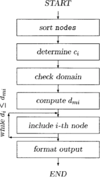
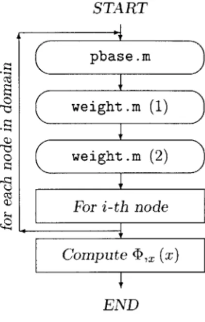
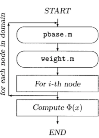
3.6.1 EFGM - DEM . . . . 3.6.2 EFGM - FEM . . . . 3.6.3 EFGM - hp Clouds . 3.6.4 EFGM - RKPM . . . . . 3.6.5 EFGM - SPH 4 Implementation 4.1 Introduction . . . . . 4.2 Program Description 4.2.1 process.m . 4.2.2 interior.m 4.2.3 lagrange.m . 4.2.4 pointforce.m 4.2.5 bodyforce.m 4.2.6 defdom.m . 4.2.7 dphi.m . . 8 38 38 39 40 43 43 44 44 44 45 47 47 48 49 50 50 50 51 51 53 53 53 54 55 56 56 56 56 57 . . . .
4.2.8 phi.m . . . .. . . . . 59 4.2.9 weight.m . . . . 59 4.2.10 pbase.m . . . . 59 4.2.11 gausstable.m . . . . .. . . . . 60 4.3 Program Input . . . .. . . . . 61 5 Computation 63 5.1 Introduction . . . . 63 5.2 Accuracy of Results . . . . 64
5.2.1 Numerical Patch Test . . . . 65
5.2.2 Point Force Applied in the M iddle . . . . 65
5.2.3 Effects of Discretization . . . . 66
5.3 Computational Effort . . . . 66
5.4 Variation of W eight Function . . . . 67
6 Conclusion 75 6.1 Summary . . . . 75
6.2 Results. . . . . 75
A Rod in Tension 77 A.1 Introduction . . . . 77
A.2 The Differential Equation of Equilibrium . . . . 77
A.2.1 Introduction . . . . 77
A.2.2 Fundamental Principles in Linearized Elasticity . . . . 77
A.3 The W eak Form . . . . 80
A.3.1 Introduction . . . . 80 A.3.2 Derivation . . . . 81 A.4 Discretization . . . . 85 A.4.1 Introduction . . . . 85 A.4.2 Formulation . . . . 86 9
B Numerical Examples 89
B .1 Introduction . . . . 89
B .2 Point Force . . . . 89
B.2.1 Point Force Applied at Tip . . . . 89
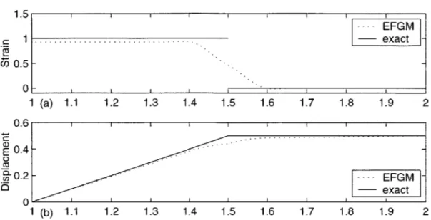
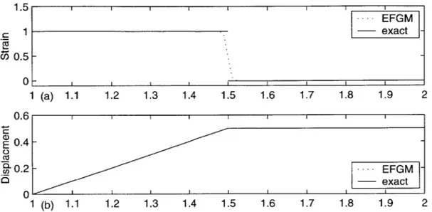
B.2.2 Point Force Applied in the Middle . . . . 94
B .3 Body Force . . . . 100
B.3.1 Constant Shape . . . . 100
B.3.2 Quadratic Shape . . . . 104
B.4 Comparison of Weight Functions . . . . 108
B.5 Weight Functions . . . . 111
Bibliography 115
Index 121
List of Figures
2-1 Interpolation of a function . . . . 2-2 Comparison of domains of influence.
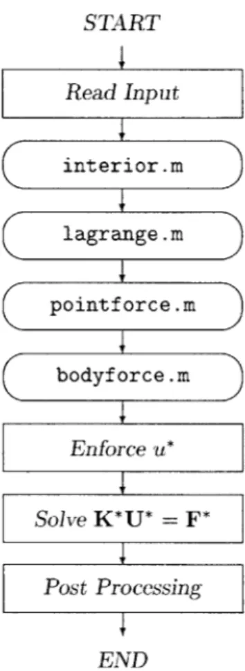
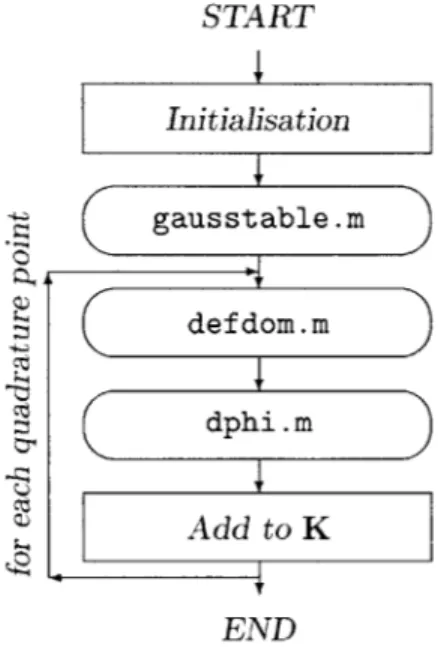
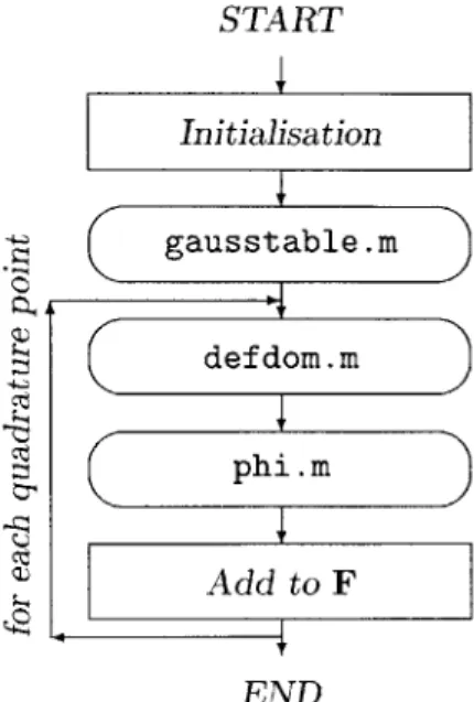
Flowchart of process.m . . . . Flowchart of interior.m . . . Flowchart of lagrange.m . . . Flowchart of pointf orce.m . . Flowchart of bodyf orce.m . . . Flowchart of def dom.m . . . . . Flowchart of dphi.m . . . . . . Flowchart of phi.m . . . . .
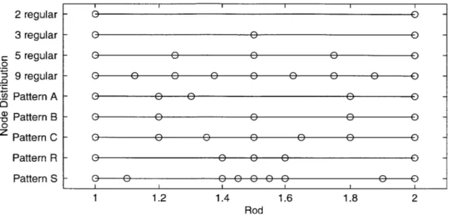
Employed node distributions . Results mid-located point force, Results mid-located point force, Results mid-located point force, Results mid-located point force, Results mid-located point force, Results mid-located point force,
3 nodes 3 nodes 3 nodes 3 nodes 9 nodes (regular), (regular), (regular), (regular), m 2 m=
3
m = 2, dfactor = 1.01 m = 2, dfactor= 3.0 4-1 4-2 4-3 4-4 4-5 4-6 4-7 4-8 5-1 5-2 5-3 5-4 5-5 5-6 5-7 5-8 5-9 5-10 5-11 5-12 5 nodes (Pattern R), m = 2 Results quadratic body force, 5 nodes (regular), m = 2 Results quadratic body force, 5 nodes (regular), m = 3 Results quadratic body force, 9 nodes (regular), m - 2 Results quadratic body force, 9 nodes (regular), m = 3 Results quadratic body force, 7 nodes (Pattern C), m = 211 . . . . 25 . . . . 29 . . . . 5 4 . . . . 5 5 . . . . 5 5 . . . . 5 6 . . . . 5 7 . . . . 5 8 . . . . 5 9 . . . . 6 0 . . . . 6 4 (regular), m 68 68 69 69 70 70 . . . 71 71 72 . . . 72 . . . 73
5-13 Results quadratic body force, 7 nodes (Pattern C), m = 3 . . . . 73
A-1 Rod, axially loaded . . . . 81
B-i Second order weight function by [30] . . . . 112
B-2 Fourth order weight function by [30] . . . . 112
B-3 Weight function by [20] . . . . 113
B-4 Weight function by [41] . . . . 113
List of Tables
B.1 Results end-point force, regular mesh . . . . 90
B.2 Results end-point force, irregular mesh . . . . 91
B.3 Results mid-located point force, regular mesh . . . . 94
B.4 Results mid-located point force, irregular mesh . . . . 96
B.5 Results constant body force, regular mesh . . . . 100
B.6 Results constant body force, irregular mesh . . . . 102
B.7 Results quadratic body force, regular mesh . . . . 104
B.8 Results quadratic body force, irregular mesh . . . . 106
B.9 Results with different weight functions: point force at tip, regular mesh . . 108
B.10 Results with different weight functions: mid-located point force, regular and irregular m esh . . . . 109
B.11 Results with different weight functions: quadratic body force, regular and irregular m esh . . . . 110
Notation
a2 Normalized weight in Gaussian quadrature
ogg
Kronecker deltaA Lagrange multiplier, Lame constant
p Lam6 constant
II Functional
<p Interpolation
/
approximation function<h(x) Moving Least Squares Interpolation functions
a(-,) Bilinear operator
a Interpolation
/
approximation coefficients A Cross section of rodA Matrix containing basis vectors p(xi)
A(x) Weighted moment matrix in Moving Least Squares Interpolation b Interpolation
/
approximation data pointsbo Body force vector
B(x) Weighted data points matrix in Moving Least Squares Interpolation 93 Domain of problem statement
So Interior of 93
ci Distance of most remote node in minimal domain of influence Cn Space of n times differentiable continuous functions
C Elasticity tensor
df actor Multplicator for domain of influence
dmi Radius of domain of influence of i-th node 89 Boundary of 9
E Young's modulus
E Infinitesimal strain tensor ch Strain energy of EFGM solution
f
Function to be interpolated/
approximatedfb Body force, in force per unit length
F Point force F Load vector
F* Load vector, amended by constraint u* G Shear modulus
G Constraint terms for essential boundary conditions yj2 Sobolev space
I Identity matrix K Stiffness matrix
K* Stiffness matrix, amended by constraint terms G
L Length of rod
LM Vector relating global and local node numbering 22 Space of square integrable functions
L2m Differential operator of order 2m m Order of basis vector p(x)
N Number of nodes
p(x) Basis vector in Moving Least Squares Interpolation P1 Space of linear polynomials
ri Normalized coordinate in Gaussian quadrature
r Residual
S First Piola-Kirchhoff stress tensor
SU Boundary of 9 with prescribed essential boundary conditions Sf Boundary of B with prescribed natural boundary conditions T Cauchy stress tensor
u* Prescribed displacement
u(x) Exact displacement solution U Nodal displacements
U* Nodal displacements vector, amended by Lagrange multiplier A v Test function
V Total solution space, including exact solution Vh Approximate solution space
V Vandermonde matrix
w(di) Weight function
W(x) Diagonal weight function matrix
Chapter 1
Introduction
1.1
Solution Methods for Field Problems
Solution methods for field problems are widely used mathematical tools in engineering analysis. These methods are applied in such areas as the anaysis of solids and structures, heat transfer, fluids and almost any other area of engineering analysis.
One of the best known and most widely used methods is the Finite Element Method, or FEM in short. Its first occurence, or the roots of its development, date back to over four decades ago [3]. Since then, significant changes have taken place. Nowadays, there seems to be almost no field in which the FEM is not present.
Much of the success of the FEM is due to its intuitively physical approach and its great versatility. Indeed, the FEM may be applied in almost any area, its underlying mathematical structure enabling widespread use.
But despite - or even because of - this generality, there are certain areas in engineering analysis that are not well suited for analyses by the FEM. One example is the area of fracture analysis. Even three dimensional dynamic crack growth may be simulated, but at rather high expenses. Remeshing, at least locally, is necessary and results in loss in accuracy and computational cost.
Recently, especially in the last decade, interest has grown in so-called meshless methods.
CHAPTER 1. INTRODUCTION
These methods are not based on the notion of an element, as in the FEM, but instead attempt to approximate the given geometry through other procedures. One of them is the Element Free Galerkin Method, or EFGM.
1.2
Meshless Methods
The area of research of meshless methods is in a developing state and much has been done already. An extensive, but already somewhat outdated review is given by Belytschko et al. in [6], which also mention the EFGM. The formulation of the EFGM is similar to that of the FEM in that it is based on a Galerkin weak form of the problem; however, instead of using fixed, local interpolants, it uses Moving Least Squares Interpolants.
1.3
Development of the EFGM
The name Element Free Galerkin Method was first coined by Belytschko et al. in [7]. It is an improvement of the diffuse element method, which was introduced by Nayroles et al. [34]. They did not note that the employed interpolants are in fact Moving Least Squares Interpolants, for example as studied in [30]. Belytschko et al. improved the diffuse element method significantly: accurate evaluation of the derivatives, high order of integration and exact enforcement of essential boundary conditions enabled the method to pass the patch test [7].
Since then, improvements to, and analyses of the method itself have been made (see Chapter 3). EFGM has been extensively applied to various field problems. The method performs especially well in the area of fracture analysis [8, 10, 32, 35, 36, 41], due to its dynamic connectivity of nodes. Further, it seems to exhibit no volumetric locking (provided appropriate basis functions are employed) [7, 28].
1.4. ABOUT THIS THESIS
1.4
About this Thesis
1.4.1
Intention
The objective of this research is to evaluate and examine the Element Free Galerkin Method. The method is applied to elastic rods subject to point forces and body forces. Its accuracy, characteristics and computational effort are examined.
1.4.2
Structure
The structure of this thesis is designed such that the EFGM is gradually developed. In Chapter 2 the fundamental utility in the EFGM is described, the Moving Least Squares Interpolants. Lagrange multipliers and numerical integration are mentioned, different math-ematical forms of the problem statement and error-distribution methods are reviewed.
Chapter 3 gives an introduction to the EFGM, describing its characteristics in dis-cretization, imposition of boundary conditions, numerical integration and post processing. Convergence of the method is mentioned with respect to the conforming and nonconform-ing EFGM. This Chapter closes with some relationships of the EFGM with other meshless
methods and the FEM.
Chapter 4 describes the implementation of the EFGM using Matlab for the case of elastic rods subject to point and body forces, imposing essential boundary conditions via Lagrange multipliers.
Chapter 5 reviews numerical examples computed with the Matlab routines and examines the accuracy of the obtained results. Further, some considerations with respect to different weight functions are given.
Chapter 6 discusses the results.
Appendix A develops the mathematical-mechanical background of the Matlab imple-mentation in Chapter 4. The amended weak form for a rod (essential for the EFGM employing Lagrange multipliers) is derived.
Appendix B tabulates numerical examples. Rods subject to point forces at the tip and in the middle and subject to constant and quadratic body forces are computed. In addition, 21
22 CHAPTER 1. INTRODUCTION
Chapter 2
Mathematical Background
2.1
Introduction
This chapter reviews some of the formulations and methods necessary for the Element Free Galerkin Method. The Moving Least Squares Interpolants are at the core of the method. These functions are gradually developed from the basics in interpolation.
Imposition of constraints by Lagrange multipliers is described, and some characteristics of numerical integration are mentioned. Different mathematical formulations of problems in elasticity are reviewed, including the weak form. The latter leads to error-distribution methods, including the Galerkin method.
2.2
Moving Least Squares Method
2.2.1 Introduction
In the following, interpolation and approximation by a polynomial is reviewed, leading to the method of Moving Least Squares Interpolation, which are interpolation functions with adjustable support. The more general case of multiple variables can be found in [30]. In the following only the one dimensional case is considered.
Note that:
CHAPTER 2. MATHEMATICAL BACKGROUND
* approximation in general is considered as the problem of representing some given function f(x) by some function
#(x),
which comes close in value but may not be exactly equal to f(x).e interpolation, roughly-speaking, denotes the approximate representation of some function f(x) in terms of N discrete data points (xi, f(xi)) and interpolation tions
#(X;
X1, X2, .. . , XN). In general, (; Xi, x2, - - - , XN) passes the value of"through" when being evaluated at x = xi, that is:
given
func-f (Xi)
#(xz;
1, X2, .. . , XN) = f (Xi) Vzi = 1, ... , N.Note, that eq. (2.1) is sometimes referred to as the interpolation condition, cf. eq. (3.1). When#(X;z, x2,.... , XN) does not satisfy eq. (2.1) exactly,
#(;
Xi, x2,... , XN) is therefore non-interpolating and resembles an approximation function.For ease of notation, in the following the dependency of
#
of Xi, x2,... , XN is omitted.2.2.2 Interpolation Using a Polynomial
An interpolation function approximates some given function by estimating its shape between discrete data points (later referred to as nodes).
In Figure 2-1 some given function
f
: D - R,f
() = y
(2.2)with discrete data points
(Xi, yi), f (Xi) = yi, i = 1,. .. N (2.3)
(2.1) 24
2.2. MOVING LEAST SQUARES METHOD 1 0.8- 0.6- 0.4-0.2 0 0 (a) Figure 1 0.8 -0.6 -0 x 0.4 0.2 1 0.8 0.6 -0.4 0.2 1 2 0 1 2 0 x (b) x (c)
2-1: Interpolation of (a) f(x) based on (b) two points 1
x
by (c) # (x)
2
is approximated by a line
#(x)
interpolating the given two data points. In general (for 2.2), 0#(x)=
p(x) a=ao +a1 x+ a2x 2+ - - -+ am-1 lm-1
a = (ao ai a2 ... am-1 , p x 2 ...
where the ai
C
R determine the shape of the interpolant. Note, that in the following p is said to be of order m = 2 when it contains at most the linear term: pT = (1 z).In order to obtain a unique linear interpolation, at least two independent points are required. For higher-order interpolating polynomials, obviously more data points are nec-essary to obtain unique interpolants. In general, N = m points are required to obtain a
unique polynomial of order m. with
(2.4)
(2.5) 25
CHAPTER 2. MATHEMATICAL BACKGROUND
Determining the interpolation function reduces to solving a system of equations. One may compute the coefficients a2 in eq. (2.4) by employing the Vandermondel matrix [2]:
Va = b, (2.6) where 1
1
V=
1
\1
£1 2 £1 1 2 £2 £2 2 X3 £3 2 £N £N ... £1 rn-1 ... £2 ''' 13 Xmi1 a / ao a, a2 Yi Y2 b= y3 \YN)2.2.3
Least Squares Approximation
Interpolation functions as presented in Section 2.2.2 are limited in applicability. In general,
N data points require the interpolating polynomial to be of order m = N. It is not possible to interpolate an arbitrary set of points by a polynomial of fixed order2. Mathematically,
the system of equations for N > m in eq. (2.6) is not solvable in general.
When the number of data points is high, approximation instead of interpolation is used. The function
#(x)
(to be determined) no longer interpolates the data points. For example, consider trend prediction and averaging in experimental data. Some error (called residual) in approximation is accepted.One method to obtain such approximations is the least squares approach3, where the error in interpolation at each data point is defined as:
ri q$) - yi, i=1,... ,N.
'Alexandre Th6ophile Vandermonde (1735-1796).
2
This is similar to a desk with four legs (data points) rocking on an uneven floor (interpolation function).
3
Problem definition and solution based on a method developed by Carl Friedrich GauB (1777-1855). (2.7)
2.2. MOVING LEAST SQUARES METHOD
The sum of these errors yields the residual of the approximation. In order to obtain the best approximation in the least squares sense (that means, minimizing the square of the residual) one has to determine the ai from eq. (2.4) such that
N
r 2 =11 r 12|= r'r
i=1
(2.8)
is minimized (11 - 112 is the Euclidean norm). Resorting to matrix notation, with:
1 1 1 \1 X1 x2 x3 XN ...
i-1
-.. 3 1 m X-1 -- N ao ai al , a= , b= Y21 y3 \YN/ (2.9)eq. (2.7) can be expressed as:
r = A a - b. (2.10)
Requiring rTr minimized leads to:
ATA a = ATb. (2.11)
Remark: Supposed, A E R(N,m) is of rank(A) = m, b E RN and N > m holds, then it can be shown that eq. (2.11) has a unique solution a E R" .
2.2.4 Moving Least Squares Interpolation
Least squares approximation, as described in Section 2.2.3, minimizes the square of the residual over the whole set of data points (Xi,y 2), i 1,... , N, equally weighted4. The
4
The interpolation functions span the whole domain. Note the similarity to the Standard Ritz Method, which spans over the whole region - in opposite to the Finite Element Method.
CHAPTER 2. MATHEMATICAL BACKGROUND
approximating curve spans over the whole domain, or set of (xi, yt). It loses local accuracy. However, loss in accuracy, and wide-spanned domains may be circumvented by introducing localization terms in eq. (2.11).
Consider in eq. (2.11), instead of the moment matrix ATA, some weighted matrix product:
ATW(x)A a(x) = ATW(x)b, (2.12)
with W(x) a diagonal matrix with N weight functions:
Wij (x) = w(di)
o1-,
(2.13)and a(x) the coefficients of the approximation function, as before. Note that both terms W(x) and a(x) are functions of x, while A, similar to the Vandermonde matrix, is a quasi-constant matrix storing the basis vectors p(xi) of nodes with nonzero weights, cf. eqs. (2.15, 2.24). The weight functions in W(x) limit the influence of its nodes to the corresponding domain of influence.
When computed by eq. (2.12), the coefficients ai(x) are not constant, as in eq. (2.4). Instead, they change continuously over the whole domain, introducing the localized weight of W(x) in the definition of
#b(x).
Note that due to the localization of the interpolation,multiple interpolation functions exist, one interpolation function for each data point xi. Eq. (2.12) is the definition of the Moving Least Squares Interpolant (or approximating function) in one dimension5. The derivation for the general case may be found in [30].
Weight Function and Domain of Influence
The localization term W(x), defined in eq. (2.13), distinguishes the Moving Least Squares Method from the standard least squares method. The choice of the weight function and
5
Note, that Moving Least Squares Interpolation implies the notion of the support moving with the evaluation point x.
2.2. MoVING LEAST SQUARES METHOD 29
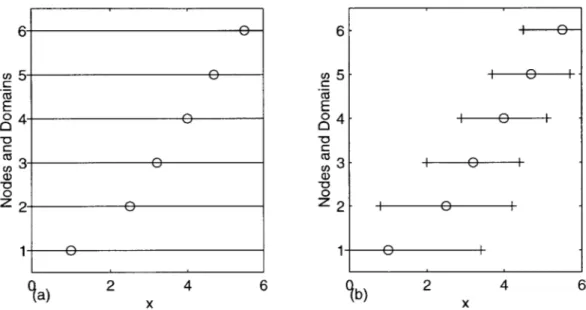
the definition of the domain of influence is an important part in Moving Least Squares Interpolation. 6- E) 6-
e
cnO e 5 I-E E 04 e 04 0 4 1 010 I a ) a ) 0 0 2-
p z 2e
ja) 2 X 4 6 c b) 2 X 4 6Figure 2-2: Domains of influence in (a) least squares approximation, (b) Moving Least Squares Approximation
The size of the domain of influence is determined by the definition of the weight function. Constant weight functions, which have unit value over the whole domain, yield the regular least squares approximation. Smooth weight functions with circular domains6 and limited radius are employed in general. The circular domain (or in three dimensions: the ball-shaped domain) degenerates for one dimension to a line, where the weight function of the i-th node may be defined as:
Jw(di) if di < dmi, w (di) =(2.14)
0 if
di
> dmi,with dmi the radius of the domain of influence [7] and di the distance of the i-th node
6
CHAPTER 2. MATHEMATICAL BACKGROUND
from the evaluation point x:
di =
Ix
- xi|.It is important that the domain of influence is chosen such that ATW(x)A is not a singular matrix. This requires that at least m nodes have nonzero weights. The process of determining the domain of influence (di varies in general with x and is not constant for irregular meshes) consists of the following steps:
" determine some ci defining the distance di of the most remote node in the domain for a minimum set of nodes,
* enlarge this minimum domain by defining dmi = df actor ci, where df actor may be chosen to be 1 and higher7. With dfactor
= 1, piecewise linear interpolants are obtained, leading to the linear FEM as a special case of the EFGM [36]. Note that values
dfactor > 3 may yield too smooth interpolants, leading to underestimation of results.
Moving Least Squares Interpolants may be interpolating and non-interpolating, depend-ing on whether the weight function is sdepend-ingular at x = x,. In general, the non-interpolatdepend-ing version is employed.
Some weight functions used for Moving Least Squares Interpolants are given in Ap-pendix B. Note the difference between the singular weight functions in Figures B-1 and B-2 by Lancaster et al. [30] and the smooth weight functions in Figures B-3 and B-4, re-spectively, by [20, 41]. Employing the latter gives non-interpolating Moving Least Squares Interpolants, while using the singular weight functions yields interpolating Moving Least Squares functions. Note that the singularity requires some attention in numerical methods.
7
Organ [36] recommended dfactor values (denoted as da,) ranging from 2.01 to 2.51, while Belytschko et al. mentioned 2.0 < df actor < 3.0 for elastodynamics [8].
2.2. MOVING LEAST SQUARES METHOD
Formulation
It should be noted that the Moving Least Squares Interpolants are not polynomials, but rational functions. Furthermore, due to the complexity,
#i(x)
may not be computed analyt-ically. One has to resort to numerical evaluation of the interpolants at the required points. For the case of the interpolant#i(x)
itself, a (x) has to be computed from eq. (2.12). That is, a set of linear equations has to be solved.To obtain dP"(x) -
#i,x(x),
some attention may be required. Employing the followingdefinitions:
A(x) = ATW(x)A, (2.15)
B(x) = ATW(x), (2.16)
U = b,
where U contains the nodal unknowns, one arrives at the definition of the Moving Least Squares interpolants for the EFGM. The basic approach is similar to eq. (2.4), where the analytical solution u(x) is approximated as follows:
u(X) 4(x) U = pT(x) a(x), (2.17)
u(x(x) ~ ,x(x) U = p T (x) a(x) + pT(x) a,x (x), (2.18)
where
a(x) = -1 (x)
5(x)
U, (2.19)a,(X) = (A1(x) (x) + k (x)
5,(X))
U.Avoiding the computationally intensive term A,- (x) leads to:
a,X(x) =( - (x) ,(x) A-1(x) S(x) + A1 (x) 5,i(X) U. (2.20)
CHAPTER 2. MATHEMATICAL BACKGROUND
The shape functions (and its derivatives) for the EFGM may be computed from eqs. (2.17, 2.18) by substition of eqs. (2.19, 2.20), respectively.
Note that:
* the dimensions of the matrices are
A(
E
R) R(m,") and B(x) E R(mN), where m denotes the order of the basis vector p(x) and N is the number of nodes, which weights are nonzero. For one dimensional problems choices for p(x) are:P
=(1
X),
m = 2, (2.21)pT = x x2), m = 3, (2.22)
pTWx =
(1
x 2 X 3), m= 4, (2.23) etc.* In the routines in Sections 4.2.7 and 4.2.8 A(x),
N(x),
A,x(x)
andN,x(x)
are com-puted as follows:N
A
(x) = w (di) p (xi) pTMx) ( 224N(z)
= (w(di) p(zi) w(d2) p(X2) ... w(dN) p(zN) , (2.25)N
AI(x) = w,x (di) p(xi) pT(zi), (2.26)
Bx(X) =
(w,(di)
p(xi) w,x(d2) p(X2) ... w,x(dN) P(XN)) (2.27)2.3
Lagrange Multiplier
The method of Lagrange8 multipliers is a convenient way to solve problems subject to some given constraints. As an example, consider the problem of obtainig stationary values of
8
Joseph Louis Lagrange (1736-1813).
33 2.3. LAGRANGE MULTIPLIER some function f (x), x C R7: Of df =
dx
1+
Oxisubject to the two constraints
ci(x) 0,
c2(x) = 0.
By amending f(x) with the given constraints:
f*= f
+ Ai ci =f + A1 ci + A2 c2and taking the variation of
f*
yields:Of + A, Oci
Oxi Oxi
0c2
+A 2 =0
Oxi
Note that the conditions in (2.31) are the conditions of
f*
be stationary [21].To show that eq. (2.31) is in fact equivalent to eq. (2.28), subject to eqs. (2.29, 2.30), consider the following relations:
i=1
0ci dxi = 0,
Oc2 dxi = 0.
(2.32)
(2.33)
They follow directly from eqs. (2.29, 2.30). Multiplying eqs. (2.32, 2.33) by A1 and A2, respectively, and adding both equations to eq. (2.28) gives:
±Of i=1 x1 + A1 + A2 dzi = 0. Oxi Ox2)d 1 0 (2.34) Of Ox dX2 2 822 Of -+- + dx 1, = 0 Oxn (2.28) (2.29) (2.30) Vi = 1, ,n. (2.31)
CHAPTER 2. MATHEMATICAL BACKGROUND
From eq. (2.34), it can be seen that eq. (2.31) indeed holds. In general, the method of Lagrange multipliers may be used with more than two terms.
In Section A.3.2 Lagrange multipliers are employed to impose essential boundary con-ditions.
2.4
Numerical Integration
Numerical integration (in the following only for the case of one dimension) is the process of approximately integrating some function numerically, that is, based on the function itself instead of the analytical expression of F =
f
f
dx. For example, one basic method isSimpson's Rule.
The most widely-used method of numerical integration is Gaussian quadrature, but as mentioned in [37], in some cases even more accurate formulas with less sampling points have been developed. In Gaussian quadrature polynomials
#(x),
as defined in eq. (2.4), may be integrated exactly, provided the required number of sampling points (sometimes called Gauss stations) is used.The basic assumption in Gaussian numerical integration is that the integral can be approximated by a finite number of weighted sampling points:
b
If
(x) dx = w1 f (xI) + w2 f (x2) + ... + w,f
(x,) + Ry, (2.35) awhere the last term, R., is the error in the approximation.
Consider some polynomial,
#(x),
xC
R, as defined in eq. (2.4). It can be shown, that polynomials of order (2p - 1) are integrated exactly, provided p sampling points are used[3]:
b
#(x) dx = wi#(xi). (2.36)
a i
2.5. PROBLEM FORMULATION
Eq. (2.35) is not used in practice. Instead, the weights and sampling points are transformed to normalized representation, based on the following expressions:
b m
f
(x) dx ~wif (xi), (2.37) a j: a+b b-a X = + r, r E [-1; 1] (2.38) 2 2 wi = b -a ci. (2.39)The sampling points r. may be determined employing the Legendre-Polynomial [2]. An extensive collection of sampling points and weights may be found in [1].
So far only integration of polynomials is considered. However, rational, or nonpolyno-mial functions may be integrated using Gaussian quadrature. Obviously, no exact results are obtained, only approximations. Section 3.3 deals with the accuracy in integration of rational functions, like Moving Least Squares Approximations.
2.5
Problem Formulation
The following Sections are concerned with the various formulations and expressions which are involved in processes such as the development of the weak form as in the Appendix A or the convergence of the EFGM itself [29]. Most of the following departs from the well-known statement in eq. (2.40).
2.5.1 Differential Form
Consider some given boundary value problem. For the sake of simplicity, only one dimen-sional problems in the region 93
{
x 10 < x < L}
are considered:d
duia
dEA d
+fb=0 (2.40)dx ( dx
where the displacements are prescribed on Su and tractions
/
forces act on Sf.CHAPTER 2. MATHEMATICAL BACKGROUND
Note that boundary conditions in general may be distinguished by the order of their differential operations [24], where 2m is the order of the differential operator in eq. (2.41):
*
0 ... m - 1: essential, geometric or Dirchlet boundaries,* m ... 2m - 1: natural, additional or Neumann boundaries.
2.5.2 Operational Form
The differential form of eq. (2.40) may be formulated as follows [37]: Find a unique corre-spondence, that is, find some relation between some given inhomgeneous term
f
and someu for the region B, each of them members of some spaces of functions, which satisfies the
given differential equation and boundary conditions.
This process of matching spaces of functions is generally written by using differential operators:
L2mU=
f
in the region B C R, (2.41)where L2m is a differential operator of order9 2m which in general establishes a unique one-to-one mapping of some
f
to someu.
L2m acts on a certain class of functions - those which in some sense satisfy the boundary conditions, prescribed on 93 = S, U Sf, and which can be differentiated 2m-th times (denoted as C2m functions).Note that eq. (2.41) is the Euler10 equation.
Consider the class of admissible functions of u and
f.
Onlyf
with finite energy are admitted:(f) 2 dx < oc. (2.42)
In this case, the integral expression in eq. (2.42) is the square sum over all body forces applied to the rod, therefore it is reasonable to require this integral to be finite. The space
9
1f not otherwise mentioned, the order of the differential operator is 2m = 2.
'0Leonhard Euler (1707-1783).
2.5. PROBLEM FORMULATION
of functions which satisfy eq. (2.42) is often denoted Z2, which here is defined as:
2 =
{w
I
w defined in M andf
(W)2dV < oo}. (2.43) MIt follows that the space of admissible functions for eq. (2.41) is the Sobolev space 5f.
That is, where: (1) the interpolation function, (2) its first derivatives and (3) its second derivatives are required to be in Z2 [22, p. 267]. Obviously, only functions in 552 are allowed
which satisfy the given boundary conditions.
Once these requirements on u and
f
are satisfied, and L2m is in fact a one-to-one transformationil, it can be shown that the given boundary-value problem has a unique solution u. Physically, the existence of a unique u for the operator L2m expresses the following: For a problem within the linearized theory of elasticity there exists one unique deformed shape u for each loadf.
2.5.3 Variational Form
An alternative form to the statements in Sections 2.5.1 and 2.5.2 is the variational form. Consider eq. (2.40), weighted by test functions v and integrated over the domain T12:
a(L2m,) = a(f, v) for every v. (2.44)
This equation is the result of varying the quadratic I(v) = a(L2mo, v) - 2 a(f, v), that is
minimizing 1(v).
Note that due to integration by parts, eq. (2.44) does not contain second derivatives of u, see eq. (A.15). In fact, the space of admissible solutions in the minimization is 551, where
the functions are only required to satisfy the essential boundary conditions in advance. The fundamental enlargement of admissible functions to piecewise linear C0 -continuous
"This requires L2m to be self-adjoint and positive definite.
1 2
Here a(., -) is a bilinear form corresponding to the considered model problem. "Bilinear" denotes that this form is linear in both elements on which it operates.
CHAPTER 2. MATHEMATICAL BACKGROUND
functions1 3 enables, for example, the use of two-node elements in elasticity problems in the Finite Element Method.
In EFGM this enlargement by piecewise linear C0-continuous functions of the space of admissible functions is not necessary. However, the admissible functions have to satisfy the essential boundary conditions. This is not satisfied in general by the interpolation functions employed in EFGM, the Moving Least Squares Interpolants.
2.6
Method of Weighted Residuals
2.6.1 Introduction
The method of weighted residuals seeks to determine a best approximate solution to a differ-ential equation, subject to boundary conditions, through the use of trial (and test) functions [11]. It focuses on the error in satisfying the given problem, similar to the interpolation in Section 2.2.3.
Error-distribution methods yield results which in some sense are the best approximations to the exact solution. Different methods are available [11], where T = 8T + 9a, so that 8% denotes the boundary and 9o is the interior of 93:
" boundary method: The differential equation is satisfied exactly in the interior 90, and the unknowns are selected to fit the boundary conditions in some best sense.
" interior method: The trial functions are chosen such that they satisfy the boundary conditions exactly, and the residual is minimized over the whole interior 9o.
* mixed method: Neither the differential equation in 30, nor the boundary conditions
on &Z are satisfied. Here, the unknowns to be determined are selected to satisfy both the differential equation and the boundary condition in some best sense.
13
Slope discontinuity allowed, but discontinuities in u itself prohibited.
2.6. METHOD OF WEIGHTED RESIDUALS
2.6.2
Formulation
Given some problem statement, cf. eq. (2.41):
L2 mU -f = 0 in the region
9
(2.45)with boundary conditions prescribed on 8o = Su U Sf. Consider the following approach by the interior method: Some approximate solution of the differential equation is assumed:
N
Uu '-
Z
qOi W ui, i=1where the ui are the unknowns to be determined, and the
#j(x)
are trial functions which are chosen to satisfy all boundary conditions. This approximation, employed in eq. (2.45), is not likely to satisfy the differential equation exactly. Some error, called residual, remains:r(x) = L2mii -
f.
This residual is required to vanish or being minimized over the interior 9o, appropriately weighted by test functions14:
Jvi(x) r (x) dxO = 0, Vi = 1, ... , N, (2.46)
where the vi(x) are N linearly independent functions. The exact solution is obtained if eq. (2.46) holds for any complete set of functions v,(z), with N -* oc. In practice, only a
limited number of functions is chosen.
The various choices of test (or weight) functions gave birth to several methods within the class of error-distribution methods. In the following, some widely-used methods are described.
"In [13], r(x) is said to be orthogonalized to vi(x) over the interior o.
CHAPTER 2. MATHEMATICAL BACKGROUND
2.6.3 The Galerkin Method and other Error-Distribution Methods
Next to the Galerkin method1 5
, which is "the obvious discretization of the weak form" [37,
p. 117]16, other error-distribution methods have been established and used.
Collocation Method
In the collocation method1 7 the residual is required to vanish at N
points. That is, the
vi(x) are chosen to be the Dirac delta function 6(x-xi). However, the approximate solution
does not coincide at the points xi with the exact solution [24]. Furthermore, the obtained results may fluctuate widely between the xi [11].
Least Squares Method
This method was first mentioned by Picone in 1928 [18]. Here, the integral of the square of the residual is not forced to be zero, but instead required to be a minimum with respect to the unknown ui. However, the involved integrations may often be complicated [21].
Subdomain Method
In the subdomain18 or partition method the region is divided in subdomains. The integral of the residual is required to be zero over each subdomain. Hence, the weight functions may be considered unit step functions, which are unity in the
i-th
domain and zero elsewhere.Galerkin Method
In the Galerkin method the test functions vi(x) are chosen to be the trial functions
#j(x)
themselves. That is, the residual is forced to be orthogonal to the space of trial functions. Strang and Fix [37] expressed Galerkin's rule as follows (note that the approximate solution space Vh, determined by the interpolation functions, is denoted Sh, where ii E Sh):1 5
Boris Grigorewitsch Galerkin (1871-1945) mentioned this method in 1915 [18].
16
Note that eq. (2.45) is the differential form, or strong form, and not the weak form.
1 7
First mentioned in 1937 by Frazer, Jones and Skan [18].
1 8
Finlayson et al. [18] name Biezeno and Koch as the first to mention this method in 1923. 40
2.6. METHOD OF WEIGHTED RESIDUALS 41
The residual Lu-f will not be identically zero unless the true solution u happens to lie in the trial space Sh, but its components in Sh should vanish.
Chapter 3
Element Free Galerkin Method
3.1
Introduction
This Chapter describes the characteristics of the Element Free Galerkin Method and gives an overview of the EFGM and some already examined features.
The Element Free Galerkin Method is a numerical method for approximate analysis. Some notes on its development are given in Section 1.3. Descriptions of the EFGM may be found in most of the publications named in the Bibliography. It should be noted that the area of research of meshless methods, and therefore of the EFGM, is steadily developing. The following descriptions do not claim to be "state of the art" or "cutting edge". But they may be satisfactory as an introductory approach to the EFGM, mentioning limitations without lacking reasonable accuracy and some actuality. The reader may miss some of the mathematical notation. This is outlined in parts in Chapter 2 and not repeated here. Additionally, Appendix A describes the complete derivation of the formulation for an elastic rod.
Possibly the most significant drawback of the EFGM is that the computational effort is high, the method is expensive. But the whole area of meshless numerical methods is still developing, and when considering the computational effort spent on Finite Element Analyses with millions or more degrees of freedom, this disadvantage may fade in future.
CHAPTER 3. ELEMENT FREE GALERKIN METHOD
3.2
Discretization and Boundary Conditions
As in all meshless methods, the difficulties arising from essential boundary conditions are directly related to the interpolation functions [25, 29]. Moving Least Squares Interpolants are generally employed in the EFGM, which directly affect the process of meshing.
3.2.1 Meshing
The EFGM belongs to the class of so-called meshless methods. That is, there exists no consideration of elements as in the FEM. The region of the field problem, 9, is not required to be subdivided into separate cells, or elements. The procedure of "meshing" reduces -in the pure sense of a meshless method - to distributing nodes in an arbitrary shape over the domain
The difficulties in meshing, and especially, in remeshing2
, are avoided. For example, even adaptive schemes (variable node density based on interpolation error estimation) have been developed to automate and accelerate the solution of some time dependent problems
[20].
3.2.2 Shape Functions
In the EFGM in general Moving Least Squares Interpolants are employed as shape functions (also called interpolation functions).
They span the space of discrete solutions Vh (note that V denotes the total solution space, including the exact solution). Alternatives or modifications may be used, like pseudo-derivatives of Shepard functions [26] or modified Moving Least Squares Interpolants with orthogonalized basis functions [31]. Even accelerated computation of derivatives [5} and enrichment of the basis to improve the representation of crack tip fields have been developed
'Obviously, the density of nodes should be based on the expected field solution.
2
For example, remeshing is of importance in field problems with time-dependent domains, that is, chang-ing geometry. This advantage explains much of the success of the EFGM in the area of fracture analysis
3.2. DISCRETIZATION AND BOUNDARY CONDITIONS
[40]. In this thesis Moving Least Squares Interpolants, as described in Section 2.2, are employed.
Moving Least Squares Interpolants are superior to finite element shape functions with respect to adaptivity. Nodal connectivity is not defined in advance, but may change to-gether with the geometry. Nodes may also be added and subtracted from the region quite easily. This advantage comes along with the disadvantage of high computational cost in evaluating the shape functions at the quadrature points3. Another drawback, next to this computational burden, is the loss of the physical meaning of the nodal unknowns4. The displacement at node i does not represent the displacement at this location . As mentioned in Section 2.2.4, Moving Least Squares Interpolants, as used in the EFGM, do not satisfy the interpolation condition:
Oi(zj) 6ij. (3.1)
Instead:
N
u(Xi) = #3 Oj(Xi) Uj # Ui. (3.2)
j=1
This disadvantage affects the imposition of boundary conditions.
3.2.3 Imposition of Constraints
Approximation functions used in the weak form are required to satisfy the essential bound-ary conditions. Similar to the principle of virtual work, the virtual displacement has to vanish at supports, while natural boundary conditions do not have to be satisfied in ad-vance.
3
Noted in Section 2.2.4, a linear set of equations (2.17, 2.18) has to be solved for each evaluation point.
4As long as non-singular weight functions are employed (which is recommended, since the singularity
imposes certain difficulties in the numerical implementation of the interpolants), the interpolation condition is not satisfied.
CHAPTER 3. ELEMENT FREE GALERKIN METHOD
Essential Boundary Conditions
Essential boundary conditions, which are prescribed displacements, have to be satisfied in advance by the approximation functions. As in other meshless methods, this requirement is not satisfied exactly by the Moving Least Squares Interpolants, as long as no additional constraints are present. In the EFGM, prescribed displacements may not be imposed di-rectly on the system of equations, for example by eliminating rows and columns, or by the penalty method. Instead, Lagrange multipliers [7] , coupling with finite elements [25, 38, 39] or modified variational formulations [31] have to be used. Note that the accurate enforce-ment of essential boundary conditions is one of the differences between the Diffuse Eleenforce-ment Method and the EFGM.
In this thesis, for the one dimensional case, Lagrange multipliers are used to satisfy essential boundary conditions. For problems with increased complexity, coupling of EFGM with FEM domains using ramp functions should be used to avoid the difficulties arising from essential boundary conditions acting on meshless domains.
Natural Boundary Conditions
Natural boundary conditions, like tractions in the case of elasticity problems, do not have to be satisfied in advance by the shape functions (in opposition to essential boundary conditions). The process of obtaining the best approximate solution employing the weak form of the given problem includes already the imposed natural boundary conditions.
Note, that in the case of point forces , some considerations on the accurate formulation are necessary. A point load may be seen as some distributed load with the Dirac delta function as weight function [23]. Suppose within some EFGM discretization, the source point of a point load may coincide with the position of a node. Still the point force has to be distributed using Moving Least Squares Interpolants.
3.3. INTEGRATION
3.3
Integration
The underlying error-distribution method in EFGM is the Galerkin method. Integration is an essential part in Galerkin methods, but it increases the computational burden.
Integration in meshless methods, as in the EFGM, may be some source of confusion. Despite its meshless character, there exists in EFGM at least some subdivision of the domain required for integration. These integration cells, also called background mesh, however, are in general not related to the nodal distribution [7]. But there exist implementations which connect the quadrature cells to the nodes [41].
Integration in the EFGM is performed numerically. In general, Gaussian integration is used. But determining the required order of integration is not as straightforward as in the FEM. In FEM, there exist exact definitions of the terms "full" and "reduced integration", and one can easily determine the required amount of quadrature points for full integration. As mentioned in Section 2.2.4, the interpolation functions in the EFGM are rational, and therefore cannot be integrated exactly. Still, numerical integration is sufficient, as long as the error in integration is small enough not to deteriorate convergence. The effects of integration on accuracy and convergence have been mentioned [16, 17]. For a too low order of integration, meaningless (oscillating) results were obtained (see also Appendix B).
Attempting to reduce the computational cost of integration, Beissel and Belytschko implemented a nodal integration scheme of the EFGM, but failed for the case of the unsta-bilized form [4].
3.4
Post Processing
As noted in [7], the EFGM relaxes the requirements on smoothing of results during post processing. The highly smooth Moving Least Squares Interpolants do not exhibit any jump discontinuities (as it is the case in the FEM with linear shape functions) in derivatives, not considering fracture analysis.
However, since the Moving Least Squares Interpolants do not satisfy the interpolation 47
CHAPTER 3. ELEMENT FREE GALERKIN METHOD
condition (see eq. (3.1) in Section 3.2.2), the solution U lacks some physical meaning. In order to obtain the smoothed interpolated solution <b(x)U, the Moving Least Squares Interpolants have to be evaluated. Again, as in the integration process, this increases computational cost.
3.5
Convergence
Convergence of the EFGM may be shown as in [37, p. 18] for the FEM:
Consistency and stability imply convergence.
Krysl and Belytschko adapted some of Strang and Fix's approach in [29].
From a less mathematical point of view, Hughes' notes of the requirements on shape functions for convergence in FEM may be considered [22]. The shape functions are required to be:
" smooth (at least C') on each element interior, " continuous across each element boundary and
" complete.
Not all three requirements are directly applicable. One of them is satisfied in advance, the smoothness criterion5. The completeness criterion, however, requires more attention:
Completeness requires that the rigid body displacements and constant strain states be possible. [3, p. 377]
Completeness requires that the element interpolation function is capable of ex-actly representing an arbitrary linear polynomial when the nodal degrees of freedom are assigned values in accordance with it. [22, p. 111]
5
Note that in fracture analysis the discontinuous shape functions, constructed by the visibility criterion [8, 10, 29] do not satisfy this requirement in advance. However, this study is not concerned with fracture
analysis, and therefore, the interpolation functions are smooth over the entire domain. 48
3.6. RELATIONS OF FIELD SOLUTION METHODS
That is: an element / mesh / discretization must exactly represent all rigid motions (rigid translations and rotations) and constant strain states. Both descriptions of completeness6 are formulated for the FEM, but are also applicable to the EFGM.
Patch Test
A well-known (but in its numerical implementation not sufficient) test for completeness is the patch test. Krysl and Belytschko showed the following [29]:
a(ii, dj) = a (ii, #i),
where a is the analytical bilinear operator, ah the discrete operator (the EFGM formulation),
4 as again the Moving Least Squares Interpolants and ii any arbitrary linear polynomial:
ii E P1 , Pi ={ pp = co
+
ci x, co, ci const. E RIRigid motions may be represented in this case with ci = 0, while the constant strain state requires ci : 0.
In [29] it is shown that for the case of discontinuous shape functions (see Section 3.5) this requirement is only satisfied in the limit, but it is said that convergence is demonstrated. Continuous shape functions, however, though being rational, can interpolate polynomials of certain order exactly. See Belytschko et al. [7] and Nayroles et al. [34].
3.6
Relations of Field Solution Methods
Without any intention of completeness, some relationships within the area of approximate field solution methods are described.
6Note, that the term "consistency" is equivalent to "completeness" [37, p. 175].