Analysis of certain inviscid flows on the beta plane

ANALYSIS OF CERTAIN INVISCID FLOWS ON THE BETA PLANE

by Boris Moro

SUBMITTED IN PARTIAL FULFILLMENT

OF THE REQUIREMENTS OF THE DEGREE OF

DOCTOR OF PHILOSOPHY

at the

MASSACHUSETTS INSTITUTE OF TECHNOLOGY

and the

WOODS HOLE OCEANOGRAPHIC INSTITUTION

January 1986

@ Massachusetts Institute of Technology 1986

Signature of Author_

Massachusetts Institute of Technology

-Certified by

I-Joint Program in Oceanography Woods Hole Oceanogranliic Institution

Steven A. Orszag Thesis Supervisor Accepted by___

A e bJoseph Pedlosky

Chairman, Joint Committee for Physical Oceanography

IT7

H

K~ST FEj

-2-ANALYSIS OF CERTAIN INVISCID FLOWS ON THE BETA-PLANE

by BORIS MORO

Submitted to the Department of Earth,Atmospheric and Planetary Sciences

on January 22, 1986 in partial fulfillment of the requirements for the Degree of Doctor of Philosophy

ABSTRACT

An investigation of properties of the solutions of the steady state inviscid quasigeostrophic vorticity equation in a rectangular basin, was performed for various assumed functional relationships between potential vorticity and the streamfunction. All solutions that were found, which have slow interior flow and satisfy the Arnol'd-Blumen condition, are qual-itatively similar to Fofonoff's inertial gyre. A new class of solutions with a small vortex near the boundary current is described. Such solutions are not stable under finite amplitude perturbations, but the vortices have life-time much longer than their characteristic life-time. The relationship between bottom friction and wind forcing and the westward motion of vortices is established. It is shown that friction may act as a mechanism for conver-sion of kinetic energy of rotation into kinetic energy of translation. It is argued that friction may be among the causes of westward motion of the mesoscale eddies. It is also shown that the inertial boundary current may be much wider than in Fofonoff's model, due to the appearance of a coun-tercurrent on its seaward side.

Several solutions describing steady general circulation in two layer model are found. We discuss strongly baroclinic long living vortices and a pure baroclinic mode of general circulation.

A simple approach to the numerical solution of some systems of

nonlinear elliptic partial differential equations, depending on several parameters is also described.

Thesis Supervisor: Dr. Steven A. Orszag

Title: Professor of Applied and Computational Mathematics Princeton University

-3-ACKNOWLEDGEMENTS

Author is indebted to Drs. N.P. Fofonoff and J. Pedlosky for useful sugges-tions, and to Prof. S.A. Orszag for support and encouragement. Computa-tions were performed on computers of the National Center for Atmos-pheric Research*. I should also like to acknowledge support under ONR contract 150F090 and NSF grant ATM 84-14410.

* The National Center for Atmospheric Research is supported by the National Science Foundation.

-4-CONTENTS

I Introduction 5

II Barotropic Flows

1 Steady State Solutions 17

2 Perturbation Experiments 33

3 Influence of Friction 48

4 Influence of the Wind Stress 68

III Two Layer Flows

1 Numerical Method 88

2 Mixed Modes 96

3 Evolution Experiments 110

4 Pure Baroclinic Mode 126

IV Conclusions 137

V Appendix

Numerical Solution of the

Quasigeostrophic Vorticity Equation

in Two-Layer Model 142

-5-I INTRODUCTION

The thesis is concerned with some problems of general circulation and its relation to mesoscale flows. We shall first review previous theories. New results are presented in Chapter II, which deals with barotropic flows, and Chapter III where baroclinic flows are discussed. Some suggestions about possible generalizations and future work are given in Chapter IV.

The earliest models of steady, homogeneous, large scale circulation, developed by Stommel and Munk, succeeded in explaining some of the basic features of the oceanic circulation, in particular showing that the reason for the existence of the intense western boundary current is the variation of the Coriolis parameter with latitude. In both Stommel's and Munk's models steady state solutions were obtained assuming linear dynamics in which the energy of the wind stress is absorbed in the basin and dissipated in the western boundary current. Advection terms were neglected, which is a good approximation in the interior of the basin. How-ever in the region of the boundary current, these terms can be neglected only if the friction is assumed to be unrealistically large. Although, the solutions included strong western boundary current, the dynamics of the intensification remained unclear. Pedlosky (1965) gave a simple explana-tion in terms of Rossby waves which display strong anisotropy in east-west energy transmission, caused by the 8-effect. From the dispersion relation for Rossby waves, it can be shown that energy associated with large scales must be transmitted to the west, and will be reflected with reduced wavelength, thus making the western boundary a source of small scale

-6-energy which is then dissipated in the viscous boundary layer. As in the models of Stommel and Munk, this theory is limited to the small ampli-tude motions (note that one plane Rossby wave is the finite ampliampli-tude solution of the vorticity equation, but a wave packet is not). This poses the question whether there are low frequency but large amplitude motions which will show similar behavior.

In large scale circulation (e.g. in the North Atlantic subtropical gyre (Fig 1.)), the observed boundary current transport is several times larger than the transport of the interior, wind-forced flow. This shows that for a more accurate description of the general circulation nonlinear effects must be taken into account.

While Stommel and Munk obtained solutions of the equations of motion by neglecting nonlinear terms, Fofonoff (1954) considered steady flow without forcing and friction, i.e. when the flow is described only by the advection of potential vorticity. In this case the barotropic vorticity equation reduces to the functional relationship between potential vorticity and the streamfunction. By assuming the dependence to be linear,

Fofonoff was able to find an analytic solution which consists of slow inte-rior westward flow and a fast eastward current at northern and/or south-ern boundary (Fig. 2). From the form the simplified equation of motion, it is clear that such solutions must have east-west symmetry, which is bro-ken either by friction, or by variations in the bottom topography.

-7-Figure 1. The North Atlantic Subtropical Gyre (Worthington, 1976)

COmuz rm @.0000 to 0.00006 COu INEVA, Or 0.10000 PZ(3,3). 0.637M-02

-8-Merkine et al. (1985) argued that such a "linear" model is barotropi-cally unstable, although it can be shown that it satisfies the sufficient con-dition for stability in inviscid fluid under small but finite amplitude per-turbations due to Arnol'd (1965) and Blumen (1968). This flow pattern is often regarded as a peculiarity of the linear relation between the potential vorticity and the streamfunction. Pierrehumbert and Malguzzi (1985) con-sidered an essentially inertial ocean with forcing and dissipation included as higher order effects. By making an expansion of the streamfunction in terms of a small parameter which determined the size of the sources and sinks of energy, they derived a system of nonlinear integro-differential equations, one of which, in principle, could be used to determine an unk-nown functional for a given wind stress. Such a system is of limited use-fulness, since in general it will have to be solved numerically, and in this case straightforward solution of the full steady state barotropic vorticity equation is likely to be easier. Moreover, although it imposes a constraint on the functional, it still does not guarantee its uniqueness. There remains the question how the relationship between potential vorticity and the streamfunction affects the nature of the solution describing the inertial

flow.

The complexity of the vorticity equation, when both advection and friction are included makes analytical calculations difficult, and use of numerical techniques becomes necessary. Bryan (1963), has solved the barotropic vorticity equation with lateral friction for various values of Reynolds number ranging from 10 to 120. Spin up of initially motionless

-9-fluid, was achieved by applying a wind stress where curl had a single gyre profile. He showed that there exist steady solutions with fast western boundary current, provided that the Reynolds number is sufficiently small (Re < 60). With smaller lateral friction the solutions became unsteady. Veronis (1966), found steady solutions with wind forcing and bottom fric-tion. Some of his solutions with sufficiently small friction bear closer

resemblance to Fofonoff's result; we shall return to this point later.

In steady, linear, general circulation models, small scale motions are included through parametrization (e.g. eddy viscosity) and it cannot describe the mesoscale flows.

During the past three decades a number of oceanographic field meas-urements have shown that in various parts of the world ocean, and in par-ticular in the vicinity of the western boundary currents, there are intense mesoscale vortices with energy density much larger than that of the mean flow. The amount of data about such motions increased greatly since the introduction of the expendable bathytermograph ( XBT ) and more recently by use of satellite infrared imaging. Ring observations were reported in the North Pacific in the vicinity of Kuroshio current (Cheney and Richardson, 1977), in the Tasman sea off the coast of Australia, and in the South Atlantic in the region of the Brazilian and Falkland currents, but the most extensively studied are the Gulf Stream Rings.

After leaving the continental shelf north-east of Cape Hatteras, the Gulf Stream develops large amplitude meanders. Detaching southward meanders enclose the slope water and thus form cyclonic eddies known as

- 10

-the Gulf Stream rings ( Fuglister and Worthington, 1951 ). Similar (anticy-clonic) eddies are formed from northward meanders of the Gulf Stream. The core of the ring contains water of lower salinity and temperature than the surrounding ocean, with the thermocline raised by as much as 500 m.

The diameter of the ring is typically 100-250 km (based on the extent of 15 C water at the depth of 500 m). Its decay rate is small - some rings

were observed for up to two years before disappearing after collision with the Gulf Stream ( Lai and Richardson, 1977 ). The motion of the ring is slow: 1 to 8 km/day; generally in the west-southwest direction ( this is somewhat larger than the speed of the mean ocean flow in the Sargasso sea).The particle velocity is relatively large (0.8 - 1.0 m/s; as in the Gulf

Stream) and since the length scale is not large, the motion in the ring must be considered strongly nonlinear.

In modeling mesoscale eddies, two approaches have been commonly considered. In one, vortices are treated as soliton like isolated objects in the channel or on the infinite #-plane, and in another, they are regarded as a part of the general circulation. Until now studies of the second type were limited to evolution experiments, and no steady state solutions were found. Studies of the isolated eddies (the definition of "isolated" will be given below) are more numerous. They began with theories of long living atmospheric vortices (Long (1964) and Larsen (1965)), and the Great Red Spot of Jupiter (Maxworthy and Redekopp (1976)).

Stern (1975) obtained the first, exact, isolated solution of the steady state barotropic vorticity equation on the infinite #-plane. The modon is a

stationary dipole embedded in motionless fluid. Larichev and Reznik

(1976) showed that modons have a steadily translating analog in which the

streamfunction that vanishes exponentially as r --+ oo. More complicated

versions of these results were found by Berestov (1979) for a dipole in con-tinuously stratified fluid with constant Brunt-Vaisla frequency, and by Flierl et al. (1980), who derived an exact nonlinear solution of the two layer inviscid quasigeostrophic vorticity equation representing a solitary eddy which has baroclinic component and dipolar character. A radially symmetric component of arbitrary amplitude can be added to their solu-tion, which masks the original dipole.

Flierl et al. (1983) showed that, on an infinite 8-plane, solutions of the equations of motion describing an isolated vortex must satisfy the condi-tion:

Sf

f

which implies that the total angular momentum of the vortex must be zero. They define the vortex as "isolated" if its streamfunction vanishes at least as fast as 1/r2 _{as r --+ oo, where r is distance from the center of the}

vortex. A dipole (e.g. modon) is obviously the simplest structure satisfying condition (I-1). As a model for a Gulf Stream Ring, a modon has several shortcomings. Observed mesoscale vortices are nearly radially symmetric and usually move to the west (Lai and Richardson (1976)), while modons can move to the east or west but with velocity which for typical parame-ters is excessively large ( > 10 m/s

).

-

12-the lower layer, or 12-the eddy consists of a monopole and counterrotating outer "ring" which cancels its angular momentum.

It appears that the removal of boundaries of the oceanic basin represents an oversimplification of the problem, and that in search of solu-tions which could be used as models for mesoscale eddies one has to con-sider a basin of finite size.

Numerical evolution experiments have, in the past, typically dealt with statistical properties of the eddy field rather than behavior of specific vortices, In order to asses the importance of eddies in general circulation, Robinson et. al. (1977) made simulations of stratified flow in a basin on the 3-plane using a five-layer model. In their work as well as in the paper of Holland (1978), nearly radially symmetric vortices were generated from the instability of the eastward, wind driven jet.

In the more recent work of Davey and Killworth (1984), the genera-tion of a long living vortices and their behavior is described, but without reference to the large scale flow, so that this study is closer to the solitary wave-type works discussed before.

An analysis of vortex behavior (which is not of statistical character) in a closed basin is still lacking. Here we shall present new steady state solutions describing large scale flow in the basin with one or two vortices near the boundary current. Properties of vortices and their behavior under the influence of the friction and wind stress will be studied using evolution experiments.

We have already mentioned the problem of westward intensification and its formulation in terms of Rossby wave dynamics. We shall show that the friction, which when coupled with the 8-effect is the cause of intensification in Stommel's and Munk's model, has a similar influence on the mesoscale vortices. Besides qualitative comparisons, we shall use numerical experiments to establish a quantitative relationship between the friction and a westward force acting on the vortex. This result is rather unexpected: friction is typically a mechanism that slows down the motion while here it accelerates the vortex through conversion of its energy of rotation into the kinetic energy of translation.

Homogeneous fluid is an useful approximation in modeling of the large scale flows. It does exhibit some basic features of the general circula-tion, but more realistic models must take into account stratification. Steady state quasigeostrophic vorticity equation for fully stratified fluid is three-dimensional and its solution is beyond capacity of computers at present. As an approximation to the continuously stratified ocean, one can consider fluid consisting of two layers with constant density. For oce-anic motions this approximation is very good since in midlatitudes, top

600-700 meters of the ocean consist of water with typical density of 1.024-1.025 g/cm3

which is influenced by atmospheric motion. At about 700 m (thermocline), density increases to 1.027-1.028 g/cm3 _{and then remains}

nearly constant. This simplification will allow us to solve the problem of inertial stratified circulation.

- 14

-Fofonoff's model, can be easily generalized to the two layer model, yielding a system of two linear or nonlinear Helmholtz-type equations. The first attempt to solve such a system was made by Fofonoff in his original paper, and later by several other investigators. Analytical solution of such a system is not easy to obtain and only recently Marshall et al. (1985) solved two-layer equations with linear relationship between potential vorti-city and streamfunction. However, they had to make some additional assumptions on the flow e.g. that the layers have the same thickness and that they overlay a layer of much greater depth. In their work forcing and dissipation were treated as higher order effects and used to determine stants which in original Fofonoff's work were arbitrary. Here we shall con-sider stratified inertial flow with assumed relationships between the poten-tial vorticity and the streamfunction which can be either linear or non-linear. This poses a much more difficult technical problem than the homo-geneous flow due to the limits of computer memory, and required comput-ing time.

In a recent work by Keffer (1985), maps of the potential vorticity (q) in the oceanic basins were presented. He found that in the midthermocline, potential vorticity is essentially homogeneous, suggesting strongly non-linear circulation. At greater depth, isolines of q are closer to the lines of constant fo + fy due to weaker driving. Pure inertial two-layer model can-not produce accurate agreement with the observed flows. Some obvious reasons are poor vertical resolution and exclusion of friction and forcing. Also, a closed basin model of e.g. the North Atlantic subtropical gyre,

can-15

not account for intrusion of water from other parts of the world ocean. However, such a model may give flow with the patterns of q which is simi-lar to the observed ones, in the midthermocline and lower thermocline. One of our solutions will show that this is the case. In the surface layer, which is under strong influence of the atmospheric disturbances, inertial model cannot apply.

We have already listed several questions which arise in studies of the large and meso-scale flows. The aim of this thesis was to answer some of them and to provide a model of steady circulation which will incorporate both of these phenomena. Although the results were obtained numeri-cally, this work should be regarded as a study of qualitative properties of the steady state inviscid quasigeostrophic vorticity equation. Consequently, no attempt was made to fix coefficients in various functionals to adjust the transport, width of the boundary current, or some other property of the flow to be in agreement with observations. Rather, the parameters were varied across ranges to show how the flow changes with them. There are no analytical results, and all solutions are presented graphically. In some cases several similar plots will be shown. The reason for their inclusion was our desire to show that some different physical processes (eg. wind stress

and dissipation) may produce very similar effects.

We could consider only some of the possible functional relationships and moreover our procedures do not guarantee that all solutions for a given nonlinear functional will be found. Consequently, conclusions drawn about general properties of inertial flows are tentative, but, keeping in

- 16

-mind the number of solutions we obtained, it is very likely that they hold and we hope will be proved rigorously by some analytical technique.

The effects of bottom topography will be ignored in all computations. It is known that straightforward inclusion of bottom topography in the vorticity equation overestimates its influence on the flow, so that in steady general circulation models the variations in the shape of the sea floor can be neglected. In studies of the evolution of the flow, its importance may be greater as a triggering mechanism for development of instability (e.g. of eastward jet). It was argued by Warren (1963) that the seamounts in the path of the Gulf Stream may be the cause of its meandering. Such an oro-graphically induced instability may produce some of the flows which will be discussed below.

II BAROTROPIC FLOWS

1 STEADY STATE SOLUTIONS

We shall consider a homogeneous incompressible fluid of constant depth in a rectangular basin on the f-plane, and neglect effects of friction, forcing and the exchange of heat. Vertical motions will also be neglected so that the pressure is given by the hydrostatic equation. It is well known that under these assumptions the steady state barotropic vorticity equa-tion takes the simple form:

2 @ + 8 ( y - yo ) + F ( , ,)= 0 (11-1)

with the boundary condition:

,0 = constant (=0)

i.e. normal velocity on the boundary vanishes. The domain is the unit

#l

L

square, 8 U is the scaled northward gradient of the Coriolis param-eter and yo is a constant, usually chosen in the interval [0,11. For large scale motions, the length, L, must be at least 1000 km, the velocity of the interior flow ,U, is in the range between 1 and 5 cm/s and

#

function of the streamfunction V), 6 is a free parameter and -y will measure the size of nonlinear terms in F. We shall for simplicity, consider only sin-gle valued analytic functionals. Vorticity, the eastward and northward velocity components are related to the streamfunction Vb by:

18

-U = -

--ay v=

-dx

Equation (11-1) was solved numerically using a fourth order ("com-pact") finite difference approximation with nine point molecule on the grids 25x25, 37x37 and 49x49. The resulting system of nonlinear equations was solved by pseudoarclength continuation (Keller (1977)) and Newton's iteration, which will be described in Chapter III. For large # the solutions have sharp boundary layers, which are difficult to resolve in evolution experiments, but, for the steady state solutions, the problem is simpler, since only one discretization point in the layer is necessary (in our experi-ments there will be typically 3 to 5 ). Consequently, there will be no difficulties with resolving the flow for all physically relevant values of 3

(100 - 4000). By comparing solutions on the different grids we have found that the maximum error on the finest grid is less than 0.5%. For some of the continuation curves, computations were repeated with the streamfunc-tion approximated by truncated double Chebyshev series, confirming the correctness of above error estimate.

Fofonoff solved (II-1) with

F ( 6 , # = 6 @(11-2)

where 6 = - /3, so that the velocity is negative (westward) and its

magni-tude is equal to the scale velocity, U. In that case, an exact analytic solu-tion in terms of Fourier series can be obtained, but since fl is large, the boundary layer method gives a good approximation (Fig. 2):

- [(y-yO) ( 1- e-xv - e--x)x ) - (1-yo) e-1Y-)\ + yo e~yv"]

This solution is known to be stable under small but finite amplitude per-turbations, since it satisfies the sufficient condition for stability (Arnol'd

(1965); Blumen (1968)) which can be written as:

0 < - F(0)< oo (-3)

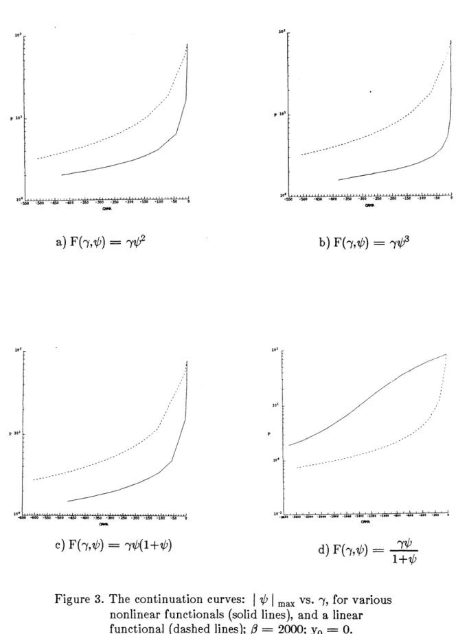
We shall consider (II-1) with various nonlinear functionals. In a search for solutions which resemble large scale circulation, we shall be primarily interested in those which have slow interior flow and are stable. We can-not show streamfunctions of all solutions that were found, but observing the relationship between the 1 | max and the parameter -y is instructive. Figure 3 shows the continuation curves for some nonlinear functionals (solid lines), compared to the curve for the linear one (' = 2000 , yo = 0).

The maximum of the streamfunction decreases with -y, so that for polyno-mial or rational function solution reduces to the linear (this holds for variety of other functionals e.g. -j sinh(@4) , '( eO - 1 ) etc. ). All of these

solutions are stable as long as -1 < 0. For F(@f) = -y e , situation is more complicated. First, we note that these solutions do not satisfy (11-3) (it is violated at 4 = 0), and may be unstable. Nevertheless, since _0max'

decreases with -1, we expect that the pattern for I

>>

to the Fofonoff's gyre. Indeed, single gyre flow with yo = 0, is almost the

same as the linear one, except for appearance of a weak westward boun-dary current at yo. If n is odd, and yo > 0 this current will occur at the latitude yo.

- 20 -S 00 1450 400 -250 -200 - - ' ' a) F(-,k) = 101 . p 101 -600 -550 -500 -450 -400 -350 -300 -250 -200 -150 -100 -50 0 p 10~ -55 -500 -450 -00 -350 -300 -25 -200 -150 -100 -M 0 b) F(-y,/) 3 001 10' -101 .2111 -2200 -1202 -1112 -1222 -1222-1*2*-221 422 -All -Ill c) F(-y,@O) = @b(1+ b) _{d) F(',@)}

-Figure 3. The continuation curves: | @| ma vs. -y, for various nonlinear functionals (solid lines), and a linear

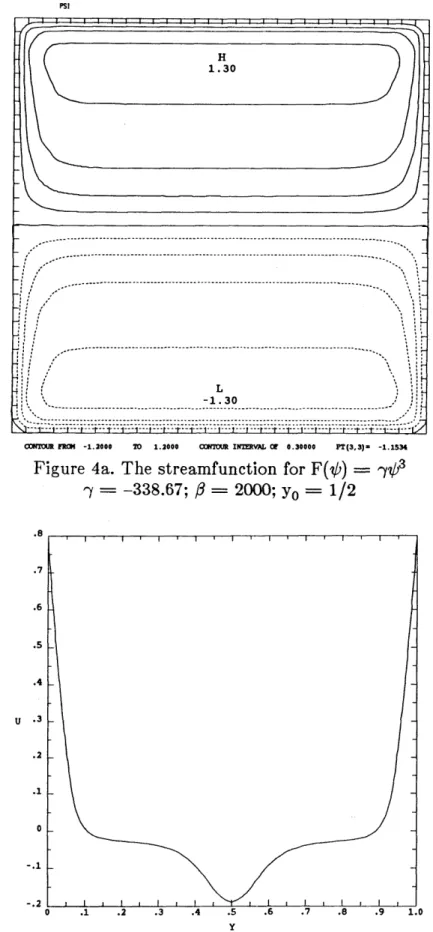
L -1.30

COmrOUR FROM -1.2000 TO 1.2000 CONTUR INEVL OF 0.30000 PT(3,3)= -1.1534

Figure 4a. The streamfunction for F(O) = -y?

- -338.67; # = 2000; yo = 1/2

Figure 4b. Profile of the east-west velocity, u(y), at x=1/2 (m/s) H

- 22

-It is much wider and slower than the boundary currents, but faster than the return flow (Fig. 4). For n even and yo / 0,1, it is clear from parity considerations, that there will be a region in the basin (other than the boundary layer) where F(k) cannot balance the f-term, so that the relative vorticity must be large. This will in general produce a very strong large vortex. In the next example, a similar vortex will appear, but with more interesting properties.

Let

F ( 6 , ,)=6 @ ( 1 + ) (11-4)

Equation (II-1), with (11-4) has two solutions for -y E [ T', 0 ) and y c ( 0,

T" ], where T' and T" are left and right turning points. This will hold pro-vided that 0 < yo < 1, and # is sufficiently large (e.g. for small # say

,8=50 only one solution was found in the interval - 700 < -j < 700). A

typical continuation curve of the dependence of the maximum of the abso-lute value of the streamfunction on -y is shown in Figure 5

()= 2000; 6 = -1.250). The dashed curve is symmetric with respect to the axis -y = 0, since yo = 1/2; as yo -+ 0 the right turning point will shift

to + oo and for yo = 0 only one solution was found in the right half of

the (-y, 0 m| . ) plane (solid curve). Analogously, the shift yo -+ 1

causes T' -+ - oo. To the right of the turning point T, the pattern of the flows is essentially the same as the linear one (Fig. 2). However, due to the nonlinear term, the boundary current may be wider and interior velocity cannot be constant, but slowly varies.

103 102 p 101 100 T - A T' 10~1

[

a) I 0(y) max; T,T',T" are the turning points. V denotes the solution shown in the Figures 7.

F denotes Fofonoff's solution (Fig. 2)

V

I I I I - . -. 8 -. 6 -. 4

I *l''I I i I I i

-. 2 0 .2 .4 .6

b) -y

I

I

#

6 = -2500; yo = 0 (solid curve); yo = 1/2 (dashed curve)

V .6 .4 0 -. 2 -. 4 -. 6 T' -. 8 -1.0 -1.2 -1.4 -1.6 -1.8 -2.0 -2.2 -2.4 L -1.0 T8 T' .8 1.0 1.2 T't

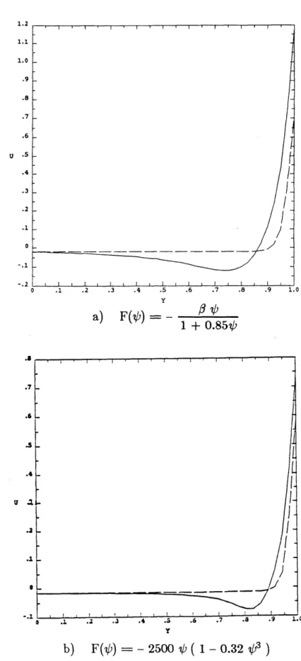
-24-1.2 1.1 1.0 .9 .8 .7 .6 U .5 .4 .3 .2 .1 0 -. 1 -. 2 L L L 0- . .2 .3 .4 .5 .6 .7 .8 .9 1.0 Y a) F( ) -1 + 0.85 .7 .. 8. Y b) F(9) =- 2500 (1 - 0.32iP3 )

Figure 6. Profile of the east-west velocity, u(y), at x = 1/2 for two nonlinear functionals (solid curves), and a linear functional (dashed curves).

Estimates of the width of the inertial boundary layer (Pedlosky

(1979)) are usually given with the assumption that the streamfunction has

small amplitude, i.e. it is effectively reduced to Fofonoff's model. In midla-titudes with 8 = 2000, the interior velocity is U = 2 cm/s and scale length L = _{2000 km, so the dimensional width is 6U} =

(

#o

For nonlinear F, the width may be substantially larger. In Fig. 6 profiles of the east-west velocity at x = 0.5 (1000km) for two nonlinear functionals

(solid curves) are compared with the profile of the linear one (dashed curves). Increase of the eastward transport is compensated by the appear-ance of the counterflow on the seaward side of the boundary current. This phenomenon is observed in nature and is usually described as a conse-quence of friction (see e.g. Pedlosky (1979)). As our result shows, it may well be regarded as a purely inertial effect.

By solving (II-1) with (1-4) for various values of -y, it can be shown

that the condition (11-3) holds for all solutions on the continuation curve to the right of the point A (solid curve), and between points A' and B' (dashed curve in Fig. 5). Solutions with the velocity profiles given in Fig. 6 are also stable.

Above the turning point T (Fig. 5) solution changes character. If 0 is relatively small (e.g. 200), when -Y increases there develops a strong large eddy which covers more than half of the inertial gyre. Such a flow is not relevant for oceanic circulation since the particle speed in the interior is too large.

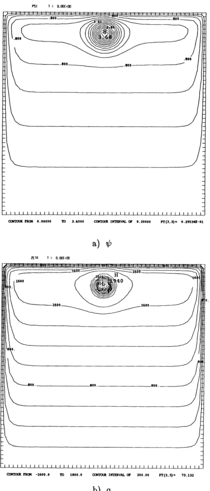
- 26 -PSI T : O.00E4

CXNEUR FRC 0.00000 TO 3.6000 (X)NTOU INTERVAL OF 0.20000 PT(3.3)= 0.29534E-01

ZETA 7 = O.IE400

CXNTOUR FROM -1600.0 TO 1800.0 CONTOUR INTERVAL OF 200.00 PT(3,3)= 73.132

b) q

Figure 7. The streamfunction (a) and the potential vorticity (b) for

0.0 0.0 0.0 .800 _0. - . 0 L -. 087 1 I I I I I I I I I I I I I I I I i I I I i i |

CONTOUR FROM 0.00000 TO 1.0000 CONTOR INTERVAL O 0.10000 PT(3,3)= -0.31431E-01

a) g ZETA2 .180 .10 01. - 0.0 0.0 .0.0 0.0 - 070 0.0. .69-3/0.0 0. 0.0 - ~- . 090

CON70UR FRM 0.00000 10 0.45000 CONTOUR INTERVAL O 0.90000E-01 PT(3,3)= -0.31431E-01

r-r_{0 2}

b) [g - e 0.032

Figure 8. The enlarged area of the vortex [0.40,0.60]x[O.79,0.99] showing normalized vorticity (a) and the vorticity after subtracting the radially symmetric part (b)

- 28

-However, as 8 increases the flow becomes slower, and the eddy becomes smaller eventually ( at 8 = 2000 ) _{degenerating into a vortex of the size of}

mesoscale eddy near the boundary current (Fig. 7). In Figure 5. the point V denotes this solution on the continuation curve.

In the vortex core, the nonlinear term in F (-y, #) is larger than the linear (Fig. 5b) and F has the same sign and nearly the same magnitude as the

#-term.

negli-gible, so that the velocity varies from 1.7 cm/s at the southern boundary to 3 cm/s in the northern part. Boundary current and the vortex have particle velocities of 0.5-0.8 m/s, and contain almost all energy of the flow. The eddy is nearly radially symmetric. Taking for the edge of the vortex point where the streamfunction is a half of its maximum value, we find an east-west diameter of 270 km and a north-south diameter of 240 km. The structure of the flow becomes clearer after subtracting the radially sym-metric part. Let

1 = ( g - exp ( R2_))/imax

where is the relative vorticity of the flow, R = ( r - ro )/a , ro is the center of the vortex and a is small number which depends on properties of the vortex (which in turn are determined by 3 and - ) here a = 0.032. 1 (Fig. 8) contains a weak asymmetric dipole. Its southern (stronger) part

is less than 10% of

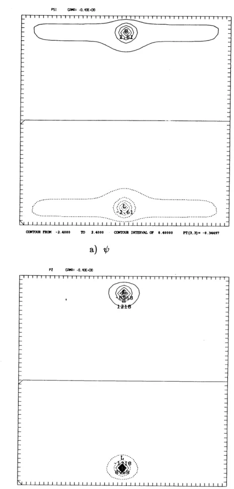
gmax-The above described solution holds for yo = 0. On the other hand, if Yo = 1 and - > 0 one obtains a solution in the form of gyre with the

PSI GANA= -0.40E400

11 i I I I I i Il I I I i I I i i i I I I I T

CONTOU FR -2.4000 TO 2.4000 CONTOUR INTERVAL OF 0.40000 PT(3,3)= -0.34497 a)#

P1 CAM= -0. 4E400

_ i I I I i i i i i I I T- I I I II I I I II I i i i I II

N i l [ 1 i i i 1 1 1 1 1 1 1 1 i1 1 1 1 1 i i i1ii i 1 i i i i _{1 1 1 1 1} i i i i CONTOUR FROM -8000.0 TO 8000.0 CONTOUR INERVAL OF 1000.0 PT(3,3)= -657.23

b) q ,

Figure 9. The streamfunction (a) and the potential vorticity (b) for

- 30

-Note that the vortex has always the same sign of the vorticity as the gyre in which it is embedded.

As in Fofonoff's solution (see e.g. Pedlosky (1979) p. 289), when

0 < yo < 1, the pattern will consist of two gyres, which between the

turn-ing points T' and T" (dashed curve in the Figure 5) is similar to the linear one, except that the northern boundary current is wider if -y < 0 while the southern one remains in the linear regime. The opposite happens when

, > 0. Above the left turning point T', the northern gyre will develop a

small anticyclonic vortex like the single gyre solution, while the southern one will remain unchanged. Similarly, above the right turning point T", the southern gyre will contain a cyclonic vortex.

For higher order correction,

F ( 6 , , V) ) = 6 (1 + ")(1-5)

the solution for yo = 0,1 is similar to that of Fig. 7, except that the vortex

is smaller and more intense. If n is even, F is odd function of 0 and when

YO / 0,1, there will be two vortices near both the northern and southern

boundary current (Fig. 9). We have solved (II-1) with (11-5) for n =2,3,4, but we expect that the same conclusions would hold for higher powers. In contrast with previous solutions describing small vortices which exist only for certain functional and moreover only for certain parameter values (those which satisfy some "dispersion relation"), our solution apparently exists for an entire class of functionals and for parameter values which may change continuously.

In the recent work of Malguzzi and Rizzoli (1984), equation (II-1) was solved in a channel with F as in (11-5) with n=2. They obtained a dipole superimposed on a shearing flow with cubic profile. However, their result is fundamentally different from ours, because their solution exists only if the nonlinear term 'y@/2 is small compared to unity (though not infinitesimal, this is a "weakly nonlinear problem"). Our solution with vor-tices can exist only if the nonlinear term is sufficiently large. More specifically, it exists only above the turning point when 1 -1

#

10b), and for the strong vortex of Fig. 7 | -i 0 | max ~ 1.2, i.e. it

dom-inates the linear term. Figure 5b shows how the product |YO

I

changes with -y for the same data as in the Figure 5a. As -y -+ 0, the

pro-duct reaches the asymptotic value of -2.4. This limit is associated with the second singular point of the partial differential operator in (II-1), the first one being the turning point T. In the next section we shall examine the stability properties of such solutions.

Our procedure does not guarantee that all solutions of equation (11-1) for given F will be found. There may be additional solutions on disjoint branches, which could be found if the number of variable parameters is increased. One such example will be described in the Chapter III in the context of two-layer flow.

For a single layer, we found no physically relevant bifurcation points, although in some cases, e.g. F = -y sin (

4

>>

- 32

-the mesh.

There is no physical reason why, for inertial flows, any one particular relationship between potential vorticity and streamfunction which satisfies the conditions of having a slow interior flow and being stable should be favored over another. We have examined solutions for a number of func-tionals to see how the flow pattern changes. Only funcfunc-tionals such that F(O) = 0 were considered (this is not restrictive because if the first term in

the Taylor expansion of F is a constant it can be absorbed in yo).

For all solutions that we computed, which satisfy the above stated

con-ditions the basic pattern is qualitatively the same as Fofonoff's, only in

2 PERTURBATION EXPERIMENTS

Solutions with vortices do not satisfy the Arnol'd-Blumen condition and may be unstable. It is possible to investigate the stability of such flows numerically by solving the normal mode problem. This approach is cumbersome and if no growing modes are found it would still be incon-clusive. Instead, we shall solve the time dependent problem with the initial condition in the form

= _{+o +}

where go is vorticity of the steady solution, and g, is the perturbation:

i=MU j=MU

a3 cos(7rx+wi) cos(iry+wj)

p go i=MUj=MU (11-6)

I

where a are random numbers from the interval [-1/2,1/2], while

wi and o are random numbers from the interval [0,7r]. P measures

rela-tive size of the vorticity of the perturbation and denotes L2 norm: 11

|

I

(ff

go(x,y) dxdy

00

The barotropic vorticity equation

- + _{+ #}

_-

(11-7)

at

ax 5y

-y ax

B

ax

was solved numerically with free slip boundary conditions

(g =

timestepping scheme was leapfrog and the space discretization scheme was second order centered finite differences with the Arakawa formulation of the Jacobian. The experiments with low frequency perturbations were

- 34

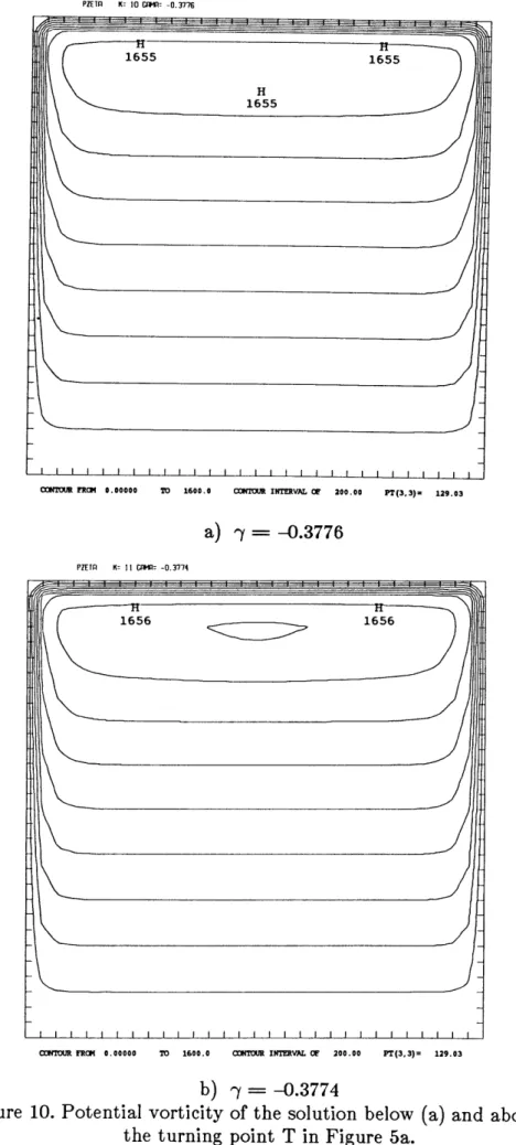
-done on a grid 145x145, and those with high frequency on a grid 257x257. Before we proceed with description of the perturbation experiments we shall examine in which region of the basin the condition (1-3) is violated and how the solution changes in the vicinity of the turning point (Fig. 5). We have examined solutions just to the right, and to the left of the point A (both on the lower branch). Although one of the solutions ("right") satisfies the Arnol'd-Blumen condition and the other does not, there were no qualitative differences. Thus, it is possible that all flows between points A and T are still stable (remember that the Arnol'd-Blumen condition is sufficient, but not necessary for the stability). Near the turning point T, there is a sudden change. Figure 10 shows the poten-tial vorticity of the flow below T (upper plot) and above T (lower plot). Note the appearance of the "hole" in the potential vorticity surface in the place where the vortex will develop. The rest of the pattern is almost unchanged. This suggests that the instability will be confined (at least for sufficiently short time) to the area of the vortex. We plotted potential vor-ticity instead of the streamfunction, because it is much more sensitive to the changes of the parameter -y.

Equation (11-1) with (11-4), was solved with assumption that the Rossby radius is infinite.1

1 The Rossby radius is defined as R = (gD)1/2 where g is gravitational acceleration, D is the depth of the ocean and fo is Coriolis parameter.) For typical parameter values: g = 10ms 2, fo = 104 s 1 and D = 4000 m, we have R = 2000 km, which equals the size of the basin, so the scaled Rossby radius is 1.

PZETP K: 10 CGMPR -0.3776

CONTOUR FRIO 0.00000 TO 1600.0 CONTOUR INTERVAL O 200.00 PT(3,3)= 129.03

a) -y = -0.3776

FIETP 0- It CRM: -0.3774

CONTIOUR FROM 0.00000 TO 1600.0 CONTOUR INTERVAL O 200.00 PT(3,3)= 129.03

b) -y = -0.3774

Figure 10. Potential vorticity of the solution below (a) and above (b) the turning point T in Figure 5a.

- 36

-It is easily seen that our solution (Fig. 7) is also the solution of the vorti-city equation with the effects of surface deformation included:

L 2

(1 -2 ( )2 ) @b + 3 ( y - yo ) + G(-1,6,@ ) 0 (II-8)

where G(Qf,6,i)= 6 @ ( I +

+

<<

6R

_6R2

_i

Recently, Benzi et al. (1982) found that for the barotropic vorticity equation with finite Rossby radius, there are two sufficient conditions for for the stability under small but finite amplitude perturbations: first,

BG

a) 0

<

<

which is a generalization of (11-3), or, second,

b) - oo < < -< ( -)2

8a - L

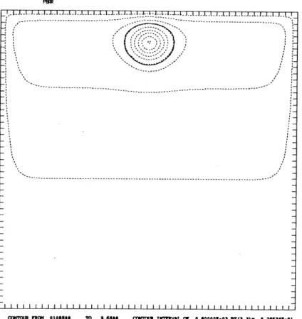
We applied these inequalities to the vortex solution. The basin can be divided into three parts: outside the solid curve (Fig. 11) inequality a) holds, while b) holds within. Actually, these two regions are separated by a gap which is very narrow, because | |

<<

2-6 L2

a) nor b) hold. Both conditions (11-9), as well as (11-3), were derived from integral inequalities and they cannot show how the local instability will occur. Nevertheless, we may expect that the vortex where b) is satisfied, will be robust, and that instability may occur in the annulus that separates it from the surrounding flow.

L-L- J..-.- .-L.L-J-L--- .L-- .J...L.J-J---- - ..-- --- - - --- L- J- .L.--.J. ----J..l.L J. - -- -. .. _

i~ ~~~~~ i i i i i i i i I i I I I I I I I I I I I I I I I I I I I I I I I I I I | I I I I COITOLUR FROM 0108a1 TO 3.689 CONTOUt INTEtRVAL O 0.40000E-03 PT(3,3). 0 .295341-01

Figure 11. Streamfunction of the solution from Fig. 7 (dashed lines). Solid line separates regions satisfying Arnol'd-Blumen condition (outside)

- 38

-To examine the response of the vortex to the perturbations we per-formed a number of perturbation experiments for various magnitudes and frequencies of perturbations. Here we shall show results of three of them.

EXPERIMENT II-1

We shall first consider only low frequency perturbations, i.e. in which the wavelength is of the order the diameter of the vortex or larger. Thus let ML=1 and MU=20 and P = 1 (so the RMS vorticity of the

perturba-tion equals that of the basic flow). Figure 12a shows the streamfuncperturba-tion of the initial condition. The integration time will be relatively short since the characteristic time of the large scale flow is 108_{s or 1157 days, which is}

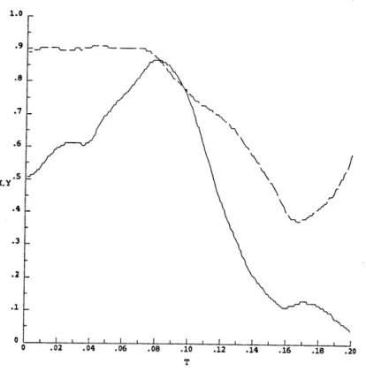
long compared to the characteristic time of the vortex ( O(105s )). Under the influence of perturbations, the vortex moves to the east with nearly uniform velocity ( e 8.5 km/day) and after the time 0.08 (dimensionally

93 days) reaches the boundary. The vortex was not carried by the

boun-dary current since its velocity of translation is much smaller. There is no dispersion prior to the collision (Fig 12b).

There is some ambiguity in determination of the time of collision. One possibility the time when the maximum of the streamfunction of the vortex is closest to the boundary. However, the vortex "feels" the boun-dary earlier, so that it is more appropriate to choose the time when its amplitude starts rapidly decreasing. In this set of experiments another uncertainty is induced by perturbations passing through the vortex, mask-ing the position of its center.

PSI 7=0.000 F= 1 20

.8 29

. i

H -788

.002

CONTOUR FRCa -0.80000 TO 3.2000 CON UR INTERVAL O 0.80000 PT(3,3)= 0.60906E-01

a) Initial condition; ML=1, MU=20, P=1, r=0 O, r=0

PSI T-0.080 F: 1 20

H

RFR -0.00000 TO 4.0000 CONTOUR INTERVAL OF 0.80000 PT(3,3)= 0.12252E-01

b) Streamfunction after t=0.08 (93 days).

-40-.4 _N ' .3 .2 .1 0 I i I i | I L i I 0 .02 .04 .06 .08 .10 .12 .14 .16 .18 .20 T

c) Coordinates of the center of the vortex; x - solid curve; y - dashed curve.

4.4 4.2 4.0 3.8 3.6 3.4 3.2 3.0 2.8 p 2.6 2.4 2.2 2.0 1.8 1.6 1.4 1.2 1.0 .8 .18 .20

d) Magnitude of the streamfunction in the center of the vortex.

Thus, the above estimate of collision time has an error which is less than

D/U, where D is the length of its east-west semiaxis and U is the speed of

translation just before collision (a good estimate being the average speed of translation). Note that the amplitude of the vortex has slightly increased showing that the vortex may gain strength at the expense of the perturbations. After the collision, the vortex moves to the southwest with rapidly decreasing amplitude and after the time 0.20 (232 days) disap-pears. This experiment was repeated with the same ML,MU and P and only the sign of the perturbation changed. As a result the vortex moved to the west with the same speed as in the original experiment.

This experiment was repeated with the perturbations of the same fre-quency and sign, but larger amplitude (P=4). The perturbed vortex moved very rapidly to the east and collided with the boundary after time

0.01 (only 16 days). In this period, there was no decrease of its amplitude

and dispersion was not observed. EXPERIMENT 11-2

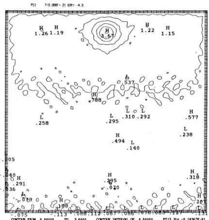
In this experiment we observed the behavior of the vortex under the influence of the high frequency perturbations. Let P = 4, ML = 21, MU = 60 so that the highest frequency perturbation has wavelength less than 1/4 of the vortex diameter. The vortex slowly drifted to the east (Fig. 13ab), and after the time 0.10 (106 days) collided with the boundary. There was no dispersion and the vortex decayed only after the collision (Fig. 13cd).

- 42 -PSI T:0.000F: 21 G0P= -4.0 H .261.19 1.22 H 1.15 0 o 0 L o L H L .310.292 .577 .295 L .258 L .238 H .494 _L .140 -.105 40~ H -40H H .318 .291 4

L. O3.60 C7~0000 aIOOIJ 0INERA

. 36 0 o-040 0 0

, o o H

CONTOUR FROM 0.00000 TO 3.6000 CONTOUR INTERVAL OF 0.60000 PT(3,3)= -0.18367E-01

a) Initial condition; ML=21, MU=60, P=4, r0=0, r=O

PSI T0O.0OFr 21 60P- -4.0

CONTOUR FRCM 0.00000 TO 3.5000 CONTOUR INTERVAL OF 0.70000 PT(3,3)= 0.21736E-01

Streamfunction after t=0.10 (116 days). Figure 13. EXPERIMENT 11-2

-

43-PSI T:O.121r: 21 GOP: -4.0

L if .149.48

~1

1!lII!UIIJlIllHJIIIUIIBII'~UlUlIJllII/l!JllilJlillIIU

CONTOUR FRal -0.50000 TO 3.0000 CONTOUR INTERVALor 0.50000 PT(3.3)= 0.305301!-01

c) Streamfunction after t=O.12 (139 days).

4.0 3.8 3.6 3.4 3.2 3.0 2.8 p 2.6 2.4 2.2 2.0 1.8 1.6 1.4 I I _----L-J 0 .02 .04 .06 .12 .14 .16 .18 .20

d) Magnitude of the streamfunction in the center of the vortex. Figure 13. EXPERIMENT ll-2

-44-EXPERIMENT 11-3

The highest frequency of the perturbations is limited by the resolu-tion of the numerical scheme, so in the previous experiments the smallest wavelength of g, was approximately one third of the diameter of the vor-tex. To reduce the relative wavelength of the perturbation, we consider a vortex from the same class of solutions only with 8 = 200. As we men-tioned in the previous section, in flows with relatively small f, the eddy size will be much larger (this is clear from the scaling: 8 L2). In Figure 14a, we plot the streamfunction (h = - 0.29) of the solution. We shall add perturbations with high frequency (ML=21,MU=40) with RMS vorticity

10 times larger than the RMS vorticity of the basic flow (Fig. 14b). After

the time 0.10 (23 days) the vortex collided with the boundary, but unlike the previous cases, it did not disperse afterwards, but its amplitude increased (Fig. 14cd). This is apparently a consequence of the two-dimensional infrared cascade of energy. In the next Chapter we shall give an example of the large vortex which is destroyed by more energetic high frequency perturbations.

Thus, the steady flow of Figure 5 is unstable under finite amplitude perturbations with the instability manifested by the drift of the vortex. The speed of translation increases with the magnitude of the perturbations and the direction of movement depends only on the nature of perturba-tions. The vortex is very robust and does not disperse until the collision with the boundary or under the influence of very strong perturbations.

I I l i i I Ii 11 1 I I I I iI 111| | | | I I 1| | [1 ONfIDUR FROM 0.00000 TO 5.6000 CONTOUR INTERVAL OF 0.70000 PT(3.3)= 0.16341Z-01

a) The streamfunction: F(#b) = -2504 ( 1 - 0.290 ); yo = 0; 8 = 200. PSI T2U00F: 21 40P=-10.0

T T

I

-

.

I

69

0

(3

0

CONTOUR FRM 0.00000 TO 5.0000 ONTOUR INTERVAL OF 1.0000 PT(3,3)= 0.32775E-01

b) The initial condition; ML=21, MU=40, P=10

Figure 14. EXPERIMENT 11-3

- 46 -PSI T:0. IXF: 1 40P=-10.0 c) 0 after t=0.10 (23 days) PSI T=0. 161F: 21 40P=-10.0 d)

4'

Shearing flow may support a strong vortex ( see e.g. Flierl (1979)). Here, there is weak shear of the basic flow surrounding the vortex. How-ever, since the vortex survives in the perturbed flow with rapidly varying magnitude and direction of velocity, it is unlikely that the shear has an important influence on its motion.

- 48

-3 INFLUENCE OF FRICTION

In the next set of experiments we shall analyze motion of the anticy-clonic vortex induced by the bottom friction without perturbations or forc-ing.

EXPERIMENT 11-4

The steady solution of Fig. 7 was used as an initial condition for the barotropic vorticity equation:

+ J ( ,+ 8y)=- _(II-10)

(9t

The bottom friction coefficient, r, will chosen to be 1 (spindown time equals characteristic time of the large scale flow). Figure 15 shows the evo-lution of the flow. The vortex translates to the west with increasing velo-city and collides with the boundary at the time 0.14 (162 days). The aver-age speed is approximately 5 km/day. Before it is deformed in the collision with the western boundary, the dispersion is extremely small, as can be seen from Fig. 15d (upper curve). Dependence of the distance the vortex travels was found by repeating the first experiment with a larger bottom friction coefficient ( r = 2,3 - spindown time is now 579 and 386 days respectively). From Fig. 15f it is clear that the acceleration of the vortex is proportional to the bottom friction coefficient and increases nearly linearly with time. The distance traveled depends on the time and bottom friction coefficient as:

PSI T 0.12E400

H

.928

B il I 11111111 I I I III If I I 111111111 1111 1111 1 I I II 11111 1 1111111 11 ii111111flII ] I IIiI III H CONTOUR FRC4 0.00000 TO 3.0000 CXIOUIR INTERVAL CE 0.30000 PT(3,3)= 0.46315E-02

a) ip after t=0.12 (139 days); r=1

PSI T I O.1E+00

CONTOUR FRCO 0.00000 TO 1.8000 CONTMUR INTERVAL O 0.20000 PT(3,3)= 0.38117E-02

b) @b after t=0.16 (185 days); r=1 Figure 15. EXPERIMENT II-4

- 50

-PSI T = 0.IE400

00NTUR FR 0.00000 TO 1.6000 CONTUR INTERVAL OF 0.20000 PT(3,3)= 0.41509E-02

c) ?$ after t=0.18 (208 days); r=1 3.8 3.6 3.4 3.2 3.0 2.8 2.6 2.4 2.2 2.0 1.8 1.6 1.4 1.2 1.0 .8

d) Magnitude of the streamfunction in the center of the vortex

upper curve r=1; middle r=2; lower r=3; Dashed curves show the fit (11-12)

1.0 .9 .8 .7 .6 .5 X, Y .4 .3 .2 .1 0 'I,

/

/

ii

/1

~\JI

e) Coordinates of the center of the vortex (x-lower curves; y-upper) solid curves r=1; dashed r=2; dotted r=3

3 .60 .55 .50 .45 .40 .35 .30 PA'D .25 .20 .15 .10 .05 0 /

/

/

/

/

f) Distance traveled by the vortex

lower curve r=1; middle r=2; upper r=3; Dashed curves show the fit (11-11)

Figure 15. EXPERIMENT 11-4 i I i ! . I i 1 i ! ! I ! ! _I

- 52

-where CO is a constant depending on the vortex (i.e. # and -y), but indepen-dent of friction. The dashed curve in Fig. 15f represents the fit (II-11). The vortex translates as a solid body under the influence of the force which is proportional to the bottom friction coefficient. Total energy of the flow slowly decreases. A part of the energy of rotation is, through the influence of bottom friction and the #-effect, converted into the kinetic energy of translation. It is easy to give a crude estimate of the distribution of the spent energy of rotation between dissipation and energy of translation.

By assuming that the vortex behaves as a uniformly rotating cylinder,

its initial energy is entirely contained in rotation: Er(O) = -W

2

where I mR2 - pDR47r is the moment of inertia (D is depth of the

2 2

ocean, R is radius of the vortex and p is density), and w is angular velocity

v

w = R , _{(vr is tangential velocity).}

We shall assume for simplicity that the vortex retains its shape and only its angular velocity decreases with time. Then after the time to, total energy is

E = Er(to) + Et(to) where energy of translation is:

mvt pDR27rv2

2 2

and total kinetic energy at the time to expressed in terms of the initial energy is:

Ek(t) = [ (Vr(t _vr(0) )2 + 2 ( tO)) 2 ] Er(0)

vr(0)

where the first term in the bracket is the remaining energy of rotation and the second is acquired energy of translation. From the slope of the streamfunction in the vortex the tangential velocity can be estimated, ini-tially vr(0) a 80cm/s and after the time to = 0.12, Vr(to) ~ 65cm/s and vt(to) = 10cm/s, then we have:

Er(to) m 0.65 Er(0) Et(to) m 0.03 Er(0)

Thus, of 35% of energy of rotation lost, 32% was dissipated and only 3% was converted to kinetic energy of translation. This "engine" is apparently very inefficient, but may be enough so to make difference in distribution of eddies in the basin. By the assumption that the vortex does not change shape, it follows that the change in angular velocity is proportional to the change of the streamfunction, which changes as ip(0)(1-rt) where r is the bottom friction coefficient. We shall also assume that t<<1 and r is at most 0(1). Since vt is proportional to rt2_{, it follows that the ratio of the}

energy of translation to the dissipated energy after the time t is

Et _ _ _ Cjr2t4 _{C rt}3

Er(0)-Ek(t) 1 - (1-rt)2

where C1 and C are constants and we used the fact that Et(t)

_<<

Thus the efficiency of the "engine" increases with r.

Warren (1967) suggested that the reason for westward movement of the radially symmetric eddies is the #-effect. More recently it was argued

-54

-that the Gulf Stream Rings are advected by the interior flow, although their average speed is larger that of the mean flow (Lai and Richardson

(1977)). In our experiments, /-effect alone cannot account for westward

motion. Indeed, when the vortex was perturbed in the inviscid flow, the direction of motion was dependent only on the nature of the perturbation. This also shows that for our vortex the advection by the mean flow cannot provide a mechanism for the westward movement either. We shall return to the question of westward motion later.

The decrease of the maximum of the streamfunction is slightly faster than linear, which for the time before collision agrees with the fit:

0( xo (t) , yo (t) ) = 0 ( xo (0) , yo (0) ) exp ( - r t) (1-12) where xO and yo are the coordinates of the center of the vortex. From the above relation, it follows that the basic balance in the equation of motion in the region of the largest vorticity is:

atV2 r v2

Fig. 15e shows the x and y coordinates of the center of the vortex. Note

that the southward shift of the vortex increases with the bottom friction. This is usually explained as a consequence of the "form drag instability". This is manifested in the appearance of a countervortex to the south of the main vortex. It cannot be seen in our figures since it is very weak.

In the previous experiment, the bottom friction was turned on abruptly, so it is possible that it just "pushed" the vortex from its (unstable) equilibrium near the boundary current and it later accelerated