HAL Id: hal-00655322
https://hal.archives-ouvertes.fr/hal-00655322
Submitted on 27 Dec 2011
HAL is a multi-disciplinary open access archive for the deposit and dissemination of sci-entific research documents, whether they are pub-lished or not. The documents may come from
L’archive ouverte pluridisciplinaire HAL, est destinée au dépôt et à la diffusion de documents scientifiques de niveau recherche, publiés ou non, émanant des établissements d’enseignement et de
Interval analysis on non-linear monotonic systems as an
efficient tool to optimise fresh food packaging
Sébastien Destercke, Valérie Guillard
To cite this version:
Sébastien Destercke, Valérie Guillard. Interval analysis on non-linear monotonic systems as an efficient tool to optimise fresh food packaging. Computers and Electronics in Agriculture, Elsevier, 2011, 79 (2), pp.116-124. �10.1016/j.compag.2011.08.014�. �hal-00655322�
Interval analysis on non-linear monotonic systems as an
efficient tool to optimise fresh food packaging.
Sebastien Desterckea,b,∗, Valerie Guillardc
aINRA/CIRAD, UMR1208, 2 place P. Viala, F-34060 Montpellier cedex 1, France bLIRMM, UMR 5506, 161 rue Ada, 34095 Montpellier
cUniversit´e Montpellier 2, UMR1208, 2 place P. Viala, F-34060 Montpellier cedex 1, France
Abstract
When few data or information are available, the validity of studies performing un-certainty analysis or robust design optimisation (i.e., parameter optimisation under uncertainty) with a probabilistic approach is questionable. This is particularly true in some agronomical fields, where parameter and variable uncertainties are often quantified by a handful of measurements or by expert opinions. In this paper, we propose a simple alternative approach based on interval analysis, which avoids the pitfalls of a classical probabilistic approach. We propose simple methods to achieve uncertainty propagation, parameter optimisation and sensitivity analysis in cases where the model satisfies some monotonic properties. As a real-world case study, we interest ourselves to the application developed in our laboratory that has motivated the present work, that is the design of sustainable food packag-ing preservpackag-ing fresh fruits and vegetables as long as possible.
Keywords: Interval analysis, robust design, fuzzy sets, sensitivity analysis, uncertainty analysis.
1. Introduction
There are many sources of uncertainties in life science and in agronomy, the main reasons for it being the high variability of living organism and the error of measurement devices. Also, the number of available samples for a given exper-iment may be limited (sometimes even reduced to one sample), due to cost or
∗Corresponding author
Email addresses: [email protected] (Sebastien Destercke), [email protected](Valerie Guillard )
practical limitations. In such situations, it can be hard to determine a meaningful probabilistic model of the parameters, let alone a joint probabilistic model over all parameters. In other situations, uncertainty around a parameter or a constant can be described by expert opinions, and whether these opinions can be faithfully translated by single probabilities is questionable (see, e.g., [28, Sec. 4] or [26]).
In such situations, it may be better to use interval modelling and interval anal-ysis to perform uncertainty studies, simply because determining intervals requires less data and knowledge. Also, using interval analysis amounts to make no as-sumptions about parameter dependencies.
In this paper, we consider dynamical non-linear models describing the evolu-tion of variables, with the aim to optimise some of the parameter values w.r.t. some given objective. In such systems, the values of initial conditions, non-modifiable parameter values or even of the objectives may be ill-known. It is then desirable to perform some uncertainty analysis to achieve robust design. Performing such analysis with classical probabilistic methods [15, 4] usually requires to:
• specify the distribution of each input variable,
• specify the dependency structures between input variables,
• perform (costly) numerical analysis to evaluate the output uncertainty. Meeting such requirements necessitates an important amount of information and data. It also involves the use of techniques having a high computational cost. In practice, when not enough information is available, distribution shapes (e.g., nor-mality) and dependence assumptions (e.g., independence between all variables) are often chosen accordingly to some practical criterion rather than to available information. However, the validity of such choices, not confirmed by experiments or available knowledge, may be questioned, as well as the validity of subsequent analysis results [9]. They then provide overly precise and misleading conclusions, which may in turn lead to unwarranted and non-robust design choices.
When few data are available, an alternative is to use interval analysis [16] to perform the uncertainty analysis, that is to consider that only the bounds in which each parameter may vary are known (an information that is often available). Such an analysis comes down to consider that:
• variable and parameter distributions are unknown (up to their bounds), • dependence structure between variables and parameters is unknown.
Compared to probabilistic analysis, interval analysis can therefore be seen as a conservative analysis, in the sense that it does not make any additional hypoth-esis with regard to the available information, and possibly ignores some of the available information. However, in scientific analysis as well as in robust design, it is safer to use such conservative methods than to make unsupported assump-tions. Also note that, when function f has some monotonic properties [27, 11] (a common case in life sciences and other domains [24, 3], where simple models are often encountered), performing interval analysis may require very few computa-tions compared to, say, probabilistic Monte-Carlo analysis. When these mono-tonic properties are not satisfied, performing interval analysis requires more com-plex techniques [23] with increased computational comcom-plexity (the computational cost then becoming comparable to the one of probabilistic methods). However, whether the monotonic properties are satisfied have no impact on the results con-servativeness of interval analysis.
In this paper, we introduce a set of methods to achieve uncertainty propaga-tion, parameter optimisation and sensitivity analysis on monotonic dynamical sys-tems when uncertainty is described by intervals. Notations and general problem formulations are introduced in Section 2. Section 3 then provides details about the method themselves.
Finally, we illustrate the method on the real-world case study that have mo-tivated the present work and that is currently treated in our laboratory [5] (see website http://www.tailorpack.com/). It concerns the design of sus-tainable fresh food packaging, with the objective to preserve food from decay as long as possible. We use our method to, first, perform uncertainty analysis of a model describing gas exchanges between the packaging atmosphere and exte-rior atmosphere and, second, optimise oxygen and carbon dioxide permeances of packaging materials for a given fruit or vegetable, here chicory. The whole case study is described in Section 4.
2. Problem setting and notations
Vectors of model variables and parameters will be denoted by bold letters (x,p,...), while specific values of these vectors will de denoted by non-bold letters (x, p,...). As the models considered in this paper are multivariate, indexed letters xj will denote the jth element of vector x. Sets will be denoted by calligraphic letters (X ,P,...). The real line will be denoted by R.
We consider a dynamical non-linear model˙x = f (x,pE,pD,t) with f : Rm+n+1→ Rm a time-dependent function that describes the evolution of m state variables
x ∈ Rm, i.e.x = (x1, . . . ,xm). The evolution of these variables depends on nE envi-ronmental parameterspE (whose values cannot be controlled) such as temperature or external pressure and nDdesign parameterspD(which values can be modified) such as mechanical or chemical properties of synthetic compounds. They form a vectorp = (pD,pE) of n parametersp = {p1, . . . ,pn} ∈ Rn.
Given some values p ∈ Rnof the parameters and some initial conditions x(0) ∈ Rm of the state variables, the solution of the system represented by f at time t is x(t) = (x1(t),...,xm(t)) where xi(t) describes the state of the ith state variablexi at time t.
When initial conditions x(0) and environmental parameter values pEare known, a classical design problem [1] consists in identifying the values �pD∈ RnD of the design parameterspD so that the solutions x(t) are as close as possible to a given objective �x(t) on the state variables. However, both the exact values of initial con-ditions x(0), of parameters p or of the objective �x(t) to reach are seldom known with certainty. In the next section, we detail how the problem can be treated when these values become interval and when the model satisfies some monotonic prop-erties.
3. Interval analysis and design optimisation
In this section, we start by giving some refreshers on classical interval analy-sis and interval analyanaly-sis on dynamical monotonic models, illustrating them on a simple example. We then detail our proposed optimisation and sensitivity analysis methods for such models.
3.1. Basics of interval analysis
In the computational literature, interval analysis was first developed to take account of numerical errors [19]. However, interval analysis is now mostly used to perform robustness analysis in applications (robotics [17], chemical, biological, . . . ) where variable values are imprecisely known [16].
A real interval [x] := [x−,x+]of a variable X is a connected and closed subset of R. The set of real intervals is usually denoted IR. An interval vector [x] over Rn(also called box) is the Cartesian product of n intervals. The classical problem of interval analysis consists in replacing, in a given function Y = f (X1, . . . ,Xn) from Rnto Rm, the point valuesx = (x1, . . . ,x
n)of variablesX = {X1, . . . ,Xn} by intervals [x] = ([x1], . . . , [xn])and to compute the range
[x]
f ([x])
[f ]([x])
Figure 1: Illustration of interval analysis with inclusion function (Equation (2)).
Usually, f ([x]) is not a box over Rm, but a complicated subset of it (i.e., it can-not be expressed as a Cartesian product of intervals). Rather than computing the exact propagation f ([x]), one can use guaranteed approximation techniques and compute a box [ f ]([x]) over Rmthat will be an inclusion function, i.e.,
f ([x]) ⊆ [ f ]([x]). (2)
This comes down to compute an outer approximating interval for every dimension of f . The notion is illustrated in Figure 1. Among possible techniques to compute such inclusion functions is interval arithmetics [19], where classical arithmetic operations {+,×,/,−} are replaced by their interval equivalent. Depending on the technique and on the characteristic of the model f , [ f ]([x]) will be more or less close to f ([x]). In the next section, we recall such techniques that can be applied to the particular dynamical models we are interested in.
3.2. Interval analysis to propagate uncertainties in dynamical systems
Let us consider the more complex problem of evaluating the solution of the dynamical system ˙X = f (X,PE,PD,t) with f : Rm→ Rm. In this model, the evo-lution of each state variable Xi, i = 1,...,m is described by an ordinary differential equation (ODE) such that ˙Xi= fi(X,PE,PD,t). The solutions of such systems are m functions xi(t), i = 1,...,m. Here values of function xi(t) are discretised and computed for a finite number of time steps. We denote by T = [0,t] the time domain of the model and assume that each xi(t) is computed for T different times values tk, k = 1,...,T (with tk−tk−1being constant for every k).
For such models, the classical problem of interval analysis is formulated as follows: given m initial conditions xi(0) ∈ [xi](0) := [xi−,xi+](0), i = 1,...,m and n parameters intervals pj∈ [pj], j = 1,...,n, find the bounds [x](t) = [x−,x+](t)
of variable evolutions for each discretised time step t = tk, k = 1,...,T . That is, determine the lower (x−(t)) and upper (x+(t)) envelopes of x(t) for each time step.
Let us call configuration an element of the Cartesian product X := ×mi=1[xi](0)×nj=1 [pj]. Interval analysis on ˙X = f (X,PE,PD,t) then consists in finding, among all configurations in X , those reaching the bounds of x(tk) for each time step tk, k = 1,...,T . As in the non-dynamical case (see Equation (2) and Figure 1), [x](t) can have a very complex shape, hence a slightly easier problem is to find, for each variable Xi, i = 1,...,m, some bounds [xi](t) such that [x](t) ⊆ ×m
i=1[xi](t)
and then to consider the resulting boxes ×mi=1[xi](t) as the solutions. This is the problem we will consider here.
Among the set X of configurations, denote by H = ×n
i=1{xi−,xi+} ×mj=1
{pj−,pj+} the set of extreme ones, that is the set of configurations whose ele-ments are bounds of the intervals. H therefore contains only combinations of such bounds, i.e., 2(n+m) elements, while X contains an infinity of them. To il-lustrate the approach used in this paper, we will use the following simple example: Example 1. Consider the very simple system from R → R
˙
X1= f1(P1) =P1,
where p1∈ [p1] and x1(0) ∈ [x1](0) are positive numbers, and the (analytical) solution of the system is x1(t) = P1· t + x1(0). Here, bothX = X1andP = P1are reduced to a single element each. Our knowledge about p1 and initial condition is given by the intervals p1 ∈ [0.5,1] and x1(0) ∈ [1,3]. The sets of all possible combinations of [p1] and [x1](0), together with their extreme combinations are illustrated in Figure 2. In this example, the set X = [1,3] × [0.5,1], while the set H ={(1,0.5),(1,1),(3,0.5),(3,1)} is reduced to four points.
As for interval analysis on classical functions [11], there exist specific cases [6, 24, 27] where the bounds of [xi](t) on each dimension correspond to solutions of the system ˙X = f (X,PE,PD,t) corresponding to specific points in the set H of extreme configurations, thus reducing the number of necessary computations to find them. Before recalling what are these cases, let us first define the notion of monotonic for dynamical system ˙X = f (X,PE,PD,t).
Definition 1. fi is said to be dynamically increasing w.r.t. variable Xj, j �= i or parameter Pk if
∂ fi
∂Xj ≥ 0 or ∂ fi
X1 P1 1 0.5 3 1
X : All possible couples{p1,x1(0)} H : Extreme configurations
Figure 2: Example 1 set of (extreme) configurations.
and it said to be dynamically decreasing w.r.t. variable Xj, j �= i or parameter Pk if
∂ fi
∂Xj ≤ 0 or ∂ fi
∂Pk ≤ 0 (4)
For a given function fi(or, equivalently, for a given variable Xi), let us denote by P�,i,X�,i and P�,i,X�,i the set of parameters for which fi is dynamically increasing and decreasing, respectively. Note that they are disjoint, i.e. P�,i∩ P�,i= /0 andX�,i∩ X�,i= /0. We also assume from now on that these sets form partitions of the parameters and variables, that is for a given i,P�,i∪P�,i=P and X�,i∪ X�,i=X. When a function fi is dynamically increasing or decreasing in each variable and parameter, the following proposition [24] tells us how the upper and lower envelope of [xi](t) at any time step t can be obtained.
Proposition 1. For any t, the bounds of [xi](t) can be computed as follows: • x+i (t) is the solution of the system ˙X = f (X,PE,PD,t) with the configuration
H i∈ H such that Hi=
P = p+ for all P ∈ P�,i
P = p− for all P ∈ P�,i
X(0) = x+(0) for all X ∈ X�,i X(0) = x−(0) for all X ∈ X�,i
(5)
• x−i (t) is the solution of the system ˙X = f (X,PE,PD,t) with the configuration H i∈ H such that Hi=
P = p+ for all P ∈ P�,i
P = p− for all P ∈ P�,i
X(0) = x+(0) for all X ∈ X�,i X(0) = x−(0) for all X ∈ X�,i
x t 2 4 6 8 10 12 14 1 2 3 4 5 6 7 8 9 10 x− 1(t) : p1=0.5,x1(0) = 1 x+ 1(t) : p1=1,x1(0) = 3
Figure 3: Interval analysis with Example 2 model
This means that if the monotonic properties of fi are known, then one can solve the system with configuration Hi to get x+
i (t), and with H ito get x−i (t). This means that to retrieve the bounds of [xi](t) for any variable Xi, i = 1,...,m, the system ˙X = f (X,PE,PD,t) has to be solved twice with usual techniques not involving intervals. For such systems, propagating uncertainties modelled by in-tervals then becomes much easier than propagating probabilistic uncertainties (it comes down to solve at most 2·m different systems). Let us continue our example. Example 2. Consider the system of Example 1. We have (assuming a positive
P1) that ∂ f1
∂P1 ≥ 0, hence f1 is dynamically increasing w.r.t. P1 and X1. Hence
P�,i =P1, P�,i= /0, X�,i=X1 andX�,i= /0. Hence the upper envelope x+
1(t)
is given by the configuration H1={p+1,x+(0)}, and the lower one by x−1(t) by H1={p−1,x−(0)}. Figure 3 represents the two envelopes when [p1] = [0.5,1] and [x1](0) = [1,3] for t ∈ [0,10].
3.3. Parameters optimisation
We now consider the problem of searching optimal values �pD of design pa-rametersPD when initial conditions and environmental parameters are valued, and when objectives (constraints) �x(t) on the state variables are interval-valued as well. We consider that, for each variable Xi, the objectives �xi: �T → IR can be given over some subset �T ⊆ T of the whole time domain (for instance, constraints on values may only be specified for the steady state only, that is after a time t∗such that �T = [t∗,t], . . . ). Note that objectives can be intervals, as their exact values can themselves be uncertainly known (or there may be many values
that appear as optimal in the context). This way of formulating an optimisation problem is not usual, even in interval-analysis literature [22], where the objective function is usually precisely valued (e.g., corresponds to precise outputs). Again, such a problem may be in general difficult to solve. We propose a general way of formulating the problem, before proposing an easy-to-apply algorithm in the case of monotonic systems (i.e., systems satisfying Definition 1).
Consider some pre-defined objectives [�xi](t) as well as some initial conditions [xi](0), i = 1,...,m and some interval-valued uncertainty [p] for every environ-mental parameter P ∈ PE. Consider some (precise) value �pDfor design parameters PD. Design parameter values �pDare said to form a guaranteed (resp. possible) so-lution if the soso-lution of the system ˙X = f (X,PE,PD,t) with these values �pD(and with given intervals onPE and X initial conditions) is such that [xi](t) ⊆ [�xi](t) (resp. [xi](t) ∩ [�xi](t) �= /0) for every t ∈ �T . We denote the set of guaranteed so-lutions by GD and the set of possible solutions by SD. Both these sets may be empty, but we have the inclusion relationship GD⊆ SD. A guaranteed solution is such that, despite of interval uncertainties, we are certain that with the given design parameter values, the true answer lies within the objective bounds, while a possible solution is such that, with the given design parameter values, the true answer may or may not lie within the objective bounds. Solutions that are totally outside the objective bounds are said non-admissible.
Example 3. Consider again the model of Example 2, except that this time param-eter P1is considered as a design parameter that can be tuned through some control process (e.g., a speed of reaction controlled by some catalyser). Objective �x1(t) on the variable X1 is specified for �T = {10} and is such that [�x1](10) = [8,11]. Fig-ure 4 illustrates the notions of guaranteed, possible and non-admissible solutions for this case. For example, when P1=0.75, we have [x1](10) = [x1−,x1+](10) = [8.5,10.5] and [x1](10) ⊆ [�x1](10).
The exact bounds of sets GD and SD are, in practice, hard to find. However one may search, for each P ∈ PD, intervals [GP] = [gP−,gP+]and [SP] = [sP−,sP+] approximating GDand SD on each design dimension. Those values are the solu-tions of the following optimisation problems (provided such solusolu-tions exist):
gP−=minP, gP+ =maxP, under the constraints
xi(0) ∈ [xi](0), i ∈ {1,...,m}, pj∈ [pj] ∀Pj∈ PE ∀t ∈ �T , i∈ {1,...,m}, x+i (t) ≤ �xi(t)+and x−i (t) ≥ �xi(t)−,
X1 t �x(t) 2 6 10 14 0 2 4 6 8 10 x− 1(t) x+ 1(t) P1=0.75
Fig 4.A guaranteed solution
x t �x(t) 2 6 10 14 0 2 4 6 8 10 x− 1(t) x+ 1(t) P1=0.9
Fig 4.B possible solution x t �x(t) 2 6 10 14 0 2 4 6 8 10 x− 1(t) x+ 1(t) P1=1.1
Fig 4.C non-admissible solution
Figure 4: Illustration of solutions with Example 2 model
and
sP−=minP, sP+ =maxP, under the constraints
xi(0) ∈ [xi](0), i ∈ {1,...,m}, pj∈ [pj] ∀Pj∈ PE ∀t ∈ �T , i∈ {1,...,m}, x−i (t) ≤ �xi(t)+ or x+i (t) ≥ �xi(t)−.
Again, solving exactly such problems is in general difficult. However, when the model1 ˙X = f(X,PE,pD,t) is dynamically monotonic (either increasing or de-creasing) in each variable and each environmental parameter, we propose a simple heuristic method to identify [GP]and [SP]. Algorithm 1 suggests some means to find them when each component of ˙X = f (X,PE,pD,t) is dynamically monotonic w.r.t. a given design parameter P. In this algorithm, HiPE,X and HiPE,X are the configurations of Proposition 1 reduced to environmental parameters and initial conditions, the values of design parameters being left unspecified.
The algorithm simply uses the known monotonic properties of the model to compute boundary values. For instance, consider Lines 2-3 and the case P ∈
Algorithm 1: Approximations of [GP]and [SP]of a design parameter P Input: model ˙X = f (X,PE,pD,t), objectives �xi(t)+ and �xi(t)− on �T , Initial conditions [xi](0) for i = 1,...,m and [p] for all P ∈ PE,
Algid: identification algorithm returning design paramter values Output: Intervals [GP]and [SP]
1 for i = 1,...,m do
2 Run Algid on �xi(t)+ with configuration HiPE,X, get optimal value �p of
P;
3 If P ∈ P�,i, set gP, j+=p, else set gP, j−� = �p;
4 Run Algid on �xi(t)− with configuration HiPE,X, get optimal value �p of
P;
5 If P ∈ P�,i, set gP, j−=p, else set gP, j� += �p;
6 Run Algid on �xi(t)+ with configuration HiPE,X, get optimal value �p of
P;
7 If P ∈ P�,i, set sP, j+=p, else set sP, j−� = �p;
8 Run Algid on �xi(t)− with configuration HiPE,X, get optimal value �p of
P;
9 If P ∈ P�,i, set sP, j−=p, else set sP, j� += �p;
10 GP= [maxj=1,...,mgP, j−,minj=1,...,mgP, j+]with GP= /0 if
maxj=1,...,mgP, j−≥ minj=1,...,mgP, j+ ;
11 SP= [maxj=1,...,msP, j−,minj=1,...,msP, j+]with SP= /0 if
P�,i, then considering the configuration of environmental parameters and initial conditions giving x+
i (t) is the most constraining configuration we can have w.r.t. the objective upper bound �xi(t)+ and such that there is still a chance that �p is a guaranteed solution. We still have [SP]⊆ [GP]. Note that Algorithm 1 works only when f satisfies Definition 1. In more complex cases, approximating sets GD and SD can be done by sampling different values of design parameters and then performing interval analysis (with propagation methods adapted to more general models [23]) to check whether the sampled values are (guaranteed or possible) solutions.
Example 4. Consider again the model of Example 2, with the constraints of Ex-ample 3. Running Algorithm 1 to identify [GP1] and [SP1] gives the following solutions (note that here, initial conditions and objectives [�x1](10) provides each time two points, hence totally determining P1in the equation x1(t) = P1·t +x1(0)): • Line 2 of Alg. 1, i=1: Identification with �x+1(10) = 11 and HiPE,X={x1(0) =
3}, giving �p= 0.8 as solution and gP1,1+=0.8 (since P1∈ P�,1).
• Line 4 of Alg. 1, i=1: Identification with �x−1(10) = 8 and H iPE,X={x1(0) =
1}, giving �p= 0.7 as solution and gP1,1−=0.7
• Line 6 of Alg. 1, i=1: Identification with �x+1(10) = 11 and HiPE,X={x1(0) =
1}, giving �p= 1 as solution and sP1,1+=1
• Line 8 of Alg. 1, i=1: Identification with �x−1(10) = 8 and H i
PE,X={x1(0) =
3}, giving �p= 0.5 as solution and sp1,1−=0.5
Finally (Lines 10 and 11 of Alg. 1), we obtain intervals [GP1] = [0.7,0.8] and [SP1] = [0.5,1] providing approximate values of P1that give guaranteed and
pos-sible solutions, respectively.
The obtained sets [SP]and [GP]for each design parameter P ∈ PDcan then be transformed into fuzzy sets [29]. Indeed, while guaranteed solutions all provide the same satisfaction to the designer or the decision maker (they all ensure that the true solution is within the objective boundaries), possible solutions can be seen as having gradual satisfaction degrees, as some of them will have a more significant overlap with the objective bounds than others.
First recall that a fuzzy setµ : V → [0,1] is a mapping from a space V (here the real line) to the unit interval, whereµ(v) is the membership degree of element
0 0.2 0.4 0.6 0.8 1.0 1.2 1
µ˜p1
Figure 5: Fuzzy set of Example 4
v. A trapezoidal fuzzy number µ˜a : [a1,a4]→ [0,1] is defined by a tuple ˜a =
{a1,a2,a3,a4} of four numbers and is such that
µ˜a(x) = x−a1 a2−a1 if a1≤ x ≤ a2 1 if a2≤ x ≤ a3 x−a4 a3−a4 if a3≤ x ≤ a4 (7) In our case, the fuzzy set degree expresses some satisfaction degree [8] pro-vided by a parameter value w.r.t. an interval-valued objective. We propose, for a design parameter P, to build the trapezoidal fuzzy number µ˜P such that ˜P = {sP−,gP−,gP+,sP+} if Gpi�= /0 and such that ˜P = {sP−,(sP−+sP
+)
/2,(sP−+sP+)/2,sP+}
otherwise. Figure 4 illustrates the fuzzy number obtained in Example 4. 3.4. Sensitivity analysis
When performing an uncertainty analysis, it is usual to perform it along with a sensitivity analysis [13, 25, 14]. Sensitivity analysis consists in searching what input parameters or variables most contribute to the output uncertainty. Its results indicate the parameter or variable on which experimental efforts should concen-trate in order to reduce the output uncertainty. Note that there are only very few works dealing with sensitivity analysis of interval approaches [18], contrarily to probabilistic approaches.
In this paper, we propose a very simple method to perform this sensitivity anal-ysis for a given function fi. Let [xi](t) be the interval-valued output resulting from initial interval uncertainty. Then, if we denote by L(xi(tj)):= (x(itj) +−x−i (tj))
the length of [xi](tj) for any time-step tj, we can define the overall imprecision I(xi(t)) of xi(t) as I(xi(t)) := T
∑
j=1 L(xi(tj)), (8)that is, the sum of interval lengths obtained at each time step. Now, to quantify the impact of each parameter and variable uncertainty on the output imprecision, we propose the following procedure (similar to some existing propositions in im-precise probability literature [10]): reduce, for each parameter and variable, its uncertainty by a given fraction r ∈ [0,1], such a reduction coming down to trans-form an interval [a,b] into an interval [a�,b�]such that
a�=M([a,b]) −�L([a,b]) 2 (1 − r)
�
, b�=M([a,b]) +�L([a,b])2 (1 − r)�, (9) with M([a,b]), L([a,b]) the middle and length of the interval, respectively.
Such a reduction gives a new interval-valued solution [x�
i](t) included in the previous one, and with an overall imprecision I(x�
i(t)) ≤ I(xi(t)). If [x�i](t) is the output obtained after reducing the imprecision of parameter P (or variable X) by r, the gain in the output precision generated by this reduction can then be defined as
G(P,r) := (I(xi(t)) − I(x�i(t))
I(xi(t)) . (10)
Let us illustrate this notion in our example.
Example 5. Let us consider again the model of Example 1, with initial uncer-tainty given by p1∈ [0.5,1] and x1(0) ∈ [1,3], the resulting x1(t) being pictured in Figure 3. We have I(xi(t)) = 70 (in this case, the area between the two lines of Figure 3 can be computed analytically).
If we reduce the uncertainty of P1 and X1(0) by 50 % (r = 0.5), we get p�1∈ [0.625,0.875] and x�
1(0) ∈ [1.5,2.5]. We then have
G(P1,0.5) =70−45/70� 0.36, G(X1,0.5) =70−60/70� 0.14.
From these results, it appears that reducing the uncertainty of P1 by 50 % has a more important impact on the output than reducing X1(0) uncertainty by the same amount. Hence, further experiments should focus on reducing the uncertainty around P1.
Finally, note that a reduction of 100 % (r = 1) of a parameter or variable comes down to consider the middle point of the interval it belongs to.
4. Application to food packaging
In this section, we apply the above framework to the design and optimisation of food packaging material, with the aim to maximise shelf life of packaged food (here, fresh fruits and vegetables). Note that this model will be integrated to an online decision support system (http://www.tailorpack.com/), hence quick computations and approximate (but reliable) answers should be privileged over more exact but computationally more demanding answers.
4.1. Problem presentation and model analysis
Preserving fresh food after harvest and on the shop shelves is an important issue in the food industry. Providing food with optimised packaging is a sure way to avoid premature decay and prolong food edibility. Such optimisation means that the packaging must be permeable enough to oxygen and carbon dioxide so as to allow food respiration, but not too permeable to these two gases, so that maturation and decaying process are slowed down.
In modified atmosphere packaging, oxygen and carbon dioxide partial pres-sures in packaging head-space are modified and settle to steady values after a transient phase. This modification in the internal gas partial pressures is achieved due to the mass balance between oxygen and carbon dioxide flux through the packaging material and O2 and CO2 consumption/production due to the product respiration. For a given fruit or vegetable, it is possible to experimentally deter-mine (up to some uncertainties) oxygen and carbon dioxide partial pressures that will result in an optimal preservation. From these optimal partial pressure values, it is then possible to determine optimal packaging permeances, by using a mathe-matical model predicting the dynamic evolution of internal gases partial pressures. Several environmental parameters must be specified in this model such as respi-ration rate or respiratory quotient, packaging geometry, or environment variables such as temperature. The mass balance between gas transfer and respiration can be written as: ˙ pOpkg2 = PeO2· S e (pextO2− p pkg O2 )− RRO2· m = f1 (11) ˙ pCOpkg2= PeCO2· S e (pCOext2− p pkg CO2) +RRO2· m · QR = f2 (12)
Parameter Name Units
PeO2 O2permeance mol.m−1.s−1.Pa−1
PeCO2 CO2permeance mol.m−1.s−1.Pa−1
S pack. surface m2
e pack. thickness m
pi
j partial press. of j in i %
RRO2 O2respiratory rate mmol.kg−1.h−1
RRO2max max. O2respiratory rate mmol.kg−1.h−1
KmappO2 Micha¨elis-Menten constant kPa
KiCO2 CO2inhibition constant kPa
m food mass kg
QR respiration coefficient ×
Table 1: Parameters names and units. ×= non-relevant.
with RRO2 = RRO2max· p pkg O2 (KmappO2+pOpkg2 )· � 1 + p pkg CO2 KiCO2 � (13)
where the first part of the right-hand side describes gas flux per time unit through the packaging material, while the second part describes gas consumption (and emission) by the vegetable or fruit (modelled using a Micha¨elis-Menten-type equa-tion, see (13)). There are two variablesX = {pOpkg2 ,pCOpkg2}. Table 1 summarises the parameters with their names and units, while Table 2 summarises whether they are variable, environmental or design parameters, and their monotonic w.r.t. each function f1and f2. Note that (pextO2− pOpkg2 )is always positive, while (pCOext2− p
pkg
CO2)
is always negative, that pext
i are constant and that all parameters are positive (oth-erwise model would not be monotonic w.r.t. every parameter).
4.2. Case study: chicory
Note that in our case study, the shape of the packaging (S and e) and the mass (m) of food inside it have already been fixed, so that the only parameters that can be adjusted to optimise the packaging are the material permeability properties (PeO2 and PeCO2). Note that, if a probabilistic approach was used, no less than 9 probability distributions would have to be specified, and independence between variables would have to be assumed, with some of the parameters sometimes mea-sured only 3 times. Also, estimating boundaries by interval analysis for pOpkg2 and
Parameter PD,PE,X f1 f2 PeO2 ∈ PD P�,1 × PeCO2 ∈ PD × P�,2 S ∈ PE P�,1 P�,2 e ∈ PE P�,1 P�,2 pij ∈ X X�,1 X�,2 RRO2 ∈ PE P�,1 P�,2 RRO2max ∈ PE P�,1 P�,2 KmappO2 ∈ PE P�,1 P�,2 KiCO2 ∈ PE P�,1 P�,2 m ∈ PE P�,1 P�,2 QR ∈ PE × P�,2
Table 2: Parameters type and monotonic w.r.t. f1,f2. ×= non-relevant.
pCOpkg2 here requires only 4 simulations (far less than for a Monte-Carlo simula-tion [13]).
The considered food is chicory, which has been previously studied, but without any proper uncertainty analysis [5].
4.2.1. Uncertainty propagation step
Knowing the permeability of the packaging material classically used to pack chicory, the mathematical model described by Eq (11)-(13) can be used to simu-late the evolution with time of the internal O2 and CO2 partial pressures. Parame-ters with their interval uncertainty are summarised in Table 3. Maximal shelf life is estimated to be 200 hours, therefore the simulation time domain is T = [0,200]h and the domain is discretised so that each time step is one minute.
The results of interval analysis are displayed in Figure 6, and we can see that, at the steady states, pOpkg2 ∈ [1.6,8.1]% and pCOpkg2 ∈ [1.9,5.3]%. Using
Propo-sition 1, only four simulations were needed (two for each gas) to estimate the bounds.
Also note that, in the current case, initial conditions pOpkg2 (0) and pCOpkg2(0) for the two variables are perfectly known and only parameters are uncertain, as initial partial pressures are the same as in free atmosphere (21% for oxygen and 0% for carbon dioxide). Therefore, only uncertainty pertaining to environmental and design parameters PE and PD have to be taken into account here (contrary to Example 1, where x1(0) value is also uncertain).
Parameter Uncertainty Unit PeO2 [878,1278]10−18 mol.m−1.s−1.Pa−1 PeCO2 [3614,4634]10−18 mol.m−1.s−1.Pa−1 S [12,16]10−2 m2 e [4,6]10−5 m m [0.45,0.55] kg RRO2max [1.3,1.5] mmol.kg−1.h−1 KmappO2 [8.26,10.26]103 kPa KiCO2 [1025,2025]103 kPa QR [0.67,0.81]
Table 3: Parameters uncertainty for propagation.
0 20 40 60 80 100 120 140 160 180 200 0 2 4 6 8 10 12 14 16 18 20 Time (hours)
Gaz partial pressure (%)
!"#$%&'()(*+$#&$%,",$-*,-*./*0-1*2./*!*2./*2.345676785*79:7;767.9 O2Max O2Min CO2Max CO2Min
! !"# $ $"# % %"# & &"# '(!)!!# ) )"$ )"& )"* )"+ ! !"#$%&'(")*%)&+,)-(.+/)*(.+,)*#&$+#0(!(!1 ,-./-012-(3/45"/!!"6!!",0!!7
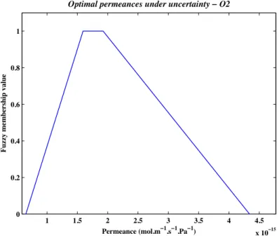
89::;(/-/<-.6=>?(@059-Figure 7: Optimal O2 permeance
!"# !"$ !"% !"& ' '"# '"$ '"% '"& # ()'!!'$ ! !"# !"$ !"% !"& ' !"#$%&'(")*%)&+,)-(.+/)*(.+,)*#&$+#0(!(1!2 *+,-+./0+)1-23"-!'"4!'"*.!'5 67889)-+-:+,4;<=)>.37+
4.2.2. Optimisation step
In the case where best oxygen and carbon dioxide permeabilities suiting a particular fruit or vegetable are not known a priori, it is possible to use Equa-tions (11)-(13) to perform a reverse engineering task. In this case, optimal oxygen and carbon dioxide concentrations in the packaging modified atmosphere have to be specified. Once this is done, Algorithm 1 can be run to find optimal permeabil-ities that allow reaching the specified goal.
In this study, Algorithm 1 was run with the same uncertainty on environmen-tal parameters as the one of Table 3 (i.e., all parameters except packaging mate-rial permeabilities to O2 and CO2, which are the design parameters). Given that T = [0, 200]h and the fact that there exists a transient phase, we have chosen
�
T = [150, 200], �pOpkg2 (t) = [4,10]% and �pCOpkg2(t) = [2,5]% for every t ∈ �T , that is we want oxygen partial pressure to be between 4 and 10 % and carbon dioxide partial pressure to be between 2 and 5 % at the steady state. Fuzzy sets obtained from Algorithm 1 and from the intervals [GPeO2] = [1.59,1.92]10−15, [GPe
CO2] =
[4.94,7.50]10−15 and [SPe
O2] = [4.34,6.51]10−15, [SPeCO2] = [1.78,19.96]10−15
(values are expressed in mol.m−1.s−1.Pa−1) are shown in Figures 7 and 8 (Levenberg-Marquardt Algorithm [21] was used to identify parameters). Figure 9 shows the result of the interval analysis done with optimal parameters belonging to [GPeO2]× [GPeCO2]. We see that the resulting imprecise oxygen and carbon dioxide partial pressures well lie in the objective bounds at the steady state.
4.2.3. sensitivity analysis
Table 4 summarises the sensitivity analysis performed according to the method presented in Section 3.4. For each variable pOpkg2 (t) and pCOpkg2(t), we have evaluated the precision gain after an uncertainty reduction of r = 0.5 of each (environmental and design) parameter. The last column (All) indicates the gain in the output precision when all parameters uncertainty is reduced by r = 0.5.
The results indicate, among other things, that while O2 permeability uncer-tainty has an important impact on both O2and CO2internal partial pressures un-certainty (the reduction resulting in a gain of about 0.1 for each), CO2permeability uncertainty only impact the CO2 internal pressures, and have almost none effects on O2internal pressure. As could be expected, the respiration rate QR uncertainty only impact on the CO2 internal pressure, while KiCO2 uncertainty, due to the large value of KiCO2, has (almost) no impact on the resulting uncertainty for both variables.
0 20 40 60 80 100 120 140 160 180 200 0 2 4 6 8 10 12 14 16 18 20 Time (hours)
Gaz partial pressures (%)
!"#$%&'()(*+$#&$%,",$-*,-*./*0-1*2./*!*2./*2.345676785*79:7;767.9 ! ! Simulation parameters !"#!$%&'%()*%+!,-./0/%!1,/ !2"#!$%&'%()*%+!3-###,%!1,/ O2Max O2Min CO2Max CO2Min O2MaxObj O2MinObj CO2MaxObj CO2MinObj
Figure 9: Uncertainty propagation with optimal permeances
P PeO2 PeCO2 e S m
pOpkg2 (t) 0.099 0 0.124 0.077 0.088
pCOpkg2(t) 0.095 0.12 0.077 0.058 0.024
P QR RRO2max KmappO2 KiCO2 All
pOpkg2 (t) 0 0.057 0.045 0 0.501
pCOpkg2(t) 0.094 0.02 0.019 0 0.505
Table 4: Values G(P,0.5) of sensitivity analysis on the parameters P after a reduction r = 0.5, for the two variables pOpkg2 (t) and pCOpkg2(t)
partial pressures, one should focus on a better characterisation of O2permeability and thickness, and on O2/CO2permeability, respectively.
5. Conclusion
Interval analysis is a useful alternative to probabilistic analysis that requires far less information to be applicable, thus avoiding the need to introduce hypothesis unsupported by available information. In some situations where the models satisfy some monotonic properties, using intervals is also more computationally efficient, as sampling methods are not needed to achieve computations. In this paper, we have used interval analysis for two purposes: classical uncertainty propagation for monotonic dynamical models and robust design under uncertainties. We have also proposed an easy method to perform some first sensitivity analysis.
The proposed robust design optimisation method, although approximate, quickly produces optimal values for design parameters. It takes account of interval un-certainty and can cope with imprecisely specified goals, distinguishing between possible solutions (potentially satisfying the goal) and guaranteed solutions (cer-tainly satisfying the goal). The difference between the two kinds of solutions is represented by the means of fuzzy sets describing optimal solutions.
Methodological perspectives to this work include the development of more precise methods, eventually ending up with better and multi-dimensional approx-imations of the sets GD and SD. Also, it may be desirable to extend the current approach to hybrid uncertainty models mixing interval and probabilistic uncer-tainty [3, 2, 12, 20], as information concerning different parameters may vary in quantity and quality. However, these two perspectives would involve more compu-tationally demanding procedures, thus reducing the number of models one could work with.
More applied perspectives include the combination of the optimisation system with a decision support system where a user can search a database for optimal packaging [7] (fuzzy sets describing sets of optimal solutions will then be used as user preferences) and the application of the system to other food products (such as mushrooms).
References
[1] Aster, R. C., Borchers, B., Thurber, C. H., 2005. Parameter Estimation and Inverse Problems. Academic Press.
[2] Baudrit, C., Guyonnet, D., Dubois, D., 2006. Joint propagation and exploita-tion of probabilistic and possibilistic informaexploita-tion in risk assessment. IEEE Trans. Fuzzy Systems 14, 593–608.
[3] Baudrit, C., H´elias, A., Perrot, N., 2009. Joint treatment of imprecision and variability in food engineering: Application to cheese mass loss during ripening. Journal of Food Engineering 93 (3), 284–292.
[4] Bedford, T., Cooke, R., 2001. Probabilistic Risk Analysis. Foundations and Methods. Cambridge University Press, UK.
[5] Charles, F., Sanchez, J., Gontard, N., 2005. Modeling of active modified at-mosphere packaging of endives exposed to several postharvest temperatures. Journal of Food Science 70, 443–449.
[6] Delanoue, N., 2009. A new method for integrating ode based on monotonic-ity. In: SWIM 09, A small workshop on Interval Methods.
[7] Destercke, S., Buche, P., Guillard, V., 2011. A flexible bipolar querying ap-proach with imprecise data and guaranteed results. Fuzzy Sets and Systems 169 (1), 51–64.
[8] Dubois, D., Prade, H., 1997. The three semantics of fuzzy sets. Fuzzy Sets Syst. 90 (2), 141–150.
[9] Ferson, S., Ginzburg, L. R., 1996. Different methods are needed to prop-agate ignorance and variability. Reliability Engineering and System Safety 54, 133–144.
[10] Ferson, S., Tucker, W. T., 2006. Sensitivity analysis using probability bound-ing. Reliability Engineering and System Safety 91, 1435–1442.
[11] Fortin, J., Dubois, D., Fargier, H., 2008. Gradual numbers and their appli-cation to fuzzy interval analysis. IEEE Transactions on Fuzzy Systems 16, 388–402.
[12] Fuchs, M., Neumaier, A., 2009. Potential based clouds in robust design op-timization. Journal of statistical theory and practice 3 (225-238).
[13] Helton, J. C., Johnson, J. D., Oberkampf, W. L., Sallaberry, C. J., 2006. Sensitivity analysis in conjunction with evidence theory representations of
epistemic uncertainty. Reliability Engineering and System Safety 91, 1414– 1434.
[14] Helton, J. C., Johnson, J. D., Sallaberry, C. J., Storlie, C. B., 2006. Survey of sampling-based methods for uncertainty and sensitivity analysis. Reliability Engineering System Safety 91 (10-11), 1175–1209.
[15] Hertog, M. L., Lammertyn, J., Scheerlinck, N., Nicolki, B. M., 2007. The impact of biological variation on postharvest behaviour: The case of dy-namic temperature conditions. Postharvest Biology and Technology 43 (2), 183 – 192.
[16] Jaulin, L., Kieffer, M., Didrit, O., Walter, E., 2001. Applied Interval Analy-sis. London.
[17] Jaulin, L., Kieffer, M., Walter, E., Meizel, D., 2002. Guaranteed robust non-linear estimation with application to robot localization. IEEE Trans. on Syst., Man and Cybern. C 32 (4), 374–381.
[18] Moens, D., Vandepitte, D., 2007. Interval sensitivity theory and its applica-tion to frequency response envelope analysis of uncertain structures. Com-puter Methods in Applied Mechanics and Engineering 196 (21-24), 2486 – 2496.
[19] Moore, R., 1979. Methods and applications of Interval Analysis. SIAM Studies in Applied Mathematics. SIAM, Philadelphia.
[20] Nassreddine, G., Abdallah, F., Denoeux, T., 2010. State estimation using interval analysis and belief-function theory: Application to dynamic vehicle localization. IEEE Trans. on Syst., Man and Cybern. B 40, 1205–1218. [21] Nocedal, J., Wright, S., 1999. Numerical Optimization. Springer, New York. [22] Raissi, T., Ramdani, N., Candau, Y., 2004. Set membership state and pa-rameter estimation for systems described by nonlinear differential equations. Automatica 40 (10), 1771 – 1777.
[23] Ramdani, N., Meslem, N., Candau, Y., 2009. A hybrid bounding method for computing an over-approximation for the reachable set of uncertain nonlin-ear systems. IEEE Trans. on Automatic Control 54 (10), 2352–2364.
[24] Ramdani, N., Meslem, N., Candau, Y., 2010. Computing reachable sets for uncertain nonlinear monotone systems. Nonlinear Analysis: Hybrid Systems 4 (2), 263 – 278.
[25] Saltelli, A., Ratto, M., Andres, T., Campolongo, F., Cariboni, J., Gatelli, D., Saisana, M., Tarantola, S., Jan. 2008. Global Sensitivity Analysis: The Primer. WileyBlackwell.
[26] Sandri, S., Dubois, D., Kalfsbeek, H., August 1995. Elicitation, assessment and pooling of expert judgments using possibility theory. IEEE Trans. on Fuzzy Systems 3 (3), 313–335.
[27] Singer, A. B., Barton, P. I., 2006. Bounding the solutions of parameter de-pendent nonlinear ordinary differential equations. SIAM J. Sci. Comput. 27 (6), 2167–2182.
[28] Walley, P., 1991. Statistical reasoning with imprecise Probabilities. Chap-man and Hall, New York.
[29] Zadeh, L., 1975. The concept of a linguistic variable and its application to approximate reasoning-i. Information Sciences 8, 199–249.