An analytics approach to hypertension treatment

An Analytics Approach to Hypertension

Treatment

by

Christina Epstein

B.A., Wellesley College (2008)

Submitted to the Sloan School of Management

in partial fulfillment of the requirements for the degree of

Master of Science in Operations Research

at the

MASSACHUSETTS INSTITUTE OF TECHNOLOGY

June 2014

c

Massachusetts Institute of Technology 2014. All rights reserved.

Author . . . .

Sloan School of Management

May 16, 2014

Certified by . . . .

Dimitris J. Bertsimas

Boeing Professor of Operations Research

Co-Director, Operations Research Center

Thesis Supervisor

Accepted by . . . .

Patrick Jaillet

Dugald C. Jackson Professor

Department of Electrical Engineering and Computer Science

Co-Director, Operations Research Center

An Analytics Approach to Hypertension Treatment

by

Christina Epstein

Submitted to the Sloan School of Management on May 16, 2014, in partial fulfillment of the

requirements for the degree of Master of Science in Operations Research

Abstract

Hypertension is a major public health issue worldwide, affecting more than a third of the adult population and increasing the risk of myocardial infarction, heart failure, stroke, and kidney disease. Current clinical guidelines have yet to achieve consensus and continue to rely on expert opinion for recommendations lacking a sufficient evi-dence base. In practice, trial and error is typically required to discover a medication combination and dosage that works to control blood pressure for a given patient. We propose an analytics approach to hypertension treatment: applying visualization, predictive analytics methods, and optimization to existing electronic health record data to (1) find conjectures parallel and potentially orthogonal to guidelines, (2) hasten response time to therapy, and/or (3) optimize therapy selection. This the-sis presents work toward these goals including data preprocessing and exploration, feature creation, the discovery of clinically-relevant clusters based on select blood pressure features, and three development spirals of predictive models and results. Thesis Supervisor: Dimitris J. Bertsimas

Title: Boeing Professor of Operations Research Co-Director, Operations Research Center

Acknowledgments

First and foremost, thanks go to my advisor Dimitris Bertsimas, Lincoln Laboratory1, and my husband Alex for the major role they all played in making this thesis and degree possible. Ivan Salgo, Bill Adams, the BMC IT team, and Yannis Paschalidis’s research group provided indispensable technical and clinical help. I want to thank Bob M. for serving as my Lincoln Scholars mentor and Melissa, Marc, and Bob A. for their support and help applying to the program. Thanks also to the many Lincoln staff members who have taken time to provide me with mentoring and advice as I moved through applying-to, completing, and returning-from graduate school. Finally, I can’t imagine a better place for graduate study than the MIT Operations Research Center. Credit for this dynamic, supportive, challenging, and exciting environment goes to Dimitris, Patrick, Laura and my many amazing fellow students. Thanks to all of you for the study groups, software help, research discussions, and fun.

1_{This work is sponsored by the Department of the Air Force under Air Force Contract}

#FA8721-05-C-0002. Opinions, interpretations, conclusions and recommendations are those of the author and are not necessarily endorsed by the United States Government

Contents

1 Introduction 13

1.1 Motivation . . . 13

1.2 Current Treatment Guidelines . . . 13

1.3 Research Goals . . . 16

1.4 Structure . . . 17

2 Data 19 2.1 Boston Medical Center . . . 19

2.2 Patient Inclusion Criteria . . . 19

2.3 Data Fields . . . 20

2.3.1 Demographics . . . 21

2.3.2 Blood pressure . . . 23

2.3.3 Weight and BMI . . . 23

2.3.4 Antihypertensive Medications . . . 24

3 Data Exploration 31 3.1 Feature Creation . . . 31

3.2 Blood Pressure Trajectory Clusters . . . 31

4 Predicting Blood Pressure Trajectory 39 4.1 Model 1: Initial Attempt . . . 39

4.2 Model 2: Predict Cluster . . . 40

5 Conclusion 51 5.1 General Observations . . . 51 5.2 Concluding Remarks . . . 53 5.3 Future Work . . . 53 5.3.1 Data Processing . . . 53 5.3.2 Models . . . 54

A Additional Result Details 57 A.1 Example Model from Table 4.7 . . . 57

A.2 Clustering within Blood Pressure Bins: Full Results . . . 61

List of Figures

2-1 Patient inclusion criteria . . . 20 2-2 Distribution of sex in selected patient population. . . 21 2-3 Distribution of patient age at time of visit, and birth-date, in selected

population. . . 22 2-4 Distribution of race in selected patient population. . . 22 2-5 Example patient: clear blood pressure trajectory, three

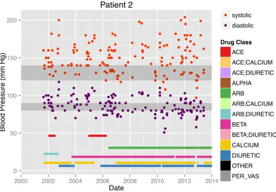
antihyperten-sive medication classes. . . 24 2-6 Example patient: dense, noisy blood pressure measurements and many

antihypertensive medications. . . 25 2-7 Distribution of blood pressure measurements in patient study population. 26 2-8 Duration of blood pressure measurement history in selected patient

population. . . 27 2-9 Weight and BMI measurement for two example patients. . . 27 2-10 Distribution of weight and BMI measurements in selected patient

pop-ulation. . . 28 2-11 Distribution of patient count by antihypertensive drug class prescribed 29 2-12 Distribution of patient count, by antihypertensive drug class and

cu-mulative length of drug prescriptions. . . 30 3-1 Dendrogram for hierarchical clustering on blood pressure features . . 34 3-2 Clustering on blood pressure features: cluster sizes . . . 35 3-3 Final selection of (normalized) blood pressure variables for clustering:

A-1 Start bin: 140+, CART classification . . . 59 A-2 Start bin: 140+, RF classification . . . 60 A-3 Random Forest classification for cluster 6 in <120 starting bin: variable

importance for decreasing node impurity . . . 63 A-4 Random Forest regression for cluster 6 in <120 starting bin: variable

List of Tables

1.1 Hypertension definitions from JNC 7 report . . . 14 1.2 Notes for demographic sub-populations from the JNC 7 report [2] . . 15 1.3 Complementary approaches: medical studies vs. analytics on EHR . . 16 2.1 Antihypertensive drug classes, as used in this work . . . 28 3.1 Feature creation: options for summarizing temporal data . . . 32 3.2 Blood pressure features used for clustering . . . 35 3.3 Cluster descriptions, plus trends by cluster for features not used in

cluster creation. . . 36 4.1 Non-blood-pressure features, used (or tried) as independent variables

for prediction . . . 41 4.2 Out-of-sample results: cluster by blood pressure features to create

de-pendent variable, predict cluster using non-blood-pressure features. . 43 4.3 Out-of-sample results: subset or group blood pressure clusters to create

dependent variable for predictive models . . . 44 4.4 Out-of-sample results: cluster by blood pressure features, split, predict

cluster in each segment . . . 46 4.5 Out-of-sample results: group (rather than cluster) by systolic blood

pressure, predict group using other features . . . 47 4.6 Count of patients, segmented by initial and final blood pressure (75%

4.7 Out-of-sample results: predict final blood pressure, segmented by start-ing blood pressure . . . 49 5.1 Feature importance for prediction: general trends from Sections 4.2

and 4.3, using CART, RF, and linear/logistic regression. . . 52 A.1 Start bin: 140+, logistic regression (w/ sequential removal of high

p-value variables) . . . 58 A.2 Best results for segmenting by initial blood pressure, clustering within

each segment, and then predicting final-year blood pressure for each bin-cluster sub-group. (“class.” is model accuracy minus baseline ac-curacy, “regress.” is R2_{) . . . . 62}

B.1 Results for predicting blood pressure trajectory separately for diabetic and non-diabetic patients . . . 66

Chapter 1

Introduction

1.1

Motivation

High blood pressure, or hypertension, is one of the major public health issues facing the world today. Of US adults, age 20 or older, 78 million, or 33% have hypertension, and only 53% of them have it controlled [4]. An additional 30% of the population is prehypertensive [5]. Worldwide, 40% of the over-25-year-old population has hy-pertension: with frequency ranging from 35% in the Americas to 46% in Africa [10]. High blood pressure increases the risk of myocardial infarction, heart failure, stroke, and kidney disease. In fact, the risk doubles for every 20 mm Hg systolic or 10 mm Hg diastolic increase, starting at 115/75 mm Hg (top end of “normal” range) [2]. Currently 1 in 3 deaths worldwide (17 million annually) are due to cardiovascular disease [10, 9]. The US spends an estimated $46.4 billion annually on the direct and indirect costs of hypertension [4]. The World Health Organization projects lost output due to cardiovascular disease for low and middle-income countries at approximately 2% of GDP in the years 2011 to 2025 [10].

1.2

Current Treatment Guidelines

In 2003, the seventh Joint National Committee on Prevention, Detection, Evalua-tion, and Treatment of High Blood Pressure (JNC 7) issued a report reviewing and

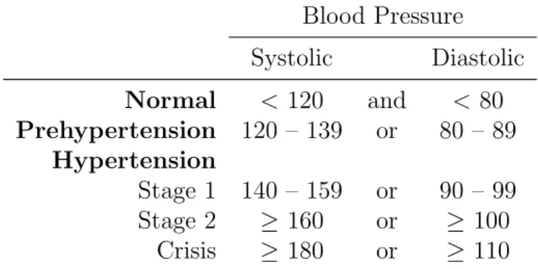
Blood Pressure Systolic Diastolic Normal < 120 and < 80 Prehypertension 120 – 139 or 80 – 89 Hypertension Stage 1 140 – 159 or 90 – 99 Stage 2 ≥ 160 or ≥ 100 Crisis ≥ 180 or ≥ 110 Table 1.1: Hypertension definitions from JNC 7 report

summarizing evidence and expert consensus into a concise guide for use by clinicians [2, 1]. In late 2013, multiple organizations released updated guidelines [7, 6, 11, 3]. While many aspects of these recent guidelines agree, with each other and the JNC 7 report, their differences highlight the uncertainty in best-practice for hypertension treatment [13].

Key points of the JNC 7 guidelines are: 1. Hypertension definitions as in Table 1.1.

2. Lifestyle modifications recommended for patients with prehypertension: weight reduction (if overweight or obese), adoption of a DASH diet (Dietary Ap-proaches to Stop Hypertension), sodium reduction, increased physical activity, and moderation of alcohol consumption.

3. For hypertensive patients, treatment with medication (see Table 2.1) is advised (in addition to lifestyle modifications).

4. Patients should generally start with a thiazide diuretic, ACE inhibitor, ARB, calcium-channel blocker or β-blocker. Adjust treatment approximately monthly, until blood pressure goal is reached. Adjustments include increasing dosage, and adding or substituting an additional drug from the classes above.

5. Typically, patients will require two or more medications to achieve blood pres-sure control.

Prevalence Treatment Minorities “Blood pressure control rates

vary in minority populations and are lowest in Mexican Americans and Native Americans.”

“In general, the treatment of hy-pertension is similar for all de-mographic groups, but socioeco-nomic factors and lifestyle may be important barriers to BP con-trol in some minority patients.” Blacks “The prevalence, severity, and

impact of hypertension are in-creased in blacks.”

“... somewhat reduced BP re-sponses to monotherapy with β-blockers, ACE inhibitors, or ARBs compared with diuretics or CCBs [...] largely eliminated by drug combinations that in-clude adequate doses of a di-uretic.”

Over 65 “Hypertension occurs in more than two thirds of individuals af-ter age 65 years.1 This is also the population with the lowest rates of BP control.”

“... follow the same principles outlined for the general care of hypertension. [...] lower initial drug doses may be indicated to avoid symptoms; however, stan-dard doses and multiple drugs are needed in the majority ...” Women “Oral contraceptives may

in-crease BP and the risk of hyper-tension increases with duration of use [...] hormone replacement therapy does not raise BP.”

Table 1.2: Notes for demographic sub-populations from the JNC 7 report [2]

Adjustments are recommended for certain patients. The JNC 7 report includes a table of “compelling indications” for which the use or avoidance of particular drug classes is advised: heart failure, post-myocardial infarction, high coronary disease risk, diabetes, chronic kidney disease, and recurrent stroke prevention. Other comorbidities with special treatment notes include: pregnancy, asthma, gout, history of significant hyponatremia, reactive airways disease, second or third-degree heart block, history of angioedema, and high potassium levels. Notes for demographic-based sub-populations are collected in Table 1.2.

Table 1.3: Complementary approaches: medical studies vs. analytics on EHR Randomized controlled trials and

prospective studies

Analytics on existing electronic health records (EHR)

Pros Gold standard:

• Statistical controls

• High-quality data collection

• Larger study population

• Potentially longer patient history • Flexibility in models and

ques-tions considered Cons • Expensive, limits size of study

population

• Limited insight for sub-populations and questions not included in study design

• Missing information • Messier data

1.3

Research Goals

From Sections 1.1 and 1.2, it is clear that improvements in the treatment of hyperten-sion would have a major impact, and there is disagreement and uncertainly in current evidence-based guidelines. Furthermore, experimentation is typically required to find an effective treatment for a given patient. We propose a complementary approach of applying analytics to patient electronic health record (EHR) data to accomplish one or more of the following goals:

1. Find conjectures parallel, and potentially orthogonal, to current treatment guidelines.

2. Hasten patient response time to therapy. 3. Optimize therapy selection.

Table 1.3 summarizes the benefits and drawbacks of this approach.

This thesis represents progress towards these goals. Most notably, the clusters described in Section 3.2 and the interpretation of the models in Chapter 4 reveal a number of known clinical trends – fulfilling the first part of goal one. This research has not yet clearly identified conjectures orthogonal to current guidelines. A pre-dictive model of blood pressure trajectory is a key enabler for meeting these goals.

Such a model, if interpretable, might suggest treatment plans not common in cur-rent clinical practice, thereby meeting the second half of goal one, and hopefully goal two. Furthermore, good understanding of the factors influencing blood pressure tra-jectory, provided by a predictive model, is a prerequisite to the optimization model suggested by goal three. Creating a predictive model of blood pressure trajectory first requires a quantitative, data-based definition of blood pressure trajectory. The majority of this thesis is, in effect, spent grappling with this definition. Section 3.2 presents intriguing, clinically-relevant patient clusters, discovered by clustering on blood-pressure-related variables. Section 4.2 describes numerous attempts to trans-late this insight to prediction: using such clusters as the dependent variable of a predictive model. Unfortunately, the predictive power of these models is almost en-tirely due to differentiating patients with overall low versus high blood pressure – information already available to a physician after a patient’s initial visit. Finally, we developed the models described in Section 4.3, which do predict blood pressure changes in a clinically-relevant way. While the performance of these models is cur-rently modest, there is potential in refining them further, as discussed in Section 5.3.

1.4

Structure

The structure of this thesis is as follows. Chapter two describes the data set: source, inclusion criteria, visualizations of example and aggregate data, and cleaning and preprocessing steps taken. Chapter three discusses feature selection as well as the re-sult of clustering on select blood pressure features: clinically-relevant patient groups. Chapter four presents models and results for predicting blood pressure trajectory, over three spirals of development. Chapter five notes general trends, followed by concluding remarks and suggestions for future continuation of this work.

Chapter 2

Data

2.1

Boston Medical Center

This work is enabled by access to anonymized data from the Boston Medical Center (BMC), a 496-bed academic medical center, affiliated with Boston University School of Medicine, and located in Boston’s South End. BMC provides pediatric and adult care, including primary and family medicine, advanced specialty care, and trauma and emergency services. It is the largest safety-net hospital in New England. Available anonymized data comes from: up to 15 years of EHR (including visit history, vital signs, diagnoses, problem list, lab results, and prescriptions), billing data, demograph-ics, and cancer registry information. Provider notes as well as diagnostic images and signals are not available. The anonymized data is linked by unique identifier numbers assigned to each patient and provider.

2.2

Patient Inclusion Criteria

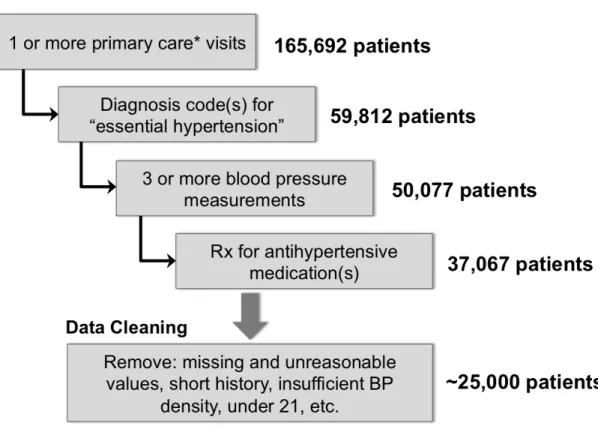
Figure 2-1 shows the patient inclusion criteria for this analysis. We chose these criteria to select patients interacting with the BMC system regularly, without a known cause for their hypertension, and with sufficient blood pressure and medication information to address the goals stated in Section 1.3. We set aside a random 25% of these patients for eventual out-of-sample testing set. This data was not used at all in the

Figure 2-1: Patient inclusion criteria

analysis described in Chapters 3 and 4. The remaining 75% was used for training and validation.

Further filtering included steps such as removing missing and unreasonable values, requiring a minimum number, duration or density of blood pressure measurements, and excluding children. Several variants of such filtering were used throughout the analysis described in Chapters 3 and 4. In all cases, approximately 25,000 patients remained.

2.3

Data Fields

The EHR data fields used in this analysis are: date of birth, race, sex (demograph-ics); blood pressure, weight, height, BMI (vitals); and antihypertensive medication prescriptions. All of these fields, except demographics, have a temporal element with irregular measurement intervals. The challenge of transforming this data into

vari-0 5000 10000 15000 female male Sex 0 5000 10000

black whitehispanicasian otherunknown

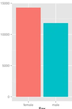
Race Figure 2-2: Distribution of sex in selected patient population.

ables for exploratory and predictive analytics is discussed in Section 3.1

2.3.1

Demographics

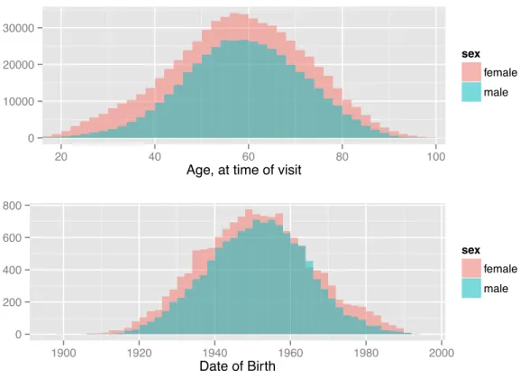
Patient sex is directly available in the EHR. A histogram for the patient population described in Section 2.2 is shown in Figure 2-2. Age at time of visit is easily calculated from date of birth1. Histograms for both values are shown in Figure 2-3. Note the greater proportion of women in the age plot, and that the date-of-birth plot counts patients while the age plot counts visits: women visit the doctor more often than men. A number of race codes exist in the EHR. Same-race codes were combined (e.g. ”DEM|RACE:a”, ”DEM|RACE:asian”, ”DEM|RACE:or”, and ”DEM|RACE:oriental” all correspond to asian). The few patients coded as hispanic/black or hispanic/white were included in both categories. Codes for indian, middle eastern, native american, asian pacific islander, aleutian, eskimo, and multiracial were infrequent or nonexistent. These patients were combined with those coded as “other”. See Figure 2-4 for the

0 10000 20000 30000

20 40 60 80 100

Age, at time of visit

sex female male 0 200 400 600 800 1900 1920 1940 1960 1980 2000 Date of Birth sex female male

Figure 2-3: Distribution of patient age at time of visit, and birth-date, in selected population.

0 5000 10000

black white hispanic asian other unknown

Race

sex

female male

resulting distribution.

2.3.2

Blood pressure

Blood pressure is measured in millimeters of mercury (mm Hg). It is typically re-ported as systolic pressure (pressure in arteries when heart contracts) over diastolic pressure (pressure in arteries between contractions). Others ways to report blood pressure are pulse pressure (systolic minus diastolic) and mean arterial pressure (av-erage pressure throughout a heartbeat cycle). Mean arterial pressure can be estimated by: 2/3 diastolic + 1/3 systolic.

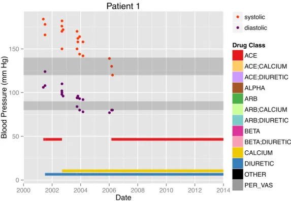
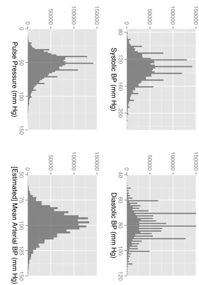
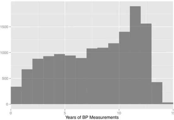
The EHR includes systolic and diastolic blood pressure measurements. While a few of these are specifically marked as measured with patient lying, sitting, or standing; most are coded as “unknown”. Values greater than 300 mm Hg were removed to exclude obviously erroneous values. Of interest for this research is the trajectory of a patient’s blood pressure over time. For some patients, such as the example in Figure 2-5, this trend is fairly clear. More commonly, the variation in blood pressure measurements is greater than any increasing or decreasing trend. The patient in Figure 2-6 is such an example. Summarizing blood pressure trajectory is further discussed in Chapters 3 and 4. Figure 2-7 indicates the distribution of blood pressure measurements for the study population, by all four metrics described above. Note the “comb” pattern, suggesting doctors often round to the nearest increment of 5 or 10 when taking a reading. Figure 2-8 plots the duration of patient measurement history (difference between date of first and latest blood pressure measurement on record). The drop-off around 13 to 15 years is likely due to the phase-in of electronic record keeping at BMC.

2.3.3

Weight and BMI

Both weight and BMI are available in the EHR. They are typically less noisy than the blood pressure measurements, making trends clearer. Figure 2-9 shows these measurement for the same patients as in Figures 2-5 and 2-6. Figure 2-10 shows the

● ● ● ● ● ● ● ● _● ● ● ●● ● ● ● ● ● ● ●● ● ● ● ● ● ● ● ●●●● ● ● ● ●●● 0 50 100 150 2000 2002 2004 2006 2008 2010 2012 2014 Date Blood Pressure (mm Hg) ● ● systolic diastolic Drug Class ACE ACE;CALCIUM ACE;DIURETIC ALPHA ARB ARB;CALCIUM ARB;DIURETIC BETA BETA;DIURETIC CALCIUM DIURETIC OTHER PER_VAS Patient 1

Figure 2-5: Example patient: clear blood pressure trajectory, three antihypertensive medication classes.

distribution of these measurements in the study population. Informed by exploratory scatter plots, erroneous data and extreme outliers were excluded by limiting data to: weight between 25 and 600 kg, height between 130 and 250 cm, and BMI between 10 and 75. Additional issues and solutions related to these fields are discussed in Section 5.3.1.

2.3.4

Antihypertensive Medications

Medication usage is reflected in the EHR by an entry every time a doctor writes or updates the prescription. Each entry includes an RxNorm[8] code that uniquely identifies the medication, the start date of the prescription, the end date of the prescription (typically the start date of the next entry for the same drug), dosage instructions (e.g. “take one by mouth once daily”), the drug name (e.g. “benazepril 5 MG / Hydrochlorothiazide 6.25 MG Oral Tablet (Lotensin HCT) (RXCUI:207881) (RXCUI:207881)”), the number of pills (or other units) per refill, and the number

● ● ● ●● ● ● ● ● ● ● ● ● ● ● ● ● ● ● ● ● ● ●●● ● ● ● ● ● ● ● ● ● ● ● ● ● ● ● ● ● ● ● ● ● ● ● ● ● ● ●● ● ● ● ● ● ● ● ● ● ● ● ● ● ● ●● ● ● ● ● ● ● ● ● ● ●● ● ● ● ●● ● ● ● ●● ● ● ● ● ●● ● ● ● ● ● ● ● ● ● ● ● ● ● ● ● ● ● ● ● ● ● ● ● ● ● ● ● ● ●● ●● ● ● ● ● ● ● ● ● ● ● ● ● ● ● ● ● ● ● ● ● ● ● ● ● ● ● ● ● ● ● ● ●● ● ● ● ●●● ● ● ● ● ● ● ● ● ● ● ● ●● ●● ● ● ● ● ● ● ● ● ● ● ● ● ● ● ● ●● ● ● ● ● ● ● ● ● ● ● ● ● ● ● ● ● ● ● ● ● ● ● ● ● ● ●●● ● ● ● ● ●● ● ● ● ● ● ● ●● ●●●● ●● ● ● ● ● ● ● ● ● ● ●●● ● ● ● ● ● ● ● ● ● ● ● ● ● ● ● ● ● ● ● ● ● ● ● ● ● ●● ● ● ● ● ● ● ● ●● ● ● ● ● ● ● ● ● ● ● ●●● ● 0 50 100 150 200 2000 2002 2004 2006 2008 2010 2012 2014 Date Blood Pressure (mm Hg) ● ● systolic diastolic Drug Class ACE ACE;CALCIUM ACE;DIURETIC ALPHA ARB ARB;CALCIUM ARB;DIURETIC BETA BETA;DIURETIC CALCIUM DIURETIC OTHER PER_VAS Patient 2

Figure 2-6: Example patient: dense, noisy blood pressure measurements and many antihypertensive medications.

of refills. We assume the patient is taking a drug the entire time between the listed start and end dates. As antihypertensive class is the clinically-relevant factor [2], we are able to simplify the 601 RxNorm codes (75 drug names) by grouping them into the classes in Table 2.1. Single-pill combination drugs are split into both relevant classes. Obtaining dosages required parsing the, relatively unstructured, instruction field to extract the number of pills per day2 and drug name to extract milligrams per pill (or unit). Currently, this parsing captures dosage for 92% of the prescription entries. Additional processing to further utilize available drug data is discussed in Section 5.3.1.

Figures 2-5 and 2-6 show antihypertensive drug prescriptions for two example patients. Note, the classes here reflect the organization for the EHR database before additional sorting. One-pill combos are the legend entries with colons. Figures 2-11 and 2-12 show statistics of drugs prescribed, after sorting into the classes of Table 2.1.

0

50000

100000

150000

80

120

160

200

Systolic BP (mm Hg)

0

50000

100000

150000

0

50

100

150

Pulse Pressure (mm Hg)

0

50000

100000

150000

40

60

80

100

120

Diastolic BP (mm Hg)

0

50000

100000

150000

50

75

100

125

150

[Estimated] Mean Ar

ter

ial BP (mm Hg)

0 500 1000 1500 0 5 10 15 Years of BP Measurements

Figure 2-8: Duration of blood pressure measurement history in selected patient pop-ulation. weight (kg) BMI weight (kg) BMI Patient 1 Patient 2 30 60 90 120 2002 2004 2006 2008 2010 2012 2002 2004 2006 2008 2010 2012 Date Measurement V alue

0 10000 20000 10 20 30 40 50 60 70 BMI sex female male 0 20000 40000 0 100 200 300 400 500 Weight (lb) sex female male

Figure 2-10: Distribution of weight and BMI measurements in selected patient pop-ulation.

1 Thiazide diuretics

2 Other diuretics (loop, potassium-sparing, aldosterone-receptor blockers, carbonic anhydrase)

3 Angiotensin-converting enzyme (ACE) inhibitors 4 Angiotensin II receptor blocker (ARB)

5 Calcium channel blocker (CCB) 6 α-Blockers

7 β-Blockers

8 Centrally acting adrenergic agents Less common:

9 Peripheral vasodilators 10 Hydralazine hydrochloride

11 Minoxidil

12 Reserpine

0 2000 4000 6000 8000 ACE THIAZIDE BET A CALCIUM DIUR_nonTHIAZ ARB ALPHA CENTRAL_A CT Hydr alazine_HCl Mino xidil Reser pine PER_V AS Figure 2-11: Distribution of patien t coun t b y an tih yp ertensiv e drug class pre sc rib ed

A

CE

THIAZIDE

BET

A

CALCIUM

DIUR_nonTHIAZ

ARB

ALPHA

CENTRAL_A

CT

Hydr

alazine_HCl

Mino

xidil

Reser

pine

PER_V

AS

0

500

1000

1500

2000

0

500

1000

1500

2000

0

500

1000

1500

2000

0

5

10

15

0

5

10

15

0

5

10

15

0

5

10

15

Total Y

ears on Dr

ug (b

y P

atient)

Chapter 3

Data Exploration

3.1

Feature Creation

As mentioned in Section 2.3, one of the main challenges of this research was deter-mining the best way to summarize temporal data with variable measurement density and spacing, start date, and length of history. Table 3.1 presents the various op-tions considered. Note the use of residual standard error1 _{rather than R}2 _{to indicate}

goodness of fit. Values of R2 near zero can indicate noisy data or a poor fit, but also correspond to a good fit of nearly constant data: a common pattern for blood pressure and weight. The use and evaluation of these features for data exploration and prediction is discussed in Section 3.2 and Chapter 4.

3.2

Blood Pressure Trajectory Clusters

One way to explore and evaluate the features presented in Section 3.1 is through clustering. First we discuss general preprocessing done, or tried, over the course of experimenting with various features, followed by details on the features ultimately selected for clustering.

Clustering algorithms operate on distances between data points, so the data must first be normalized, and possibly transformed. For example, the non-negative, skewed

Blood Pressure (very noisy) Mean, median, standard deviation

Number, density (and timespan) of measurements Polynomial fit:

• Linear: intercept, slope • Quadratic: 3 coefficients • Residual standard error (RSE) • Value of fit at t0

• Differences between 1st and 2nd order fit Weight and BMI

Mean, median, standard deviation Linear fit: intercept, slope, RSE Medications, by drug class

Binary (after threshold for minimum script duration?) Count of scripts

Cumulative script duration

Fraction of time: cumulative script duration / timespan Max dose, pills/day, times/day

Use of two or more classes: • Pairwise, triplet, etc.

• Full combination (e.g. sort and consider top 30 combinations, plus ”other”) Time period considered

Entire patient history

Divide into discrete segments

Initial window (and final window), remaining record

distribution for residual standard error is more symmetric after a ln() transform. When fitting blood pressure, weight, and BMI with a linear or quadratic equation, the slope and curvature coefficients for most patients are close to zero. Therefore, patients with larger values of these coefficients, often correlated with shorter mea-surement history, tend to dominate any clustering algorithm. The neglog transform [12], sign(x) + ln(|x| + 1), can be used to temper this effect. It is nearly linear close to zero, while pulling in extreme positive and negative values.

After applying transformations to some variables, we normalized all non-binary variables by subtracting the mean and dividing by the standard deviation. We then experimented with hierarchical, k-means, and spectral clustering, as well as weighting select variables to increase their influence. We first tried clustering on all non-drug variables, with the idea of then comparing medication usage by cluster. With so many variables, the clusters were hard to interpret. No striking drug trends emerged.

Next, we tried clustering with only blood pressure features, aiming to discover the best way to quantify “blood pressure trajectory” from the multitude of possible features listed in Table 3.1. We found hierarchical clustering with 8 clusters produced sensible, interpretable clusters. We then pared down the features used, while checking that the cluster distinctions remained. The seven blood pressure features ultimately used are presented in Table 3.2. Figure 3-1 shows the hierarchical clustering den-drogram, with a red box indicating the choice of 8 clusters. Figure 3-2 shows the resulting cluster sizes.

Each plot in Figure 3-3 shows one of the features used for clustering: a boxplot of its normalized values, separated along the x-axis by cluster. We studied this plot to determine a description for each cluster, which we present in the left column of Table 3.3. For example, consider Cluster 6. The median.sys and median.dia plots show that patients in this cluster tend to have lower systolic and diastolic blood pressures than the population average (indicated by the black line at zero). By considering the unnormalized, population average and standard deviation of median blood pressure, listed on the right of Figure 3-3, we further note that the middle 50% of Cluster 6 patients have median systolic blood pressure between approximately 120

Figure 3-1: Dendrogram fo r hierarc h ical clustering on blo o d pressure features

Name Description

1 median.sys median systolic blood pressure 2 median.dia median diastolic blood pressure

3 B1.lin.sys linear fit of systolic blood pressure, β1 coefficient (slope)

4 B1.lin.dia linear fit of diastolic blood pressure, β1 coefficient (slope)

5 B2.quad.sys.negLog quadratic fit of systolic blood pressure, β2coefficient

(cur-vature), transformed by: sign(x) + ln(|x| + 1)

6 B2.quad.dia.negLog quadratic fit of diastolic blood pressure, β2 coefficient

(curvature), transformed by: sign(x) + ln(|x| + 1) 7 BPdensity total number of visits with blood pressure measurement

divided by years between first and latest measurement All features calculated by patient, over patient’s entire measurement history.

Table 3.2: Blood pressure features used for clustering

0 1000 2000

1 2 3 4 5 6 7 8

Cluster

Characterization of cluster Variables not used for clustering – trends by cluster

1 Ok now, slowly getting in trou-ble

Younger, monotherapy (especially thi-azide), heavier (gradual weight gain?) 2 Low and stable Lighter, least noisy BP, more non-black

men, tried 1-3 drugs (more non-thiazide diuretics)

3 Positive curvature, rapid de-crease

Shorter history, losing weight, slightly older

4 High and stable, noisy Heavier, noisy BP, tried several drugs (less non-thiazide diuretics), more blacks 5 Negative curvature, rapid

in-crease

Shorter history, gaining weight, monother-apy or no drugs

6 Dense measurements, low and stable

Heavier, slightly older women, noisy weight/BMI, tried many drugs

7 Stable, elevated diastolic, least dense measurements

Heavier, younger, thiazide: alone or with one other class (less non-thiazide diuret-ics), more blacks

8 Low diastolic, elevated systolic Older, more non-black women, tried many drugs

Table 3.3: Cluster descriptions, plus trends by cluster for features not used in cluster creation.

and 133 mm Hg and diastolic between 70 and 80 mm Hg: values corresponding to the low end of the prehypertension range. Next, looking at the B1.lin.sys, B1.lin.dia, B2.quad.sys.negLog, and B2.quad.dia.negLog plots, features which have unnormal-ized population mean close to zero, shows that the slope and curvature of blood pressure for Cluster 6 patients is typically close to zero. Finally, the BPdensity plot reveals that Cluster 6 patients have their blood pressure measured more frequently, on average, than patients in other clusters. Therefore, as shown in Table 3.3, we label this cluster, “Dense measurements, low and stable.”

We then made plots similar to Figure 3-3 of features not used for clustering. Notable trends in these features are recorded in the right column of Table 3.3. These additions to the cluster descriptions are clinically-consistent with the

blood-pressure-● ● ● ● ●● ● ● ●●●● ●● ● ● ● ● ● ● ●● ● ● ●● ●●●● ●●● ●● ● ●●● ● ●● ● ●●●●●● ●● ● ● ●● ● ●●● ●● ● ● ● ●● ● ● ●●● ●● ●●● ● ●● ●●●●●●●● ● ●●●●●● ●●●●●● ●●●● ● ●●●● ● ●●● ● ● ● ● ●●● ● ● ● ● ●● ● ●●●●●● ● ● ● ● ● ●● ● ●● ●●●● ● ● ● ● ● ●● ● ●● ●● ●●● ●●● ● ● ●●●●● ●● ●●● ● ●●●● ●●● ●●●●●●●●●● ● ●●● ● ● ● ●● ●●● ● ● ●● ●●●● ● ●● ● ● ● ● ●● ●●● ●●●● ●●● ●● ● ●●● ●●●●●●● ●● ●● ●●●●●●●●● ● ●● ● ● ●●●● ●●● ●● ● ● ● ●●●●●●●●●●●● ●●●● ● ● ● ● ● ● ●● ● ●● ●●● ● ● ● ●●●●●●● ●● ●●●●● ●●●●●● ●●●●●● ●●●●● ● ●● ● ●●●● ●●● ●● ● ● ● ● ● ●● ● ●● ● ●● ● ●●●●●●●●●●●●● ●●● ●● ● ● ● ● ● ●●● ● ●●● ●●●● ●● ● ● ● ● ● ● ●●● ●●●●● ● ● ● ● ● ●● ●●●●● ●●●●●●●●●● ● ●● ●●●●●●● ● ●●●● ● ●● ●●●●● ●● ●● ●●●●●●● ●●●●●●●●● ●●●●●● ●● ● ●●● ●● ●●● ●●● ●● ●● ● ● ● ● ● ●● ●● ● ●●● ●●● ●●●● ●● ●●●●●●● ●●●●●●● ● ● ●● ●● ● ● ● ● ●● ●●●●● ●● ● ● ●● ●●● ●●● ●●●● ●●●● ●● ●● ●● ●●● ● ●● ●●●●● ● ●● ●●●●● ●●● ● ● ● ●● ● ● ● ● ● ●● ●●● ●●●●● ● ● ● ●● ● ● ● ● ●●● ●●● ●● ● ●● ●● ●● ●● ●●●●● ●●● ● ● ●●● ● ●● ● ●● ●● ● ●● ●● ● ●● ● ●●●●● ●●●● ●● ●●●●●● ●●●● ● ●●●● ●●●● ● ● ● ●● ● ● ●●●●●● ●● ● ● ●●●● ● ● ●● ●● ●●● ●● ● ●●● ● ●● ●● ●●● ●● ●●●●●● ●●● ● ●●●● ●●●●● ● ● ● ● ● ● ● ●●●● ● ●● ● ●● ● ●●● ●● ●●●●●● ● ●●●●●●●●●●●●●●●●●●●● ● ● ● ● ● ●●●●●● ●●●●●●●●●●●●●●●●●● ●●●●●●●● ● ●● ●●● ●●● ●●●●● ●●● ● ●● ●● ● ●●● ●● ●● ●●●●● ●●● ●●●●●● ●● ●●●●●● ●● ●●●● ● ●●●●●●●●●●●●●●●●● ● ● ● ● ● ● ●● ● ● ●● ● ● ● ●● ●●●●●●●●●●●●●●●●●●●●●●● ●●●●●●●●●●●●●●●●●●●●●● ●●●●●●● ●●●●●●●●●●● ●●●● ●●●●●●●●●●●●●●●●●●●●●●●●●●●●●● ● ● ●●●●●●●●● ● ●● ● ● ● ● ●● ● ●●● ● ● ●● ● ● ●● ● ● ●●●● ●●●● ● ●●● ● ● ● ● ●● ● ●● ● ●● ● ● ● ● ● ● ● ● ●● ● ●● ● ● ● ● ● ●● ● ●● ●●● ●● ●●●●●● ●● ● ●●●● ●● ●● ● ● ● ● ●●●●●●●● ●●●● ●●●●●●●●●●●●●● ●●●●●●●●● ●● ●●●●●●●●●●●●●●●● ●●●●●●●●● ●● ●●● ● ● ● ● ● ● ● ●● ●●● ●● ● ●● ●● ●●● ●●●● ● ● ●● ● ● ● ● ●● ●●●●●●●● ● ●●●●● ●●● ●●●● ● ● ●● ● ●●●●●●●●●●●● ●●● ● ●●● ● ● ● ● ●● ●●●●● ● ● ●● ●● ● ● ● ● ●●●●●●●●● ●●●●● ●●●●●●●● ●● ●●● ● ● ●●●● ● ● ● ● ● ● ●●●● ● ●●●●●●●● ●●● ● ●●● ●●●●●●● ● ●● ● ● ●● ● ●●● ●● ● ● ● ● ●● ●●●●●●● ●● ●● ● ● ●● ●●● ● ●● ●● ● ● ●●●●●● ●● ●● ● ● ● ● ● ● ● ●●●●●● ●● ●●● ●●●● ● ●● ●●●● ●● ● ●● ● ● ● ● ● ● ●●●●●●●●● ●●● ●● ●●● ●●● ●● ● ●● ● ●● ●●●●●●●● ●●●● ●●● ● ●● ● ● ● ● ● ● ● ●●● ●●●●● ● ● ● ●● ●● ● ●● ● ●● ●●●● ●● ●● ●●● ● ● ● ●●● ●● ●● ●●● ● ● ● ● ●● ●● ●● ●●●●● ● ● ● ● ● ● ● ● ●● ●●●●●●● ●●● ●●●●● ●●● ●●●● ●●●●●●●● ●●●●●●●●●● ●●●●●●●●●● ●●●● ●● ● ●●●●● ●●●●●●●●●●●●●●●●●●●●●●●●●●●●●●●●●● ● ● ● ●●●● ● ● ●●●● ●● ● ● ● ●● ●●● ● ●● ● ● ●● ●● ● ● ● ●● ● ● ●●●●●●●●● ●●●●● ●●● ●●● ●●● ●●●●●●●●● ●● ● ● ● ● ●● ●● ●●●●● ●●●●●●●●●● ● ●●● ●●●● ● ●●●●● ● ●●●●●●●● ●● ●● ●●●●●●● ●●●●●●●●● ●●●●●● ●● ● ●●● ●● ●●● ●●● ●● ●● ● ● ● ● ● ●● ●● ● ●●● ●●● ●●●● ●● ●● ●●●●●●●●●●●● ● ● ●● ●● ● ● ● ● ●● ●●●●● ●● ● ● ● ● ●●● ●●●● ●●●● ●●●● ●●●●● ●●● ● ●● ●● ●●●● ● ●● ●●●●●● ●● ●●●● ● ● ● ● ● ●● ●●● ●●●●● ● ● ● ●● ● ● ● ● ●●● ●●● ●● ● ●● ●● ●● ●● ●●●●● ●●● ● ● ●●● ● ● ● ●● ●● ● ●●●● ● ● ●● ● ●● ● ●●●●● ● ●● ●●●●●● ●●●● ● ●●●● ●●●● ● ● ● ●● ● ● ●●●●●● ●● ● ● ●●●● ● ● ● ● ●● ●●● ●● ● ●●● ● ●● ●● ●●● ●● ●●●●●● ●●● ● ●●●● ●●●●● ● ● ● ● ● ● ● ●●●● ● ●● ● ●● ●● ●● ●● ●●●●●● ● ●●●●●●●●●●●●●●●●●●●● ●● ●● ● ● ● ● ●●● ● ●● ● ●● ●● ●●●●●● ●●●● ●●● ●●●● ● ●● ●●●● ●● ●●● ●●●● ● ●● ●●●● ●●●● ●●● ●● ● ● ● ●●● ●●●● ●●● ●●●●●●●●●● ●●●● ●●●●● ●●●●●●●● ● ●●●●●●●●●●●●●●● ●●●● ●●●●●●● ● ● ●●●●●●●●●●●● ●●●●●●●●● ●●●●●●● ●●● ●● ●● ●●●●●● ●●● ●●● ●●●●● ●●●●● ●●●●●●● ●●●●●● ●●●●●●●●●●● ●●●●●●●● ●●●● ●●●●●●●●●●●●●●●●●●●●●●●●●●●●●●●●●●●●●● ●●● ●●● ●●●● ●● ●●●● ●●●● ●● ●● ●●●●●●●●●●●●●●●●● ●●●●●●●●●●●●●●●●●●●●●●●●●●●●●●●●● ● ● ● ● ● ● ● ● ●● ● ● ● ●●●●●●● ● ●● ●●●●●● ● ●●●●●●●●●●●●●● ●●●●● ●●●● ● ●●●●●●●●●● ●●●●● ●●● ●●● ●●●●●●●●●●●●●●●●●●●●●●●●●●●●●●●●●● ●●● ●● ●● ●●●●●● ●●●●●●●●● ●●●●●●● ● ●●●●●●● ●●● ●●●●●●●●●●●●●●●●●●● ● ● ● ● ● ● ● ● ● ● ● ●●● ● ●●●●●● ●●● ●● ●●● ● ●● ● ● ● ●● ●● ● ●●● ●●● ●● ●● ●●●●●●●● ● ● ●● ●● ● ● ● ● ● ● ●●●●● ●● ●●●● ●● ● ●●● ●● ●●●●●● ●●●●●●●●●●●●●●●● ● ●●●●●●●●●● ●●● ●● ● ● ● ● ● ● ● ● ●●●●●● ●●●● ● ●●●● ●●●●●●● ● ● ●● ● ● ● ● ● ●● ●● ●●●●● ● ●●●●●●●●● ●● ●●● ● ● ● ●●●● ●●● ●●● ● ● ● ● ●●●● ●●● ● ●●●●●● ●●●●●● ●●● ●●●●●●● ●●●●● ●●● ●●●●●●●● ●●● ●● ●●●●●●●●●● ●● ●●●●●●●●● ●●●●●●● ●●●●●● ●●●● ●●●●●●●●●● ●●●●●●● ●● ● ● ● ● ● ● ● ● ● ●●● ●● ●● ●● ●●●●●● ●●●● ●●● ● ● ● ● ● ●● ● ●●● ●● ●● ● ● ●● ●●●●●●● ● ● ●●●●●● ●●● ●●●●● ● ● ● ●● ●●●● ●●●●●●●●●●● ● ●●●●● ●●●●●●● ●● ●●●● ●● ● ●●●●●●● ●●●●●●●●●●●●●●●●●●●●●●●● ●●●●● ●●●●● ●●●●●●●●●● ●●●●●●●●●●●●●●●●● ● ● ●● ● ●●●●●●●●● ● ● ● ●● ●●● ●●●●●●●● ●●●●● ●●●●●● ● ●● ●●● ●● ● ● ● ●● ●● ● ● ● ● ●● ● ● ●●●●● ●●● ● ●●● ●●●● ●●● ● ●● ● ● ●●●●●●●●●●●●●●●●●●● ● ● ●● ● ● ●●● ●●● ●● ● ●● ●●●● ● ●● ● ●● ●● ●●●●●●●●● ●● ●●● ●●● ● ●● ●●●● ●●●●●●● ● ●●●●●●●●● ●● ●●● ● ● ● ● ● ● ● ● ● ●●●● ●●●●●●●●● ●● ●● ●● ● ●●●●●●●●●●●●● ●●● ● ●●● ●●●● ● ●●●● ●●●●●●● ●● ● ● ●● ●●●●●●● ●●●●● ●● ●●● ● ●●●●● ● ● ● ●●●●●●●● ●● ●● ●● ●●●●●●●● ●● ●●●● ●● ●●●● ●●●●●● ●● ●●●●●●●●● ●●●●●●●● ● ●● ●●●●●● ●●●●●●●●● ●●●● ● ●●●● ●●●●●●●●●●●● ● ● ● ●● ●●●●● ●●● ● ●●●●●●●● ●● ●● ●●●●●● ●● ● ● ● ● ●●●●● ●●●●●●● ●●●●●●●●●●● ●●●●●● ●●● ●● ●●●●●● ●●●●●●●●●●●●●●●●●● ●●● ●●●● ● ● ●●●● ●●●●● ●●●●●●● ●●●●●●●●●● ● ● ●●●● ●●●●●● ●●●●●●●●●●●● ●●●●●●●●●●●● ● ● ● ●●●●●● ● ●●●●●●● ●●●●● ●●● ●●● ●●●●● ●●● ● ●●●●● ●●●●●●●●●●●● ●●●●●●●●●●●●●●●●●●●●●●●●●●●●●●●● ●●●● ●●●●●●●● ●●●●●●● ●●●●●●●●●●●●●●●●●●● ● ● ●● ●●●●● ●●●●●● ● ●● ●●●●● ●● ●●●●● ●●●●●● ●● ●●●●●●●●●●●● ●●●●● ● ● ●●● ●●● ● ● ●●● ●●● ●● ● ●●●●●●●●●●● ● ●●●●●●●●●● ●●●●●● ●●●●●●●●●●●●● ●●●●●●●●●●● ●●●●●●●●● ●●●●●●●●●●●●● ●●● ● ●● ● ●● ● ●●●●●●● ●● ●●● ●● ●●●●●●●●● ●●●●●●● ●●●●●●●●●●●●●●●●● ● ●●●●●● ●●● ●●●●●●●●●● ●●●●●●●●●●●●●●●●●● ●● ● ● ● ●● ● ● ●● ● ● ● ● ●●● ●●● ●●●● ●●● ●●● ●●● ●●● ● ● ● ● ● ● ● ● ●●●●●●● ●●●●● ●●● ● ● ● ● ● ● ●●● ●●●●●● ●● ●● ●● ●●●●●●●●● ●●●●●●●●●●●●●●●● ●● ●●●● ●●●●●●●●●●●●● ●●●●●●●●●●●●●● ●●●●●● ●●●●● ● ● ● ● ● ●● ● ● ● ● ● ●● ● ● ●●●●●●●●● ● ● ●●●●● ●●●●●●● ● ● ●● ●●●● ●●●●●● ●●●●●● ●●●● ●●●●●● ●●●●●●●●●●●● ●●●●●●●● ●●●●●●●● ●●●●●●●●●●●●●●●●●●●● ●● ●● ●● ●●●● ●●● ●● ● ●●● ●●●●●●●●●● ●● ●●●●●●●●●●●●● ●●●●●●●●●●●●● ●●●● ●●●●●●●●●●●● ●●● ●●●●● ●●●●● ● ●● ● ● ● ● ● ●● ● ●● ● ● ●● ● ● ● ● ● ●● ● ●●●●●●●●●●● ● ●●●●● ●●●● ●● ●● ● ● ●● ● ●● ●● ● ● ● ●●●●● ●●●●●●● ●● ●● ●●●●●●● ●●● ●●●●● ● ● ● ● ●●●●●●●●●●●●●●●●●●●● ●●●●●● ●●●● ●●●●● ●● ●●●●●●●●●●●●● ●●●●●●●●●●●● ●●●●●●●●●●● ●●●●●●●●●●●●●●●●●●●●●●●●●●●●●●●●●●●●● ● ●●●●●● ●●●● ●●● ●● ●●●●●●●●●●●●●●● ●●●●●● ● ●●●●●●●● ●●●●●●●●●●●●●●●●●● ●●●●● ● ● ●● ●● ●● ●● ● ● ● ● ● ● ●●● ● ●●●● ●●●●●●●● ●●●●●●●●●●●●●● ● ●●● ●●●●●●●● ●● ●●●●●● ●●●● ●●●●● ●●● ● ●● ●●●●● ●●●●●●●● ●●●● ●●●●● ● ● ●●●● ●●●●●●● ●●●●●●●●●●●●●●●●●●●●●●●●●●●●●●●● ●● ●●●●●●● ● ●●●●● ●●●● ●● ●●● ●● ●●●●●●●●●●●●●●●●●●● ●●●● ●●●●●●●●● ●●●●●● ● ● ●●●●● ● ●●●● ● ● ●● ●●●●●● ●●●● ●● ●●● ●●●●● ●●●● ●●●●●●●● ●●●●●● ●●●●●●●●●●●●●●●●●●●●● ● ●●●●●● ●●●●●●● ●●●●●●●●●●●●●●● ●● ●● ●●●●●● ●●● ●●●●●●●●●●●● ●●● ● ● ●● ●●●●● ● ●●● ● ●● ●●●●● ● ● ●●●●● ●●● ●●●● ●●● ● ● ●● ●●●●● ● ● ● ● ●● ● ●●● ● ●● ●● ●●●●●●● ●●●●●●●● ●●● ●● ●● ● ●●●● ●●●●●●● ●●●●● ● ● ●● ●●●● ●● ●● ●● ●●●●●●● ● ● ● ●●● ● ● ● ● ●● ●●●●●● ●●● ●● ● ●● ● ●● ● ●● ● ● ●●● ● ● ● ● ●● ● ● ●● ●● ● ● ● ●● ● ●● ● ● ● ● ●●●● ●●●● ● ● ● ● ● ● ● ● ● ● ●●●●● ●●●● ● ●●●●●● ●●●●● ●●●● ●●●●●● ● ● ● ● ●●●● ● ● ● ●●●

median.sys

median.dia

R2.quad.sys

B1.lin.sys

B1.lin.dia

R2.quad.sys

.1

B2.quad.sys

.negLog

B2.quad.dia.negLog

BPdensity

−

3

−

2

−

1

0

1

2

3

−

3

−

2

−

1

0

1

2

3

−

3

−

2

−

1

0

1

2

3

1

2

3

4

5

6

7

8

1

2

3

4

5

6

7

8

1

2

3

4

5

6

7

8

Cluster

Normaliz

ed Value

U

n-n

orma

lize

d

me

di

an

BP

syst

ol

ic

me

an

133.3

st

d.

d

ev

.

12.2

di

ast

ol

ic

me

an

80.2

st

d.

d

ev

.

7.4

only cluster labels, and enhance our understanding of the clusters. In particular, note the connection between weight loss (gain) and blood pressure decrease (increase), particularly in Clusters 3 and 5. Cluster 2 appears to be patients who responded well to initial treatment. Contrast this with Cluster 6: patients who required frequent visits and lots of experimentation to achieve blood pressure control. This cluster also contains more women, consistent with the observation in Section 2.3.1 that women go to the doctor more often. Cluster 4 seems to contain patients with difficult to treat blood pressure (and/or have poor adherence or irregular visits). A known subgroup, elderly patients with isolated systolic hypertension, appear in Cluster 8.

Chapter 4

Predicting Blood Pressure

Trajectory

As discussed in Section 1.3, we view a predictive model of blood pressure trajectory as a key step to meeting our research goals. This chapter describes our efforts to build such a model. This research progressed in development spirals. We began with the minimal data processing required to try a simple predictive model. From this, we identified promising model improvements and the most pressing additional data processing tasks, and then repeated the process. This chapter presents details and results for three such spirals.

4.1

Model 1: Initial Attempt

In order to begin exploring the data and gauge the difficulty of this prediction problem, we started with a simple model, requiring minimal data processing:

1. Divide each patient’s record into 1-year or 6-month windows.

2. For each window, record independent variables: start date, age at start, most recent (prior) BMI and weight, count (by class) of drugs with a prescription valid anytime in the window; plus patient sex and race (black/not). For the dependent variable, record mean systolic blood pressure.

3. Use these data slices, over each patient’s history and multiple patients, to con-struct regression models.

We explored a variety of methods in step three: ordinary least squares (OLS), ridge regression (least squares with regularization), lasso regression (l1 norm with

regres-sion, encourages sparsity), and lasso regression for variable selection followed by OLS on the chosen variables. We also compared these models across 8 sub-populations, constructed by splitting on three variables: male versus female, blacks versus other races, and age less than 45 versus 45-and-older.

The resulting models had R2 values ranging from 0.06 to 0.20. The models were hard to interpret and no method, variable, or subgroup particularly stood out. Rec-ognizing the need to capture patient blood pressure trajectories over timespans longer than 6 to 12 months led to the clustering analysis described in Section 3.2 and from there to the models described in Sections 4.2 and 4.3.

4.2

Model 2: Predict Cluster

Section 3.2 presents a promising definition of blood pressure trajectory: patient clus-ters on blood pressure features. Given the apparent clinical-relevance of these clusclus-ters, we next attempted to build a model that would predict a patient’s cluster, using non-blood pressure features as independent variables (see Table 4.1). In addition to the 8 clusters described in Section 3.2, we similarly constructed 4 clusters of blood pressure trajectory. We also created patient groups, inspired by insights from clustering, by thresholding on key blood pressure features. With these clusters or groups as depen-dent variables, we explored multiclass classification, as well as binary classification (by considering one-v-all, other groupings, and subsets of clusters/groups). Further details of these models are explained in the following paragraphs and tables.

We used 50% of the total data, further randomly split: 70% for training and 30% for out-of-sample evaluation and tried CART, Random Forest, and logistic re-gression (binary classification only). In almost all cases, Random Forest equaled or outperformed the other methods.

Name Description

ageAtT0 patient age at time of first blood pressure measurement in EHR

race factor variable with 6 levels, as in Figure 2-4

male binary variable, 1=M, 0=F

Calculated over patient’s entire EHR history median.weight median of weight measurements median.BMI median of BMI measurements

B1.weight β1 (slope) coefficient of a linear fit to weight

measure-ments

B1.BMI β1 (slope) coefficient of a linear fit to BMI measurements

residStdErr.weight residual standard error of a linear fit to weight measure-ments

residStdErr.BMI residual standard error of a linear fit to BMI measure-ments

numDrugs number of different drug classes ever prescribed (0–12) Each line ×12, <drug class>as listed in Table 2.1

<drug class> binary variable: 1 if cumulative length of prescriptions (for drug class) is longer than 3 months, 0 otherwise <drug class>.frac cumulative length of patient’s prescriptions (for drug

class) divided by length of patient’s BP measurement his-tory

<drug class>.maxDose maximum dose (mg/day) the patient has ever been pre-scribed

Only used in Model 3 (Section 4.3)

yearsBPhist years between first blood pressure measurement in EHR and most recent measurement

numMeas.start number of visits with a BP measurement in initial year of patient’s record

numMeas.end number of visits with a BP measurement in year preced-ing latest BP measurement on record

Table 4.1: Non-blood-pressure features, used (or tried) as independent variables for prediction

Compared to the baseline model of predicting the most frequent cluster (or group), many of these models represent modest improvements in accuracy. However, when interpreted, nearly all of this performance is due to differentiating low-blood-pressure clusters from high-blood-pressure clusters. This is not particularly useful to a physi-cian, who knows, within a visit or two, the current blood pressure of a patient being treated. Model 3, presented in Section 4.3, remedies this shortcoming by explicitly considering initial blood pressure. Nonetheless, the models in this section taught us about the data, and, reassuringly, highlighted known clinical trends.

Multiclass prediction with eight classes is a tall order, so, as previously men-tioned, we also considered a smaller number of clusters (again using the 7 features in Table 3.2). Based on the hierarchical clustering dendrogram in Figure 3-1, we selected 4 clusters. These clusters can be described as: “increasing BP”, “decreasing BP”, “low-stable BP”, and “high-stable BP”. It turned out that features 5, 6 and 7 in Table 3.2 did not vary significantly between these clusters. Therefore, we re-ran hierarchical clustering using only features 1 through 4 in Table 3.2. These 4 clusters were consistent with the descriptions above, though the size of the clusters varied from those created with all seven features.

Our prediction experiments included multiple random train-validate splits, and ex-perimentation with the different drug features listed in Table 4.1. The out-of-sample (validation set) results of the best-performing model (typically Random Forest) are presented in the following tables. Table 4.2 presents multiclass prediction and one-versus-all binary classification for the 8 clusters of Section 3.2, and the two versions of 4-clusters described above. Table 4.3 represents an attempt to tease apart predic-tion of blood pressure level versus change in blood pressure over time, using binary classification on subsets and groupings of the 4 blood pressure clusters (both versions). Two main insights emerge from interpreting the models presented so far. First, prediction for problems with a high baseline (due to unbalanced classes) is, as ex-pected, more difficult. For 2-class problems, AUC can be calculated, and shows that the models are somewhat out-performing the baseline. However, it is not clear if there is a cost difference between false positives and false negatives that would warrant

se-Quan tit y predicted (dep enden t v ariable) Baseline mo del Baseline accuracy (%) Impro v emen t ab o v e baseline (%, accuracy − baseline) Main driv ers of impro v emen t (o r lac k of impro v emen t) 8 clusters (as describ ed in Section 3.2) Multiclass prediction with 8 classes predict Cluster 1: “Ok no w, slo wly getting in trouble” 21.3 4.5 to 9.7 age, w eigh t, drug fraction Binary classification, one-v-all for eac h of 8 clusters predict: not in cluster 78.7 to 94.1 -0.1 to 0.5 high baselin e 4 clusters (created using a ll 7 features in T able 3 .2) Multiclass prediction with 4 classes predict: “decreasing BP” 37.2 11.2 thiazide Y/N Binary classification, one-v-all for eac h of 4 clusters predict: not in cluster 62.8 to 89.6 0.0 to 6.4 baseline 4 clusters (created using fe atures 1–4 in T able 3.2) Multiclass prediction with 4 classes predict: “high-stable BP” 37.4 13.2 thiazide Y/N Binary classification, one-v-all for eac h of 4 clusters predict: not in cluster 62.6 to 87.1 -0.1 to 6.1 baseline T able 4.2: Out-of-sample results: cluster b y blo o d pressure features to create dep enden t v aria ble, predict cluster using non-blo o d-pressure feat ures.

Quan tit y predicted (dep enden t v ariable) Baseline mo del Baseline accuracy (%) Impro v em en t ab o v e baseline (%, accur acy − baseline) Main driv ers of impro v emen t (or lac k of impro v emen t) 4 clusters (created using a ll 7 features in T able 3 .2) Subset: “lo w-stable BP” vs. “increasing BP” predict: “increasing BP” 52.2 18.2 (A UC = 0. 77) age, thiazide Subset: “high-stable BP” vs. “decreasing BP” predict: “high-stable BP” 63.5 2.0 (A UC = 0. 67) Group: lo w initial BP † vs. high initial BP ‡ predict: lo w initial blo o d pressure 71.4 2.6 (A UC = 0. 72) first-line drugs Y/N 4 clusters (created using fe atures 1–4 in T able 3.2) Subset: “lo w-stable BP” vs. “increasing BP” predict: “lo w-stable BP” 68.9 3.7 (A UC = 0. 75) age, thiazide Subset: “high-stable BP” vs. “decreasing BP” predict: “high-stable BP” 74.4 2.0 (A UC = 0. 70) β 1 of w eigh t Group: lo w initial BP † vs. high initial BP ‡ predict: high initial blo o d pressure 50.4 15.8 (A UC = 0. 71) first-line drugs Y/N † “lo w-stable BP” or “increasing”, ‡ “high-stable BP” or “decreasing BP” T able 4.3: Out-of-sample results: subset or group blo o d pressure clusters to create dep enden t v ariable for predictiv e mo dels

lecting a threshold different from 0.5. Second, for models with predictive power, it is largely due to obvious, clinically-known relationships such as:

• Low blood pressure is correlated with not having tried common first-line drugs, and even more likely for patients with stable weight who are not too heavy. • High blood pressure is correlated with having tried a thiazide diuretic or calcium

channel blocker, and even more likely for patients who have tried many drug classes.

• Among patients with low initial blood pressure, older patients are less likely to increase, perhaps because more of them have already been diagnosed and successfully treated.

• If initial blood pressure is high, losing weight is predictive of improvement. These results are in-line with current knowledge, meeting the first half of goal one in Section 1.3, but don’t yet seem useful for the remaining goals. We further investigated these most-predictive variables by splitting the population on one or two at a time and predicting in each subset. Results are summarized in Table 4.4.

As previously mentioned, when constructing four clusters using seven or four blood pressure features, the interpretation of the clusters was the same, but the size of each cluster changed; a trend we also noticed during our clustering experiments in Section 3.2. This, and the many outliers in Figure 3-3, suggests the clusters overlap substantially and many patients only loosely fit their cluster description. To investigate the effect of this on cluster prediction, we compared the previous results with models predicting patient groups created by thresholding features 1 and 3 in Table 3.2. We selected the following five groups, with the dual goals of similarity to the 4-cluster descriptions and approximately equal group sizes:

1. “increasing BP”: β1 > 0.0045 (mm Hg / day)

2. “decreasing’ BP’: β1 < −0.0045 (mm Hg / day)

3. “low-stable BP”: median < 130, |β1| <= 0.0045

4. “ok-stable BP”: 130 ≤ median < 140, |β1| <= 0.0045

Quan tit y predicted (dep enden t v ariable) Baseline mo del Baseline accuracy (%) Impro v em en t ab o v e baseline (%, accuracy − baseline) Main driv ers of impro v emen t (or lac k of impro v emen t) 4 clusters (created using fe atures 1–4 in T able 3.2) Split on age: < 56, 56+ (note: “increasing BP” correlates with y ounger) predict: “high-stable BP” 35.1 (< 56 group), 40.8 (56+ group) 13.7, 9.5 ag e (still), w eigh t, thiazide Split: age and β 1 of w eigh t (4 separate pred ictions) predict: “high-stable BP” 33.9 to 43.0 5.1 to 15.6 thiazide, calcium , w eigh t Split on: Prescrib ed a thiazide diuretic? predict: “high-stable BP” (y es group), “lo w-stable BP” (no group) 47.2, 47.8 2.9, 2.3 calcium Y/N Split: Prescrib ed thiazide or calcium? (4-class classification) predict: “high-stable BP” (y es group), “lo w-stable BP” (no group) 44.4, 53.8 4.5, 0 age, other drugs Split: Prescrib ed thiazide or calcium? (binary: biggest class vs. others) predict: NOT “high-stable BP” (y es group), “lo w-stable BP” (no group) 55.6, 53.8 6.6, 6.8 age, other drugs T able 4.4: Out-of-sample results: cluster b y blo o d pressure features, split, predict cluster in eac h segmen t

Quantity predicted (dependent variable)

% of Data Used

Baseline model Baseline accuracy (%) Improvement above baseline (%, accuracy − baseline)

5 groups (split on features 1 and 3 in Table 3.2) Multiclass prediction with 5 classes 50% predict: “increasing BP” 22.7 12.9 to 14.4 Binary classification,

one-v-all for each of 5 groups 50% predict: not in group 77.3 to 85.4 -0.2 to 1.5 (AUC: 0.61 to 0.73) Multiclass prediction with 5 classes

75% no improvement (from 50% of data)

Table 4.5: Out-of-sample results: group (rather than cluster) by systolic blood pres-sure, predict group using other features

Table 4.5 summarizes the the results of multiclass and binary one-vs-all classification of these groups. Note the similarity to the 4-cluster results in Table 4.2.

4.3

Model 3: Median Initial and Final Blood

Pres-sure

Informed by the previous results and observations, we focused on creating a model that would predict blood pressure changes in a clinically-useful way. The results presented in this section represent modest improvements over baseline models. More importantly, they predict blood pressure trajectory in a way that is useful for address-ing the goals in Section 1.3 and offer a promisaddress-ing avenue for further development.

Here, instead of the blood pressure features in Table 3.2, we calculate the median systolic blood pressure in the initial and final year of each patient’s history. A one-year window was chosen based on average measurement density (total number of blood pressure measurements divided by years of measurement history). The population median is 4.5, suggesting 6-month windows often contain only 1 or 2 measurements, but a one-year window will typically contain at least a couple of measurements. We

Median systolic blood pressure in 1-year window last year

first year <120 [120, 130) [130, 140) 140+ Total

<120 1040 875 664 461 3040

[120, 130) 762 1309 1267 1140 4478

[130, 140) 573 1196 1467 1709 4945

140+ 446 1065 1641 3131 6283

Total 2821 4445 5039 6441 18746

Table 4.6: Count of patients, segmented by initial and final blood pressure (75% of total data)

took median systolic pressure, rather than the mean as in Section 4.1, to reduce the influence of noisy, outlier values. Presuming doctors are basing treatment goals on the hypertension definitions in Table 1.1, we binned the one-year median blood pressure values accordingly. Since many values fall in the prehypertensive range, and being nearly-normal versus nearly-hypertensive is an important distinction, we further subdivided this bin. The resulting number of patients in each bin are shown in Table 4.6.

We then tried predicting the final blood pressure using non-blood-pressure fea-tures, for the whole population, and in each starting blood pressure bin. We used 75% of the overall data set, again with a 70/30% train/validate split. We experimented with predicting both the value (regression) and bin (classification) of the final-year median systolic blood pressure using CART, Random Forest, OLS (regression-only), and logistic regression (binary classification only). Considering the meaning of the predictions, while striving for balanced classes, we grouped the bins for the classifi-cation predictions as follows:

• Starting BP <120 or [120, 130): 4-class (all end bins separate)

• Starting BP [130, 140): combine first 2 bins (predict <130, [130-140), 140+) • Starting BP 140+: combine first 3 bins (predict <140 versus 140+)