Aircraft wing rock dynamics and control

(1)

Aircraft Wing Rock Dynamics And Control

by

Tiauw Hiong Go

Ir., Institut Teknologi Bandung, Indonesia (1990) S.M., Massachusetts Institute of Technology (1994) Submitted to the Department of Aeronautics and Astronautics

in partial fulfillment of the requirements for the degree of Doctor of Science in Aeronautics and Astronautics

at the

MASSACHUSETTS INSTITUTE OF TECHNOLOGY September 1999

@

MASSACHUSElTS INSTITUTE MASSACHUSETTS INSTITUTE OF TECHNOLOGY

DEC 2 8 1999

LIBRARIES Author ... .. .. T .... ...

Department of Aeronautics and Astronautics September 3, 1999 Certified by ... ,... Certified by... Certified by... . . .. .. . ... . . . . .. .. . .... . ... . .. . Rudrapatna V. Ramnath Senior Lecturer of Aeronautics and Astronautics Committee Chairman, Thesis Supervisor

... ,...

Richard H. Battin 'Senior Lecturer of Aeronautics and Astronautics Committee Member

. ... ....

Wallace Vander Velde Professor of Aeronautics and Astronautics Committee Member

Certified by... -... John Dugundji

Professor of Aeronautics and Astronautics, Emeritus Committee Member Accepted by ...

Nesbitt Hagood Chairman, Department Committee on Graduate Students

(2)

Aircraft Wing Rock Dynamics And Control

by

Tiauw Hiong Go

Submitted to the Department of Aeronautics and Astronautics on September 3, 1999, in partial fulfillment of the

requirements for the degree of

Doctor of Science in Aeronautics and Astronautics

Abstract

The dynamics of wing rock on rigid aircraft having single, two, and three rotational degrees-of-freedom are analyzed. For the purpose of the analysis, nonlinear mathe-matical models of the aircraft are developed. The aerodynamic expressions contained in the models can be built by fitting the appropriate aerodynamic data into the model. The dynamic analysis is performed analytically using a technique combining the Multiple Time Scales method, Center Manifold Reduction principle, and bifur-cation theory. The technique yields solutions in parameteric forms and leads to the separation of fast and slow dynamics, and a great insight into the system behavior. Further, a unified framework for the investigation of wing rock dynamics and con-trol of aircraft is developed. Good agreement between the analytical results and the numerical simulations is demonstrated.

Based on the results of the dynamic analysis, appropriate control strategies for the wing rock alleviation are developed. The control power limitation of the conventional aerodynamics control surfaces is considered and its effects on the alleviation of wing rock are investigated. Finally, the potential use of advanced controls to overcome the conventional controls limitation is discussed.

Committee Chairman, Thesis Supervisor: Rudrapatna V. Ramnath Title: Senior Lecturer of Aeronautics and Astronautics

Committee Member: Richard H. Battin

Title: Senior Lecturer of Aeronautics and Astronautics

Committee Member: Wallace Vander Velde Title: Professor of Aeronautics and Astronautics

Committee Member: John Dugundji

(3)

dedicated to

Jusvin and Jason

who have been my inspiration

(4)

Simplicity is the glory of expression

(5)

Acknowledgments

First and foremost, I would like to express my deepest gratitude to Professor Ram-nath for his guidance throughout this research and throughout my years at MIT. His enthusiasm to solve challenging problems encountered in the research has been enlightening and encouraging. Our countless hours of discussion have really broad-ened my perspective on life in general and on engineering science in particular. His meticulous effort to perfect the thesis is greatly appreciated.

I would like to express my special thanks to other members of my doctoral com-mittee: Professor Battin, Professor Vander Velde, and Professor Dugundji. Their discerning comments and suggestions have been invaluable for the successful comple-tion of the thesis.

I also wish to express my deep appreciation to my wife, Lyenny, for her patience and unconditional support. The precious help from my mother and mother-in-law, and the blessing from my father, have really helped me in going through the busy time of writing the thesis. My twin sons, Jusvin and Jason, are too young to understand all this, but I just want them to know that their cheerful smiles at the end of a busy day always keep my spirit up.

Finally, I would like to thank the following people at the Volpe Center for their concerns and support on my thesis: Bob DiSario, Judith Burki-Cohen, and Young Jin Jo. And a very special thanks to Bob for proofreading several chapters of the thesis and for helping me in preparing for my presentation.

(6)

5.5.1 Local Stability of the Nominal Conditions . . . . 5.5.2 Center Manifold Reduction and Bifurcation Analysis 5.5.3 Analytical Approximation of the Solutions . . . . 5.6 Comparison With Numerical Results . . . . 5.6.1 Energy Exchange Concept . . . . 5.7 Effects of Specific Types of Aerodynamic Nonlinearity . . .

100 100 104 105 ... 105 ... 105 . . . . . 110 . . . . . 112 . . . .. 115 . . . . . 127 . . . . . 128 . . . . . 132 . . . . . 134 . . . . . 137 . . . . . 141

5.7.1 Nonlinear Variations of Lateral Damping Derivatives with Angle-of-Sideslip . . . .... 5.7.2 Nonlinear Variations of Lateral Moments with Roll Rate . . . 5.7.3 Nonlinear Variations of Lateral Moments with Angle-of-Sideslip 5.7.4 Variations of the Dynamics Cross Coupling Derivatives With Angle-of-Sideslip . . . .. . . . . 5.8 Chapter Summary ... 6 Wing Rock Alleviation 6.1 6.2 141 145 147 156 160 163 Introduction . . . .. . 163 Control Approach ... 165

(9)

6.2.2 Wing Rock Suppression . . . .

6.3 Wing Rock Alleviation Using Conventional 6.3.1 Single Degree-of-Freedom Case 6.3.2 Two Degrees-of-Freedom Case 6.3.3 Three Degrees-of-Freedom Case 6.4 Advanced Control Concepts ...

6.4.1 Thrust Vectoring ... 6.4.2 Forebody Flow Control ...

. . . . . 169 Aerodynamic Controls . . 169 . . . . . 171 . . . . . 176 . . . . . 179 . . . . 183 . . . . 184 . . . . 184

7 Conclusions and Recommendations

7.1 Conclusions .. . . . . 7.1.1 Conclusions Related to Wing Rock Dynamics . 7.1.2 Conclusions Related to Wing Rock Control . . . 7.1.3 Conclusions Related to the Analysis Technique . 7.2 Recommendations ... ... 189 189 189 191 191 192

A Derivation of the Rolling Moment for the Single Degree-of-freedom

Problem 193

B Derivation of the Aerodynamic Moments for the Two

Degrees-of-freedom Problem 196

C Derivation of the Aerodynamic Moments for the Three

Degrees-of-freedom Problem 199

D Relations Between Coefficients of Equations (4.30) and (4.18) 203

E Relations Between Coefficients of Equations (5.29) and (5.20) 205

(10)

Chapter 1 Introduction

1.1 Background

Most modern aircraft, especially of the fighter type, are required to have enhanced performance capabilities in order to expand their flight envelopes for superiority. Such requirements necessitate an aircraft to operate in nonlinear flight regimes in which the dynamics are highly complex. One example is flight at high angles-of-attack, where many interesting but often undesirable phenomena can occur. Examples of such phenomena include jump responses, yaw departure, pitching oscillations, and wing rock. These phenomena often limit the potential maneuver performance of the aircraft and could even lead to catastrophic consequences.

Understanding the nonlinear phenomena in aircraft dynamics is the key to allevi-ating many such problems. Research on many of these phenomena have been reported in the technical literature [1-21]. However, due to the complexity of the problems, there is, as yet, no complete and satisfactory treatment. More research is still needed to gain a better insight into the flight dynamics phenomena.

1.2 Wing Rock Phenomenon

An important manifestation of the effect of nonlinearities is the phenomenon of wing rock. This phenomenon occurs at moderate to high angles-of-attack and involves sustained lateral oscillation dominated by roll motion oscillating with a constant am-plitude and definite frequency. An example of this phenomenon is given in Figure 1-1,

(11)

20

-41 I I I I I I

0 4 8 12 16 20

TIME. sec

Figure 1-1: Wing rock build-up of an 800 delta wing at a = 270 [15]

where the wing rock build-up of an 800 delta wing at an angle-of-attack of 270 is de-picted. Another example is given in Figure 1-2, where the wing rock motion on the F-4 aircraft is shown. The degree of severity of wing rock is determined mainly by the amplitude of the motion and to a lesser extent by the period of the oscillation.

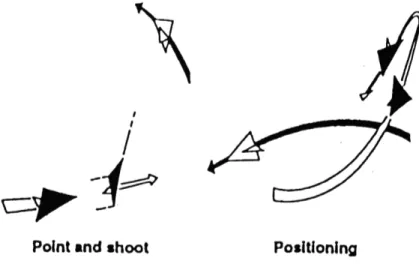
Wing rock is a concern for current and future aircraft because it proves to be a major maneuver limitation. The capability of modern combat aircraft to perform en-hanced agility maneuvers at high angles-of-attack, such as point-and-shoot maneuver and positioning (Figure 1-3), will suffer if wing rock comes into play, since it impairs the tracking and tactical effectiveness. In addition, it also poses a safety problem in some critical flight conditions, such as landing. In this situation, wing rock might cause loss of aircraft controllability and might prove to be catastrophic.

Because wing rock has potentially severe adverse effects on maneuver capability and safety, the alleviation or control of this undesirable motion is of great interest in the operation of modern aircraft. A good control strategy has to be devised in order to successfully alleviate the wing rock motion. The development of such strategy requires a thorough understanding of wing rock dynamics. Several work in the area as an attempt to gain a better understanding of wing rock motion has been reported, although none is comprehensive, especially in the multiple degrees-of-freedom cases. A brief review of the literature in the area will be presented next.

(12)

de -o (deg) (deg) Br (deg) lat stk (deg) (deg) a(deg (deg) ~*ii~

20J,

0

20

10 o.

-5 10 0 20.-10 0O

.

. L- 'r' ~ t " I : !0 i ,."

o

Figure 1-2: Wing rock motion as observed on the F-4 aircraft [4]

I

Point and shoot Positioning

Figure 1-3: Point-and-shoot and positioning maneuvers

(13)

1.2.1 Previous Work

While there is a considerable body of work on conventional flight dynamics, the situations involving nonautonomous or nonlinear flight regimes are infrequently in-vestigated. This is mainly because of the fundamental mathematical difficulties in dealing with such systems. Ramnath [30] analyzed the time-varying dynamics of a VTOL vehicle during a transition from hover to forward flight, by the Generalized Multiple Scales (GMS) method. Ramnath [34] also analyzed the re-entry dynamics of the space shuttle by the GMS method and developed a separation of the fast and slow aspects of the aircraft through variable flight conditions.

In particular, research on wing rock in the literature can be divided into three major groups. The division is based on whether the emphasis of the work is about the aerodynamic causes of wing rock, wing rock dynamics, or wing rock control.

On the subject of aerodynamic sources of wing rock, the most notably is the work done by Ericsson [12, 13, 14]. He investigates the fluid flow mechanisms causing wing rock. For aircraft with highly swept wing leading edges, wing rock is caused by asymmetric vortex shedding. For aircraft with straight or moderately swept leading edges, the causative mechanism of wing rock is usually the asymmetric airfoil stall. If the aircraft has a slender forebody, wing rock can also be generated by asymmetric body vortices from the nose. By representing the aerodynamic time history effect with a lumped time lag and by using the experimental static data, the amplitude of the wing rock can be predicted. However, in this method, the frequency of the wing rock must be known in advance for the amplitude prediction.

Several work emphasizing the dynamics of wing rock motion will now be described. A study of the aerodynamic factors which cause the low speed wing rock of a free-to-roll flat plate delta wing with 800 leading edge sweep is conducted by Nguyen et

al. [15]. Static force tests and dynamic wind tunnel experiments are utilized in their investigation. Their results indicate that the wing rock phenomenon is caused by a dependence of aerodynamic damping in roll on sideslip such that negative (unstable) roll damping is obtained at smaller sideslip angles and positive (stable) roll damping is obtained at the larger angles. A mathematical model of this effect is also developed and shown to agree closely with the experimental results.

Based on the test data in [15], Hsu and Lan [16] develop a mathematical model to calculate the wing rock characteristics. The amplitude and frequency of the wing rock motion are obtained analytically by solving the resulting dynamic equations using the Beecham-Titchener asymptotic method. They extend their analysis to also

(14)

include the case involving additional lateral degrees-of-freedom (sideslip and yaw). The result is a set of coupled nonlinear algebraic equations which can be solved through numerical iterations to get the amplitude and the frequency of the wing

rock.

In a series of papers [17-20], Nayfeh et al. present some numerical simulations and analytical study of wing rock phenomenon on slender delta wings. In the numerical simulation of free-to-roll delta wings in [17], the governing dynamic equation of rolling motion is coupled with the unsteady vortex-lattice method, which is then integrated using a predictor-corrector technique. The simulation and the experimental results are shown to be in agreement. Based on the numerical simulation results, some analytical models of single degree-of-freedom wing rock are developed and analysis of the models are done using Multiple Time Scales Method [18, 19]. In [20], the influence of the second degree-of-freedom in pitch on wing rock motion is simulated numerically. The results suggest that the motion of the two degree-of-freedom case can differ significantly compared to the single degree-of-freedom one. However, no analysis is given to explain the phenomenon.

Wing rock phenomenon on Gnat aircraft is considered by Ross [21]. Effects of cubic nonlinearities in roll rate and sideslip are considered and analytical approxi-mations of the solution using the Beecham-Titchener method were obtained. The analysis is performed by considering only the lateral degrees-of-freedom of the air-craft. As in [16], a set of nonlinear algebraic equations has to be solved numerically to get the amplitude and frequency of the resulting wing rock motion. It is shown that such nonlinearities can cause wing rock on the aircraft.

In [9, 10], Planeaux etal. examines the high angle-of-attack solution structure of an eight-state nonlinear equations of motion representative of a high performance fighter aircraft. A numerical approach using bifurcation theory and continuation method is used to trace the branches of both equilibria and periodic solutions. Their analysis shows that for some parameter combinations, wing rock can appear in the system. Since the focus of their work is mainly on obtaining the structure of the solutions at high angles-of-attack and on interpreting the results, no attempts are made to extract the parameters causing certain phenomena. In a similar fashion, Jahnke [11] performs a similar numerical analysis on various nonlinear aircraft equations of motion representing the F-15 aircraft. Wing rock is also shown to occur in the system for some parameter combinations.

Some work on wing rock control has also been reported. An example is the work of Luo and Lan [22], where the theoretical analysis of the optimal control input for wing

(15)

rock suppression is conducted. The one degree-of-freedom wing rock model in [16] is used in their analysis. Although the control law obtained in their analysis is quite complicated (a nonlinear function of roll angle and roll rate), after observing some simulations, they conclude that controlling roll rate is an effective way to suppress the wing rock. Other work involving the application of other nonlinear control methods, such as adaptive control and neural network, to the one degree-of-freedom model is given in [24, 25].

Most of the earlier work concerns wing rock on aircraft with only one degree-of-freedom in roll, although some attempts to extend the investigation to include more of-freedom have been made. Most of the work involving multiple degrees-of-freedom, however, is numerical in nature, hence the results apply only to specific cases considered.

1.3 Contributions of the Dissertation

This dissertation extends the previous work on wing rock in an attempt to gain a better understanding of the nonlinear aircraft dynamics. The extension includes the use of a more general nonlinear aircraft model in the analysis, the development of an analysis technique in the treatment of multiple rotational degrees-of-freedom wing rock cases, and the derivations of analytical solutions to the problem. The technique utilizes the powerful Multiple Time Scales (MTS) method in conjunction with the center manifold reduction principle and bifurcation theory. As we shall see later, this technique offers a systematic approach to uncover the important dynamics of the system and enables us to separate the rapid and slow aspects of the complex nonlinear dynamics. Moreover, the application of the above technique leads us to solutions in a parametric form, which enables us to see how each parameter influences the resulting system dynamics. The technique also leads to the development of a unified framework for the single and multiple degrees-of-freedom wing rock dynamics, the results of which can easily be utilized for control design.

The development of strategies for wing rock alleviation is also considered in the dissertation. The strategies are based on the results of the dynamics analysis. Unlike most of the previous work in the area, the control power issue is emphasized, as it is a main limiting factor for an aircraft flying at high angles-of-attack. Several control strategies are described and the advantages and disadvantages of each strategy are

(16)

1.4 Outline of the Dissertation

The discussion in this dissertation is arranged in the following order.

* Chapter 1 provides an introduction to the wing rock problem, discusses the previous work in the area, and describes the general contributions of the disser-tation.

* Chapter 2 describes in brief the theories and methods which are used in the analysis.

* Chapter 3 treats the simplest case of wing rock motion, where the aircraft is assumed to have only a single rotational degree-of-freedom in roll. This case is useful in building our understanding of the basic wing rock dynamics.

* Chapter 4 discusses the wing rock motion on an aircraft having two rotational degrees-of-freedom, in roll and pitch. It is shown that the additional degree-of-freedom increases the complexity of the analysis. Some interesting phenomena not found in the single degree-of-freedom case are noted and discussed.

* Chapter 5 considers an aircraft having the complete rotational degrees-of-freedom: roll, pitch, and yaw. A significant increase in the complexity of the analysis can be observed for this case as compared to the previous simpler cases. More interesting phenomena are also uncovered by the analysis.

* Chapter 6 describes the possible control strategies for the alleviation of wing rock motion. The effects of the limitation in controls are also discussed. Possible use of nonconventional control techniques to satisfy control power requirement to alleviate wing rock is also addressed.

* Chapter 7 provides the conclusions of the work described in the dissertation and also the recommendations for future work.

(17)

Chapter 2 Theories and Methods

2.1 Introduction

In the following sections, the main theories and methods directly used in the analysis of the wing rock problem are discussed. The interested reader may refer to the cited literature for a more detailed discussion of the subjects.

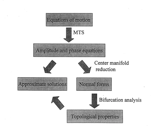
In general, the analysis is based on the Multiple Time Scales (MTS) method in conjunction with techniques derived from dynamical systems theory, such as Center Manifold Reduction techniques and bifurcation analysis. As we shall see later, these tools are very useful in uncovering the complex dynamics of the system.

2.2 The Multiple Time Scales Method

2.2.1 Concept

The concept of the Multiple Time Scales (MTS) Method described here is based on the work of Ramnath [27, 28, 29]. The interested reader may consult those references for a complete treatment of the method.

The motion of many dynamic systems consists of a mixture of fast and slow behaviors. Some parameters of a system may mainly affect the fast behavior, while some others may mainly affect the slow behavior of the system. In most dynamic systems, this is not easy to detect. Knowledge of how a certain parameter affects the system behavior would be very valuable, as this would provide a clue on what to

(18)

do if we are to alter the system behavior. For this reason, it would be advantageous to separate the fast and the slow behaviors of a system. The Multiple Time Scales

(MTS) approach is a technique based exactly on this idea.

The MTS method belongs to a larger body of knowledge called Perturbation Meth-ods. As with other perturbation methods, the MTS method enables us to obtain approximate solutions to a problem in limiting cases. This kind of problem is usually recognized by the existence of a very small or very large parameter in a system. In dynamic systems the existence of such parameters generally implies the existence of fast or slow behaviors. Since many physical systems of interest contain such parame-ters, the MTS method can find a wide range of applications. One example of such a system is a rigid body in orbit around the earth (see [31]). For this system, the small parameter is the ratio of the orbital frequency to the nutational frequency.

The main concept of the MTS approach is selecting the appropriate scales to observe the behavior of a system. For a dynamic system, in most cases time is the independent variable, hence the words time scales or clocks are often used instead of scales. In general, one can employ as many scales as one wishes to represent the dynamics of a system, depending on the level of accuracy to be achieved. In many applications, however, the use of only two scales is adequate to capture the important dynamics of the system. It is worth noting that the choice of scales determines the quality of the solution. The inappropriateness of the scales used will show up as an incompatibility with the assumptions previously made or as a nonuniformity in the solution.

The time scales used in the MTS method are generally real and linear. Ram-nath [27, 29] generalized the method to the Generalized Multiple Scales (GMS) method by including nonlinear and complex scales. In general, the GMS method intro-duces additional degrees-of-freedom to the problem, which can be used to determine the appropriate time scales for the problem. Because of this reason, this approach nor-mally generates better results than the regular MTS approach. Several applications of the GMS method in science and engineering can be found in [29, 33, 34, 35].

2.2.2 Mathematical Concept of the MTS Approach

The following is based on the development of Ramnath and Sandri [27]. The MTS approach relies on the concept of extension. The fundamental idea of the concept of extension is to enlarge the domain of the independent variable to a space of higher dimension. Since our main interest is on dynamic systems, we will think of time as

(19)

T2

very slow motions

extension / slow motions t mixed behavior to fast motions

Figure 2-1: The concept of extension

our independent variable. Time as the independent variable is extended to a set of new independent timelike-variables which are called time scales or clocks. Each clock captures a certain behavior of the system. For example, the fast clock captures only the fast behavior of the system. The extension of time t is symbolized as follows :

t -- + T7, 71,. .,Tn} (2.1)

where ro, T1, . ., 7, are the time scales or the clocks, which are normally functions of

t and the small or large parameter in the system E, that is

Ti = ti(t, E) (2.2)

How -i relates to t determine the nature of the time scale. In GMS approach, this relation is determined in the course of analysis and not determined a priori. The relation of T- to E in this case determines whether the clock is fast or slow. Figure 2-1 shows a schematic illustration of the concept.

Suppose now that y(t, 6) is the dependent variable in a dynamic equation and restrict the discussion to a dynamic equation in the form of an ordinary differential equation. Then, since t is extended, y(t, e) is also extended as

y(t, E) -+ Y(0, '1, -... n; 6) (2.3)

It is understood from the discussion above that due to the extension of the inde-pendent variable, an ordinary differential equation will become a partial differential equation. This is not a limitation, however, since the resulting partial differential

(20)

equation is usually simpler than the initial ordinary differential equation.

From the definition of extension, when Equation (2.2) is inserted into extended function Y we have

Y(ro(t, E),Ti (t,E),...,r(t, E); E) = y(t, 6) (2.4) The result of substituting the trajectory in the extended function Y is called the restriction of Y.

2.2.3 Principle of Minimal and Subminimal Simplification

The following treatment is based on the development by Ramnath [32]. The purpose of all approximation methods, including the MTS method, is to make a difficult problem become more tractable. In essence, by employing these methods, one wishes to have a simpler problem. One subtle question is; how far can one simplify a problem. Of course, what one wants is to capture all the important behaviors of the system. In other words, the simplification should be as minimal as possible so as to retain all the important information of the system. This is called the principle of minimal

simplification. This facilitates a derivation of the correct and optimal ordering of the terms in the mathematical model which then leads to accurate asymptotic solutions in a systematic manner.

There are some cases where the principle of minimal simplification needs to be extended in order to develop meaningful solutions. This refinement, i.e. the principle

of subminimal simplification was developed by Ramnath [27, 33] and has been applied succesfully in several cases (see [33] and [35]).

2.3 Dynamical Systems Theory

Some main points of dynamical systems theory that are used in the later analysis are discussed briefly in the following subsections. The interested reader may refer to the literature [36, 38, 39] for a more detailed development of the subjects.

A dynamical system is a set of ordinary differential equations of the form

(21)

where x E R1, f is an n-dimensional vector field, t is time, and u E Rm. (-) represents differentiation of (.) with respect to time t. n is referred to as the dimension of the system. The representation (2.5) shows explicit dependence on time, t. A dynamical system with this property is called nonautonomous.

Many physical systems can be represented by dynamical systems, including air-craft equations of motion. Although in general, the airair-craft motion is nonautonomous, work in this dissertation will be focused on the situations where the aircraft equations of motion can be validly assumed to be time independent. Dynamical systems of this type are called autonomous and have the form

ic = f(x; y) (2.6)

The discussion in the next subsections is limited to the autonomous type of system. Another assumption made in the following discussion is that all vector fields con-sidered are smooth. This means that the vector field and all of its derivatives are continuous. This assumption allows us to ignore the questions about the degree of differentiability of the vector field for the theorems introduced in the subsequent subsections.

The solution history of a dynamical system for some initial condition is usually referred to as a trajectory. The solution trajectories are smooth for smooth vector fields. For many systems, including aircraft, it is impossible to determine the solution trajectories exactly. Therefore, some approximation techniques have to be employed to find the approximation of the solutions.

The families of solution trajectories of a system can be expressed graphically in the phase space, that is the Euclidean space of the dependent variables. The shortcoming of phase space representations is that for systems of dimension four or higher, it is not possible to show the entire phase space in one plot. In this situation, the phase space has to be projected onto two or three dimensional space, and this makes the interpretation of the system behavior more difficult. For low dimensional systems, phase space representations can be very useful and can provide clear pictures of the system behavior.

2.3.1 Equilibrium Points and Their Stability

Equilibrium points or fixed points are points in phase space where all time deriva-tives are zero. As its name implies, these points describe the equilibrium states of

(22)

the system but provide no information about the transient response of the system. Equilibrium points of the system (2.6) are determined by solving the equation

f(x; /) = 0 (2.7)

It is equivalent to finding the zeros of a set of algebraic equations, which are in general nonlinear. In many problems, finding zeros may not be an easy task, however there have been many techniques developed to overcome this difficulty (for example, see [40]). Note also that one can always apply a transformation to (2.7) such that it has an equilibrium point at the origin. Such an equilibrium point is also referred to as zero solution. Often in a physical system, the zero solution represents the nominal or equilibrium condition of interest.

The stability of an equilibrium point provides an important information in a dy-namical system. It determines whether the states of the system are attracted or repelled from the equilibrium point. In general, one can differentiate two types of stability : global stability and local stability. Global stability characterizes the stabil-ity of an equilibrium point for any initial condition in the phase space, while local stability determines the stability of an equilibrium point in a small region around the point. Global stability information, while useful, is very difficult to obtain in most situations. Fortunately, in many cases, local stability information, which is easier to obtain, is enough to uncover the important dynamics of a system.

The local stability of an equilibrium point of a nonlinear dynamical system can be derived using the Poincare-Liapunov's linearization method. The great value of this method lies in the fact that under certain conditions, the local stability properties of a nonlinear system can be inferred by studying the behavior of a linear system, which is obtained by linearizing the nonlinear system around an equilibrium point of interest. Then the stability can be determined by calculating the eigenvalues of the linearized system. An equilibrium point is asymptotically stable if the real parts of all eigenvalues are negative and unstable if any eigenvalue has a positive real part. If one or more eigenvalues have zero real parts, then the stability of the nonlinear system cannot be deduced from the linearized system. In this case, one has to use other means to determine stability, such as the Center Manifold theorem, which will be discussed in the next subsection.

The linearization of the system (2.6) at an equilibrium point (x*; p*) is

(23)

where u = x - x* and Vf(x*; p*) is the Jacobian matrix of f evaluated at (x*; t*), or

symbolically

Vf(x*; p*)= x= ,= (2.9)

The eigenvalues of Vf(x*; /*) determine the stability of the equilibrium point (x*; t*) as discussed in the above.

2.3.2 Center Manifold Theory

An invariant manifold of a dynamical system is a curve in phase space such that a solution trajectory starting from a point on that curve will remain on the curve for all time. Based on this definition, any equilibrium point is also an invariant manifold because if a system starts at an equilibrium point, it will stay there forever. We will specifically look at the invariant manifolds of an equilibrium point, that is the invariant manifolds that contain the equilibrium point. The stable manifold of an equilibrium point is an invariant manifold containing the equilibrium point such that if the system starts on the invariant manifold, it will asymptotically approach the equilibrium point as time goes to infinity. The unstable manifold can be defined in the same manner, only reversely, that is the system starting on the invariant manifold will asymptotically approach the equilibrium point as time goes to negative infinity. Mathematically, these can be expressed as

WS = {x-+x*ast-+oo}

WU = {x-x*ast-+ -oo} (2.10)

where Ws and Wu symbolized the stable and unstable manifolds respectively. For a linear system, such manifolds are called stable and unstable eigenspaces and defined respectively as follows

E" = span{vilJ(Ai) < 0}

E" = span{vilJ(Ai) > 0} (2.11) where vi is the eigenvector and Ai is the corresponding eigenvalue. The notation R(-) denotes the real part of the term in the parenthesis. We note without proof that W s and Wu of a nonlinear system are tangent to ES and Eu of the corresponding linearized system [38]. This makes sense intuitively as the behavior of a nonlinear system in the neighborhood of an equilibrium point can be approximated by the

(24)

Es

EC

Figure 2-2: Illustration of stable, unstable and ceriter manifolds

behavior of the linearized system about the equilibrium point in the absence of pure imaginary eigenvalues (zero real part).

In the case where eigenvalues with zero real part are present, one can define center eigenspace as follows

EC = span{vij(Ai) = 0} (2.12)

In a way similar to the stable and unstable manifolds, a center manifold (Wc can also be defined for a nonlinear system. The center manifold of an equilibrium point is an invariant manifold that contains the equilibrium point and is tangent to the center eigenspace of the linearized system. Note that no evolution information is given by the definition. This is because one cannot draw conclusions about the behavior of the nonlinear system around an equilibrium point from the corresponding linearized system having a center eigenspace. The behavior of the system on the center manifold has to be examined in the nonlinear context. An illustration of the nonlinear and linear manifolds is given in Figure 2-2. Several theorems on center manifolds which will be useful for later analysis are discussed next.

We consider the system of the following form ic = Ax + p (x,y)

Sr = By + q(x,y) (2.13)

where x E R', y E Rm, A and B are constant matrices such that R(Ai[A]) = 0 ; i =

1,...,l and R(Ai[B]) < 0 ; i = 1,...,m. The functions p and q along with their Jacobians vanish at the origin, which is the equilibrium point of interest. In other words, p(O, 0) = V(0, 0) = 0 and q(0, 0) = Vq(0, 0) = 0.

(25)

The linearized equation around the origin in this case takes the form i = Ax

y = By (2.14)

This system has two obvious eigenspaces, namely x = 0 and y = 0 which represent stable and center eigenspaces, respectively. As t -+ oo all solutions of Equation (2.14) tend to go exponentially to the solutions of

i = Ax (2.15)

That is, the equation on the center eigenspace determines the asymptotic the solutions of the system (2.14) modulo exponentially decaying terms. results can be expected for the nonlinear system.

behavior of Analogous

First, it is a well-known result that the system (2.13) possesses a center manifold, as stated in the following theorem.

Theorem 1 [39] Equation (2.13) has a local center manifold y = h(x) for Ixi < 6, 0 < 6 < 1, where h(0) = Vh(0) = 0

The flow on the center manifold is then governed by the i-dimensional system

i

= Az + p(z, h(z)) (2.16)

which generalizes the corresponding problem (2.15) for the linearized case. The con-ditions h(0) = Vh(O) = 0 reflect the tangency of the center manifold to the center eigenspace at the origin. The dynamics of the system will converge to the dynamics of the center manifold after some transients as stated in the following lemma.

Lemma 1 [39] Let (x(t),y(t)) be a solution of Equation (2.13) with I(x(0),y(0))l sufficiently small. Then there exist positive constants K and v such that

ly(t) - h(x(t))I < K exp (-vt) y(O) - h(x(0)) I (2.17) for all t > 0.

Therefore it can be understood that information to determine the asymptotic as stated in the following theorem.

Equation (2.16) contains all the necessary behavior of the solutions of Equation (2.13),

(26)

Theorem 2 [39] (a) The zero solution of Equation (2.16) has the same stability prop-erty as the zero solution of Equation (2.13).

(b) Suppose the zero solution of Equation (2.16) is stable. Let (x(t), y(t)) be a solution of Equation (2.13) with (x(O), y(O)) sufficiently small. Then there exists a solution z(t) of Equation (2.16) such that as t --+ o0

x(t) = z(t) + O(exp (-t))

y(t) = h(z(t)) + O(exp (-yt)) (2.18) where 7 > 0 is a constant depending only on B.

This result enables one to deal only with an 1-dimensional equation, which is the dimension of the center manifold, to obtain the asymptotic behavior of the (1 + m)-dimensional system. This systematic order reduction method is called center manifold

reduction.

Now we will discuss on how to compute the center manifold. The substitution of

y = h(x) into the second equation in (2.13) and the use of chain rule yield

Vh(X) [Ax + p(x, h(x))] = Bh(x) + q(x, h(x)) (2.19) or

N(h(x)) _ Vh(X) [Ax + p(x, h(x))] - Bh(x) - q(x, h(x)) = 0 (2.20) This equation together with the conditions h(O) = Vh(O) = 0 is the system to be solved for finding the center manifold. Unfortunately, this equation for h(x) in general cannot be solved exactly, since to do so would imply that a solution of the original equation had been found. The next theorem, however, shows that in principle, its solution can be approximated arbitrarily closely.

Theorem 3 [39] If a function O(x), with t(0) = Vo(O) = 0, can be found such that

N(t9(x)) = O(x'r) for some r > 1 as Ix| -- 0 then it follows that as x - 0,

h(x) = 9(x) + O(|xlr) (2.21)

In case the center manifold is analytic, we can approximate h(x) to any degree of accuracy by seeking series solutions of (2.19).

(27)

2.3.3 Bifurcation Analysis

The term bifurcation was originally used to describe the branching of equilibrium solutions in a family of differential equations as certain parameters are varied. Bifur-cations of equilibria are normally accompanied by changes in the topological prop-erties of the solutions. For system (2.5), p = po is called a bifurcation point if the qualitative nature of the solutions of (2.5) changes at p = Po. That means that in

any neighborhood of p = po, there exist P1 and P2 such that the topological behavior of the solutions of (2.5) for p = 1 and P = P2 are not equivalent.

In this section, only one parameter bifurcation (also called codimension one bi-furcation) is discussed. Such bifurcation normally occurs in one or two dimensional systems. As we shall see, although the dimension of the aircraft equations of mo-tion in general is greater than two, the applicamo-tion of the center manifold technique described above could reduce the representation of the important dynamics of the system into one or two dimensional equations. The bifurcation analysis can then be done on this reduced system. Several prototypical one parameter bifurcations are discussed next.

Consider the first order system

S= ~ + 2 _{- f(x)} _(2.22)

where p is a parameter, which maybe positive, negative, or zero. The Jacobian of the system in this case is

Vf(x) = 2x (2.23)

When p is negative, there are two equilibrium points at x* = + -J with Vf(x*) = ±2 _i pj. The linearized system around each of the equilibrium points is

it = Vf(x*)u (2.24)

Here, the Jacobian is the same as the eigenvalue of the linearized system. Based on the stability theory discussed earlier, the equilibrium point at x* = - FI is stable and the one at x* =

I

_{is unstable (see Figure 2-3). As p approaches zero from below,} the parabola moves up and the two equilibrium points move toward each other. When p = 0, the two equilibrium points coalesce into the so-called half-stable equilibrium point at x* = 0 (see Figure 2-3). Such an equlibrium point is very delicate, it vanishes as soon as p moves away from zero. There are no equilibrium points when p > 0 (see Figure 2-3). In this example, p = 0 is the bifurcation point of the system, since the

(28)

(b) =0 (c) >0

Figure 2-3: The plots of k = p + x2 _{as p varies}

unstable - X

stable

Figure 2-4: The bifurcation diagram of = p + x2

system is qualitatively different for p < 0 and for M > 0.

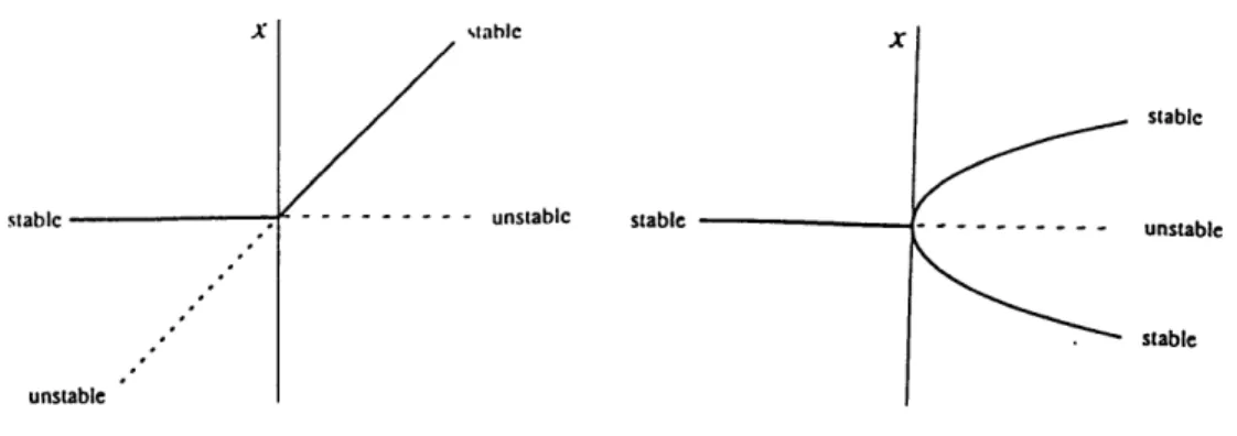
Bifurcation is often represented in a diagram the showing the values of the equi-librium points and their stability as a parameter varies. Such diagram is called a bifurcation diagram. The bifurcation diagram for the example above is given in Fig-ure 2-4. In the diagram, the solid line indicates the locus of the stable equilibrium points, while the dotted line indicates the locus of the unstable equilibrium points. Bifurcation of this type is called saddle-node bifurcation.

Other types of bifurcation, which typically occur in a one dimensional system, are transcritical and pitch fork bifurcations. The prototypical first order equations for the occurence of these types of bifurcation and their bifurcation diagrams are shown in Figure 2-5. The transcritical bifurcation is characterized by the exchange of stabilities between the equilibrium points. In the example, the two equilibrium points do not dissappear after the bifurcation (as in the saddle-node case), they merely switch their stability. Pitchfork bifurcation is common in physical problems that have a symmetry, where the equilibrium points tend to appear and dissappear in symmetrical pairs.

(29)

X ltbihlc

stable

stabic unstablec stable -- unstable

stable

unstable

Figure 2-5: Transcritical and pitchfork bifurcations

The term 'pitchfork' becomes clear from the shape of the bifurcation diagram for this type of bifurcation. There are two different types of pitchfork bifurcation and they are categorized as supercritical and subcritical (see Figure 2-5). Note that in the subcritical case, the only stable equilibrium is x* = 0 when p < 0.

In systems of dimension two or greater, more than one eigenvalue could be zero at the bifurcation point and this gives rise to a very involved situation. Such a sit-uation, however, occurs very rarely, and hence it will not be discussed further here. A more important case occurs when the system posseses a pair of pure imaginary eigenvalues at certain parameter value. In this situation, if the stability type of the equilibrium changes when subjected to perturbations, then this change is usually ac-companied with either the appearance or dissappearance of a periodic orbit encircling the equilibrium point. This type of bifurcation is called Hopf bifurcation and is of-ten encountered in physical systems. The following theorem formulates this type of bifurcation formally.

Theorem 4 [37, 38] Let 5 = f(x, p) be a dynamical system of dimension two de-pending on a scalar parameter M with f(0, p) = 0. Assume that the linearized

system at the origin ii = Vf(0, p) has the complex conjugate eigenvalues A(A)

with R(A(0)) = 0 and Q(A(O)) : 0. Furthermore, suppose that the eigenvalues cross the imaginary axis with nonzero speed, that is

d _{(0) :A 0}

(2.25)

Then, in any neighborhood N of the origin and any given /to > 0 there is a

p

with I

p

< 0Lo such that the differential equation x = f(x, p) has a nontrivial periodic orbit in N.

(30)

MTS

SON

Center manifold

reduction

Bifurcation analysis

Figure 2-6: The analysis technique utilizing the MTS method, center manifold reduc-tion principle, and bifurcareduc-tion theory

It is interesting to note that the above theorem allows us to detect the occurence of a periodic orbit in a nonlinear system by examining the properties of the eigenvalues of the corresponding linearized system. However, to learn more about the properties of the resulting periodic orbit, such as its stability, one has to do further analysis by including the nonlinear terms.

2.4 Methodology

By virtue of the methods discussed so far, Figure 2-6 shows schematically the logical flow of their application in the analysis.

(31)

a small parameter, e, the MTS method is then applied. The time scales used in the analysis are selected based on the Principle of Minimal Simplification and its extensions. As we shall see later, the systems of interest are oscillatory in nature and the application of the MTS method usually leads to the amplitude and phase-correction equations in the slower time scales. These equations may or may not be solvable, depending on the system. In the single degree-of-freedom wing rock case, the amplitude and phase-correction equations are solvable analytically. However, in the multiple degrees-of-freedom cases, these equations are coupled and hence are very difficult to be solved exactly. As we can see later, in all cases we consider in the dissertation, the amplitude equations can be solved independently from the phase-correction equations. The phase-phase-correction equations can usually be solved once the solution of the amplitude equations are found. This fact simplifies the problems. However, it should be remembered that in the multiple degrees-of-freedom cases, the amplitude equations are also multi dimensional and coupled.

As we have mentioned, the exact solutions of the amplitude equations are very difficult or may be imposible to obtain. Approximate solutions can be derived with some information of the system dynamics, such as its topological properties. To obtain such properties, we first simplify the problem by reducing its dimension using the center manifold reduction principle. Bifurcation analysis can then be performed on the reduced dimensional system to get the topological picture of the system around the equilibrium point of interest. As we can see from Figure 2-6, the information on the topological properties of the system will be used to obtain the analytical approximation of the solution.

The above paragraphs describe the technique of analysis in general. The tech-nique provides a systematic approach to obtain approximate solutions to the prob-lems. Moreover, the application of the technique leads to considerable insight into the complex phenomenon, as will be demonstrated in the next three chapters.

(32)

Chapter 3 Single Degree-of-Freedom Wing

Rock

3.1 Introduction

In this chapter, a simplified treatment of the problem is considered, where it is as-sumed that the aircraft has only one rotational degree-of-freedom in roll. This simpli-fication is based on the fact that the wing rock motion in most situations is dominated by oscillations in roll. Most published work on wing rock deals with such simplified case [12-18]. The largely available data of wind tunnel experiment on wing rock mo-tion for a one degree-of-freedom aircraft or wing model also explains why much work is focused on this very special case.

Although relatively less difficult, a great deal of insight can be gained by study-ing the sstudy-ingle degree-of-freedom wstudy-ing rock problem. Note however, that because of the model limitation, some important physical effects, such as aerodynamic cross-coupling, are not included.

This chapter revisits and extends the previous work on single degree-of-freedom wing rock dynamics. It serves as a basis for later work on multiple degrees-of-freedom cases, which require more complex analysis.

(33)

Figure 3-1: The aircraft axis systems"

3.2 Equation of Motion

In this and subsequent chapters, the Lagrangian approach is used in deriving the equations of motion of the aircraft. This approach reduces the formulation of prob-lems in dynamics to that of the variation of a scalar integral irrespective of the coordinate systems used. Note that for the simple case of single rotational degree-of-freedom motion, the equation of motion can be derived easily using any available methods. However, the Lagrangian approach will be used in this derivation to pro-vide uniformity with the derivations in subsequent chapters, which deal with multiple degrees-of-freedom- problems.

The axis systems needed in deriving the equations of motion are established next. The first axis system is denoted as XoYoZo and referred to as the stability axis system. Its origin is at the center of mass of the aircraft and the orientation of the axes describes the nominal or unperturbed attitude of the aircraft. The Xo axis is oriented towards the nominal nose direction of the aircraft, the Zo axis is on the nominal vertical plane of the aircraft pointing down and perperdicular to the Xo axis, while the Y axis completes the righthanded axis system. The second axis system (XbYbZb) is called the body-fixed axis system. As the name implies, this axis system has its

origin on the center of mass of the aircraft and it is fixed to the aircraft body. The Xb axis points towards the nose of the aircraft, the Zb axis is on the aircraft vertical plane and perpendicular to Xb, while Yb completes the righthanded axis system. In nominal flight condition, these two axis systems coincide with each other. See Figure 3-1.

(34)

degree-of-freedom in roll. Hence, in this case, Xb and Xo axes coincide. Perturbations in the system will only make the aircraft rotate about this axis. In perturbed situation, the Y axis of the body and stability axis systems makes an angle

4

with respect to each other. Similarly for the Z axis. This angle is called roll angle. Because of the assumption, the angular rate of the aircraft can simply be expressed as follows.

w = P Ixb

= ¢ixo (3.1)

where the notation i denotes the unity vector along the axis described in its subscript. Following the usual convention, p denotes the roll rate of the aircraft. For this special case, p = q.

As the aircraft has only the degree-of-freedom to roll, the rotational kinetic energy of the aircraft is given by

T = -1xx2 _(3.2)

where I~, is the moment of inertia of the aircraft about the Xb-axis. By substituting the above expression of kinetic energy into the Lagrange's equation

d--= - T Q

(3.3)

we get

i¢x = Q (3.4)

where Q is the generalized force, which is assumed to be contributed solely by the aerodynamics. The generalized force in this case is just the aerodynamic rolling moment of the aircraft. The generalized force, Q, can be found using

6W

Q

= (3.5)

which is basically the variation of the work done by the generalized forces due to the variation of the generalized displacement. The influences of gravity and propulsive forces are neglected in current analysis. Also, since we are interested in the free motion of the aircraft, we assume that no controls have been applied to the aircraft system. We will now discuss the aerodynamic moment acting on the aircraft.

(35)

3.3 Aerodynamic Moment

In this section, the aerodynamic moment on the aircraft is derived. The purpose of this section is to find the appropriate nonlinear form of aerodynamic moment to be used in the analysis. The details of the aerodynamic coefficients appearing in the final moment expression are of no importance at this point. These coefficients can be calculated by interpolating a polynomial of a certain order to the aerodynamics data of the aircraft found by using various techniques : analytical, computational, or experimental. This point will be further clarified as we proceed with the derivation.

The aerodynamic moment is derived under the assumption that the air flow around the aircraft is incompressible and quasi-steady. Simple modified strip theory aero-dynamics is utilized in the derivation, since, as we have stated before, we only need to obtain an appropriate expression of the aerodynamic moment. In the usual strip theory, the local aerodynamic force is determined solely by the aerodynamic proper-ties of each aircraft segment (CL vs. a, CD VS. a) and the gross angle-of-attack of the aircraft, with no consideration of three dimensional flow effects. Here, to keep the generality of the aerodynamic moment developed, the three-dimensional effect of the flow is taken into account. Because of this effect, each segment of the aircraft may see a different effective angle-of-attack. Nominally, it is assumed that the aircraft flies a horizontal straight path at specific angle-of-attack. It is also assumed that only the wings and the horizontal tail of the aircraft are effective in generating the aerodynamic forces.

We consider the derivation of aerodynamic forces on the wing in detail. The derivation for the horizontal tail will then follow in a similar fashion. Consider a streamwise segment of the wing of width dy. The incremental lift and drag forces produced by this segment are

dL(y) = qc(y)cL(y)dy

dD(y) = qc(y)cD(y)dy (3.6)

where q = 1pV2 _{is the dynamic pressure, c(y) is the airfoil chord at location y along}

the Yb axis, CL(y) and cD(y) are the local lift and drag coefficients, respectively. The relationship of the local lift and drag coefficients (cL(y) and cD(y)) on the local effective angle-of-attack (ae(y)) is represented by a cubic polynomial as follows.

2 3

CL = CLo + CLLi e + CL2ae + CLa e

2 3 _(3.7)

(36)

As we will point out later, the inclusion of the cubic terms in the above relations is necessary for the generation of wing rock motion. In Equation (3.7), the dependence of the coefficients and a on the spanwise location, y, has been omitted for simplicity.

The effective angle-of-attack distribution along the wing span consists of several contributions. For the one degree-of-freedom case, in general, this distribution de-pends on the nominal angle-of-attack, roll rate, sideslip angle and sideslip rate. Since we only consider small deviations from the nominal condition, then the contributions of the above factors on the effective angle-of-attack distribution can be expressed using a linear relation as follows.

ae(() = al(y) +

p+

+

.

(3.8)

Op i 3+

or alternatively,

ae (Y) = 1(Y) + 2 (Y) + 3 (Y) + 04 (Y) (3.9) where al(y), a2(y), O3(Y), _{and 0a4(Y) indicate the component of the effective} attack distribution contributed by the nominal angle-attack, roll rate, angle-of-sideslip, and sideslip rate, respectively. The following itemization describes each of the above components briefly.

* Nominal angle-of-attack (ao).

Since the aircraft in the nominal condition is assumed to fly symmetrically, then the resulting effective angle-of-attack distribution due to ao is symmetric. This distribution generates aerodynamic forces necessary to keep the aircraft in equilibrium. For a wing in three dimensional flow,

) = a(y) - a,(Y) (3.10)

where ae(y) denotes the local true angle-of-attack seen by the local wing section,

ag denotes the local angle-of-attack in case the flow is two dimensional, and ai(y) denotes the induced angle-of-attack, which is basically a three-dimensional effect. Equation (3.10) can be expressed as

a, (y) = sin-'(sin ao cos r cos ) - ai(y) (3.11)

where F is the dihedral angle of the wing. * Roll rate (p).

(37)

the left wing tip up. It is clear therefore that positive roll rate increases the effective angle-of-attack seen by the right wing and decreases the one seen by the left wing. In this work, it is assumed that the angle-of-attack distribution due to roll rate is perfectly antisymmetric and can be generally expressed using

a2() = f2(y)P (3.12)

where f2(Y) is an odd function of y, which may take into account the three dimensional nature of the flow. In a simple case where the three-dimensional aerodynamic effects are absent, a2 is given by

2M(y) = (3.13)

where U is the component of the aircraft speed on the Xb-axis. * Angle-of-sideslip (0).

Nonzero angle-of-sideslip indicates the presence of cross flow, and such a cross flow destroys the symmetry of the flow and induces changes in the angle-of-attack seen by each streamwise segment of the wing. For an aircraft flying at high angles-of-attack, the angle-of-sideslip can be induced by the deviation of the aircraft from the wing level position. At low angles-of-attack, the induced angle-of-sidelip is negligible. The magnitude of the incremental angle-of-attack due to sideslip is dependent on several factors such as wing dihedral angle, wing position on the fuselage (high, low or mid), fuselage shape and wing sweep angle. The angle-of-attack distribution generated by this effect is assumed to be antisymmetric and can be expressed as

Co3(y) = f3(y) (3.14) f3(y) is an odd function of y, whose values and sign depend on the factors mentioned above.

* Sideslip rate ()

The f effect is mostly due to the lag effect of the flow between the right and left wings. The component of the effective angle-of-attack distribution due to this effect is assumed to be antisymmetric and is expressed as

a4(Y) = f4(y) (3.15)

Aircraft wing rock dynamics and control

Aircraft Wing Rock Dynamics And Control

Tiauw Hiong Go

@

DEC 2 8 1999

Aircraft Wing Rock Dynamics And Control

by

Tiauw Hiong Go

Abstract

dedicated to

Jusvin and Jason

who have been my inspiration

Simplicity is the glory of expression

Acknowledgments

Contents

Chapter 1

Introduction

1.1

Background

1.2

Wing Rock Phenomenon

20J,

20

10

o.

.

o

I

1.2.1

Previous Work

1.3

Contributions of the Dissertation

1.4

Outline of the Dissertation

Chapter 2

Theories and Methods

2.1

Introduction

2.2

The Multiple Time Scales Method

2.2.2

Mathematical Concept of the MTS Approach

2.2.3

Principle of Minimal and Subminimal Simplification

2.3

Dynamical Systems Theory

2.3.1

Equilibrium Points and Their Stability

2.3.2

Center Manifold Theory

i

2.3.3

Bifurcation Analysis

I

p

p

MTS

SON

Center manifold

reduction

Bifurcation analysis

2.4

Methodology

Chapter 3

Single Degree-of-Freedom Wing

Rock

3.1

Introduction

3.2

Equation of Motion

4

Q

3.3

Aerodynamic Moment

ae(() = al(y) +

p+

+

.

(3.8)