Possible Deep Structure and Composition of Venus with Respect to the Current Knowledge from Geodetic Data

HAL Id: hal-03266988

https://hal.archives-ouvertes.fr/hal-03266988

HAL is a multi-disciplinary open access archive for the deposit and dissemination of sci-entific research documents, whether they are pub-lished or not. The documents may come from teaching and research institutions in France or abroad, or from public or private research centers.

L’archive ouverte pluridisciplinaire HAL, est destinée au dépôt et à la diffusion de documents scientifiques de niveau recherche, publiés ou non, émanant des établissements d’enseignement et de recherche français ou étrangers, des laboratoires publics ou privés.

Possible Deep Structure and Composition of Venus with

Respect to the Current Knowledge from Geodetic Data

Chi Xiao, Fei Li, Jianguo Yan, Michel Grégoire, Weifeng Hao, Yuji Harada,

Mao Ye, Jean-pierre Barriot

To cite this version:

Chi Xiao, Fei Li, Jianguo Yan, Michel Grégoire, Weifeng Hao, et al.. Possible Deep Structure and Composition of Venus with Respect to the Current Knowledge from Geodetic Data. Journal of Geo-physical Research. Planets, Wiley-Blackwell, In press, �10.1029/2019JE006243�. �hal-03266988�

Possible Deep Structure and Composition of Venus with Respect to

the Current Knowledge from Geodetic Data

Chi Xiao1,2_{, Fei Li}1,3_{, Jianguo Yan}3_{, Michel Gregoire}4_{, Weifeng Hao}1_{, Yuji Harada}5_, Mao Ye3_{, Jean-Pierre Barriot}3,6

1_{Chinese Antarctic Center of Surveying and Mapping, Wuhan University, Wuhan 430079, China} 2_{Laboratory of Earthquake Geodesy, Institute of Seismology, China Earthquake Administration,}

Wuhan 430071, China

3_{State Key Laboratory of Information Engineering in Surveying, Mapping and Remote Sensing,}

Wuhan University, Wuhan 430079, China

4_{Géosciences Environnement Toulouse, Observatoire Midi-Pyrénées Université Paul Sabatier}

Toulouse III-CNRS-CNES-IRD, Toulouse, France

5_{Space Science Institute, Macau University of Science and Technology, Avenida Wailong, Taipa,}

Macau, China

6_{Geodesy Observatory of Tahiti, BP 6570, 98702 Faa’a, Tahiti, French Polynesia}

Corresponding authors: Fei Li (fli@whu.edu.cn) and Jianguo Yan (jgyan@whu.edu.cn).

Key Points

 Our results show that the existence of Venus’s inner core cannot be constrained by the present-day observed tidal Love number k2.





Accepted

Article

This article has been accepted for publication and undergone full peer review but has not been through the copyediting, typesetting, pagination and proofreading process, which may lead to differences between this version and the Version of Record. Please cite this article as doi: 10.1029/2019JE006243.

Accepted

Article

Abstract

Almost no in situ seismic data are available for Venus; therefore, we can constrain the deep structure of this planet only from the geodetic data obtained by spacecraft. Of particular interest is Venus’s core-mantle boundary, which holds clues about the origin and evolution of this celestial body. In this study, we build a series of different mantle/core models of Venus based on several mantle composition models and compare their associated Love numbers k2 with the observed values. Due to the large uncertainty in the observed values of k2, the state of Venus’s core cannot be reliably constrained. However, the expected precision of k2 obtained by the EnVision mission will sufficiently reduce the acceptable model space and contribute to estimating the mantle viscosity structure. Based on current geodetic data, we find that the bottom of Venus’s mantle may not feature a phase transition from perovskite to post-perovskite if the FeO content of the mantle is less than 8.1 wt%; this region may be different from Earth’s D” layer. Furthermore, we find that the combination of observed k2 and Q can be used to distinguish whether the lowermost part of Venus’s mantle is a high-temperature basalt layer or a thin thermal boundary layer if observations of Q can be obtained.

Plain Language Summary

The deep structures of Venus and Earth may be different. However, due to the lack of seismic data, we need to use data obtained by orbital spacecraft. We can constrain the deep structure of Venus using tidal parameters that characterize tidal deformation, as these parameters are sensitive to the mantle viscosity, temperature profile, and core radius. By using forward modeling, we present evidence from observed tidal parameters that the bottom of Venus’s mantle may not feature a phase transition from perovskite to post-perovskite if the iron content of Venus’s mantle is no more than that of Earth’s mantle (~8.1% FeO). We also quantify how future observations of tidal parameters will improve our understanding of Venus’s mantle viscosity.

Accepted

Article

1. Introduction

Venus was once considered to be the sister planet of Earth because of the similarities between their masses and radii. Therefore, researchers initially believed that Venus has an internal structure similar to that of Earth. However, the first space mission to Venus revealed tremendous differences between the surfaces of the two planets. Venera 9 was the first lander to return images from the surface of Venus; the mission also collected data about the surface pressure, temperature, wind velocity and material composition (Florensky et al., 1977), changing our understanding of the planet. We now know that there are significant differences between the surfaces of Earth and Venus. Carbon dioxide dominates the atmosphere of Venus (composing approximately 96%), and the atmospheric pressure at the surface is approximately 9.2 MPa with a surface temperature near 730 K (Taylor, 1985). Moreover, Venus lacks plate tectonics (Spohn et al., 2014). These surface differences are commonly attributed to Venus’s mantle being drier than that of Earth’s (Kaula, 1994).

Unlike Earth, Venus is currently not protected by a global magnetic field (Russell et al., 1980), although some studies suggest that it could have had such a magnetic field in the past (e.g., O’Rourke et al., 2018). On the basis of dynamo theory (Elsasser, 1956), a global magnetic field is thought to be related to convection in a liquid outer core surrounding a solid inner core. Stevenson et al. (1983) proposed that the core of Venus has not yet cooled sufficiently due to the pressure at its center being lower than that of the Earth’s core. In addition, the absence of plate tectonics may indicate that the type of convection within Venus’s mantle may be different from that within Earth’s, and sluggish mantle convection may not be capable of cooling the core sufficiently to initiate the dynamo (Nimmo, 2002). O’Rourke et al. (2018) performed numerical simulations of the evolution of the coupled atmosphere-surface-mantle-core system to study the state of Venus’s core and showed that if the thermal conductivity of the core is relatively low (~40-50 W·m-1_K-1_{), the present-day absence of a global magnetic field on Venus} requires a completely solid core.Therefore, it is likely that the thermal state and the structure of Venus’s core are different from those of Earth’s.

Another significant difference from Earth is that Venus has no natural satellite. It has been proposed that Venus did not suffer a giant impact (Kaula, 1990), unlike the one that led to the

Accepted

Article

formation of the Moon (Canup and Asphaug, 2001). The giant impact hypothesis indicates that the energetic Moon-forming impact melted the Earth’s mantle and had a significant effect on the subsequent evolution of the Earth’s interior (Nakajima and Stevenson, 2015). However, to explain the dry mantle and retrograde rotation of Venus, Davies (2008) stated another collision hypothesis, in which Venus formed by the nearly head-on celestial collision between two large planetary embryos.

Seismology is the most suitable geophysical method for determining the characteristics of the deep interior, such as the location of the core-mantle boundary (hereafter CMB), of a planet. Given the harsh environment on the surface of Venus, however, it is difficult for a lander to operate properly for a significant period. Unlike the Passive Seismic Experiment (PSE) performed during the Apollo missions to the Moon and the ongoing Seismic Experiment for Interior Structure (SEIS) implemented by the InSight mission on Mars, the seismic data collected by Venera 13 and 14 (Ksanfomaliti et al., 1982) are insufficient for constraining Venus’s internal structure (Knapmeyer, 2011).

By processing orbital tracking data, it is possible to obtain the geodetic parameters of planets, including the mass, radius, mean moment of inertia (hereafter MoI), and tidal Love number k2. These data have been widely used to study the internal structure of Mars, Mercury, and the Moon (Harada et al., 2014; Dumberry and Rivordini, 2015; Matsumoto et al., 2015; Yan et al., 2015; Harada et al., 2016; Khan et al., 2018; Genova et al., 2019). Similarly, these geodetic parameters were applied, albeit to a limited extent, to investigate the internal structure of Venus (Yoder, 1995; Dumoulin et al., 2017).

According to Nakada et al. (2012), a high temperature gradient at the bottom of the mantle significantly decreases the viscosity profile, which affects tidal deformation. However, in past studies of Venus, the region at the bottom of Venus’s mantle was not well studied. Some researchers directly compared this region to the D” layer of Earth (e.g., Steinberger et al., 2010; Aitta, 2012). In contrast, Dumoulin et al. (2017) considered two different mantle temperature profiles: one referring to the D” layer of Earth (Steinberger et al., 2010) and another referring to numerical simulations of Venus’s evolution (Armann and Tackly, 2012). However, the structure of Venus’s core is scaled from the Preliminary Reference Earth Model (PREM) (Dziewonski and Anderson, 1981).

Accepted

Article

Thus, in the present study, we focus on the detailed deep structure and composition of Venus, including the compositions at the bottom of the mantle and of its core. We calculate synthetic geodetic parameters corresponding to different Venus models by considering various core compositions and temperatures at the CMB, and comparing the corresponding synthetic k2 values with the observed values. The remainder of this paper is arranged as follows. In Section 2, we describe the methods used to build the Venus models. In Section 3, we present the synthetic geodetic data of those models and compare them with the observed data. In Section 4, we discuss the composition of the region located at the bottom of the mantle. Finally, Section 5 provides a brief conclusion and prospects for future space missions to Venus.

2. Venus Interior Model

Previous studies that simulated the evolution of Venus found that the mantle temperature of Venus may be higher than that of Earth (e.g., Armann and Tackley, 2012). Therefore, we build two models with different mantle temperatures. One is the “Earth-like” model in which the structure of Venus’s mantle is similar to that of Earth’s mantle, hereafter denoted the “Cold” model case; the other is similar to the present-day mantle model given by O’Rourke et al. (2018) featuring a thick basalt layer at the bottom of Venus’s mantle, hereafter denoted the “Hot” model case. Schematic diagrams of the layered models are shown in Figure 1.

These models can be divided into three parts: crust, mantle, and core. For the “Cold” model case, we assume a thermal boundary layer at the bottom of the mantle in our model (hereafter TBLb). Since no seismic data are available for Venus, whether a layer in which the seismic wave velocity is discontinuous (similar to the D” layer of Earth) exists remains unknown.However, considering the difference between the adiabatic mantle temperature extrapolated to the CMB pressure and the core temperature at the CMB, a high temperature gradient region may exist at the bottom of Venus’s mantle. For the “Hot” model case, the mantle part can be further divided into three layers: a harzburgite layer and a basalt layer separated by a transition layer (hereafter TL).

There is still controversy as to whether Venus has a solid inner core. Venus was once considered to have a liquid outer core with a solid inner core (Arkani-Hamed and Toksöz, 1984).

Accepted

Article

More recent studies based on a purely elastic model suggest that Venus has an entirely liquid core (e.g., Konopliv and Yoder, 1996). Based on the study of Yoder (1995), it is possible to reject the hypothesis that Venus has an entirely solid core. However, O’Rourke et al. (2018) proposed that if the thermal conductivity of the core is approximately 40-50 W·m-1_K-1_{, the core} of Venus must be completely solid based on the results of numerical simulations. Dumoulin et al. (2017) found that the currently observed k2 cannot rule out a completely solid core with an extremely low core viscosity. Thus, in the present study, we consider two models with different states of the core: one model has an Fe-rich solid inner core (hereafter SIC) surrounded by a liquid outer core; the other model has an entirely liquid Fe-rich core (without an SIC).

2.1 The crust and mantle

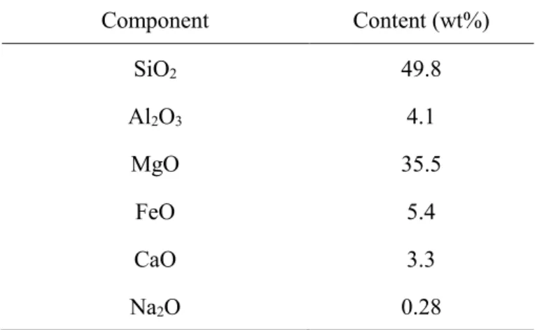
Our models assume that Venus’s crust is a uniform spherical shell. Previous studies reported small differences in the estimated crustal thickness and density of Venus based on different data and methods (e.g., Grimm and Solomon, 1988; Yang et al., 2016). Therefore, we set the parameters of the crust to fixed values considering the proportion of the crustal mass to the total mass of Venus. The thickness and density of the crust are set to 25 km and 2900 kg/m3_, respectively (Yang et al., 2016), the Lamé coefficients λ and μ are set to 56.4 and 35.8 GPa, respectively (Yoder, 1995), and the viscosity of the crust is fixed at 1021 _{Pa·s (Romeo and} Turcotte, 2008). For the mantle region, we consider that all parameters (density, seismic velocity, temperature, and viscosity) vary with depth instead of setting them to constant values. The isentropic temperature, radial density, P-wave velocity, and S-wave velocity are computed from the model of Venus’s mantle composition using the Perple_X program (Connolly, 2005) with the thermodynamic database stx11ver.dat (Stixrude and Lithgow-Bertelloni, 2011). The detailed calculation process can be found in Appendix A. The mantle composition in our models is estimated from the Morgan and Anders (1980) model (hereafter the M&A model) based on common fractionation processes in the solar nebula between terrestrial planets and chondrites, as listed in Table 1.

In our models, we assume varying temperatures at the CMB and varying thicknesses of the TBLb/TL; the temperatures in the TBLb and TL will change according to these two

Accepted

Article

parameters. For the “Cold” model case, we employ an isentropic temperature to approximate the mantle temperature profile; however, for the temperature in the TBLb, we use an error function as a less complicated approximation, as in the studies on the D’’ layer of Earth (e.g., Lay et al., 2006; van de Hilst et al., 2007). The mantle temperature profile for the “Cold” model case is calculated as follows:





( )

( )

(

)

1 erf (

)

r R

T r

T r

T

T R

h













_



_





where Ta(r)|T=1610K is the isentropic temperature extrapolated from the potential temperature

(Katsura et al. 2010), TCMB is the temperature at the CMB, RCMB is the core radius, and hTBLb is the thickness of the TBLb.

For the “Hot” model case, we assume that the temperatures of the harzburgite and basalt layers are both the isentropic temperature for simplicity. The difference is that the isentropic temperature of the basalt layer is extrapolated from the temperature of the CMB, whereas the isentropic temperature of the harzburgite layer is extrapolated from the potential temperature, similar to the “Cold” model case. We also use the error function to approximate the temperature in the TL. The mantle temperature profile for the “Hot” model case is calculated as follows:





CMB

Btop

Btop Btop Btop

1610K 1610K TL

( )

(

)

(

)

1 erf (

) ,

( )

( )

,

r

R

T r

T R

T R

r

R

h

T r

T r

r

R

































_



where Ta(r)|T=T_CMB is the isentropic temperature extrapolated from the TCMB, RBtop is the radius to the top of the basalt layer, and hTL is the thickness of the TL. Compared to the final state (i.e. 4.5 Gyr) of the mantle model given by O’Rourke et al. (2018), this simplification excluding the thin bottom thermal boundary layer will slightly increase the temperature in the basalt layer (see Figure S1) resulting in about 0.7% higher in synthetic tidal Love number k2.

A rapid increase in mantle temperature has an influence on the viscosity of the mantle. Instead of assuming the mantle viscosity to be constant, the mantle viscosity profile of our model is calculated from the temperature profile by using the following:

0

( )

( )=

exp

( )

g T r

r

T r







_







_





Accepted

Article

where Tm(r) is the melting temperature of bridgmanite (MgSiO3) and g’ is a dimensionless constant. Tm(r) is calculated using the results given by Di Paola and Brodholt (2016) and the

method proposed by Stixrude and Karki (2005), and we assume g’=12 (Steinberger and Calderwood, 2006). v0 is set to 1014 Pa·s, which results in a mantle viscosity profile similar to that of Earth (see Figure S3 (c)) on the order of 1019 _{to 10}21 _{Pa·s for the upper mantle and 10}21 to 1023 _{for the lower mantle (Čížková et al., 2012). By comparing with other} viscosity-temperature laws (e.g. the Arrhenius laws), we find that our profile is only slightly different from their results in the upper mantle (see Figure S2) resulting in tiny differences in the synthetic geodetic parameters (see Table S1), if the viscosity discontinuous between upper and lower mantles of Venus does not exist. Therefore, we regard that this method can provide a sufficient approximation of the variation in mantle viscosity with temperature.

2.2 Core

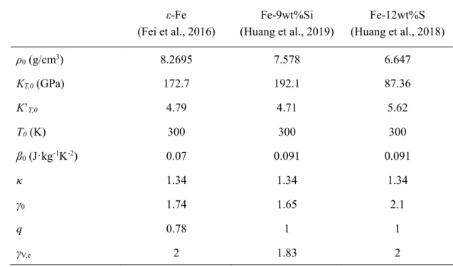
We use a third-order finite-strain Birch-Murnaghan equation of state (Birch, 1978) to compute the parameters for the core (see Appendix B). Rocky planets are generally believed to have Fe-rich metallic cores containing minor contents of light elements, which may be S, O, Si, C, or H. However, there is still controversy over which light element(s) are dissolved in the Earth’s core (e.g., Hirose et al., 2013). Hirose et al. (2013) suggested that the liquid core contains approximately 6 wt% Si, 3 wt% O, and 1-2 wt% S. Huang et al. (2019) provided evidence that the liquid core contains 5.6±3.0 wt% S and 3.8±2.9 wt% Si satisfying both geophysical and geochemical constraints. We assume that the light elements within the liquid core in our models are Si and S. We use three equation of state parameters, namely, ε-Fe (Fei et al., 2016), Fe-9Si (Huang et al., 2018), and Fe-12S (Huang et al., 2019), which were obtained from high-pressure experiments; the experiments are summarized in Table 2.

If we assume that these alloys are mixed ideally, the molar volume, isothermal bulk modulus, and thermal expansion of the mixture can be calculated as follows:

mix i i i

V







V

V

V







 

Accepted

Article

V

V

K







K

where χi is the molar fraction of each component (Fe, Fe-9Si, and Fe-12S) and Vi is the molar

volume. The αi value of each component is calculated by Eq. B6. We consider a 1% reduction

in density from the solid phase to the liquid phase (Huang et al., 2019). In our models, it is necessary to know the solidus temperature of the core to determine the presence of a solid inner core. Furthermore, the contents of light elements concentrated within the core affect the solidification temperature. Therefore, we use an approximation to simulate this effect, given by Anderson (1998) as follows:

Fe,melt ln(1 i) i

T T w

  



where wi is the molar fraction of each light element (S and Si). TFe,melt is the melting temperature of pure Fe obtained from Anzellini et al. (2013). We compare the results calculated using Eq. 7 and the experimental data of the Fe-S-Si ternary system given by Tateno et al. (2018). For the No. 8 run (P=128 GPa, 0.7 wt% Si and 5.6 wt% S) and No. 9 run (P=129 GPa, 1.6 wt% Si and 3.9 wt% S) of Tateno et al. (2018), the experimental melting temperatures are 3410±170 and 3570±180 K, respectively, whereas our estimated melting temperatures using Eq. 7 are 3640 and 3690 K, respectively. Hence, this approximation is suitable for the Fe-S-Si system, although the melting temperatures calculated by Eq. 7 are slightly overestimated with respect to the experimental data. The temperature of the core is approximated using the adiabatic temperature based on the specific heat CV and the effective Grüneisen parameter γeff of the Fe-S-Si mixture; these parameters rely on the additive law (Jing, 1986):

,mix ,vib ,e V i Vi i Vi i i C 









V

V

_









where CVi,vib and CVi,e are the vibrational and electronic specific heats, respectively, of each

component (Fe, Fe-9Si, and Fe-12S) and γeff,i is the effective Grüneisen parameter of each

component. If the temperature of the core is lower than the solidus temperature curve, the state of the core may convert from liquid to solid; by definition, this point represents the inner core boundary (hereafter ICB) of the model. Based on the study of Davies (2015), Si is partitioned

Accepted

Article

between solid and liquid Fe almost equally. Therefore, we assume that the inner core contains only Si and has the same amount of Si as the liquid core, in agreement with Huang et al. (2019). Considering the large range of viscosities of the Earth’s inner core proposed by previous studies (e.g., Reaman et al., 2011; Koot and Dumberry, 2011; Ritterbex and Tsuchiya, 2020), we study the possible influence of the solid inner core viscosity on k2. We find that the variation in the viscosity of an inner core surrounded by a liquid outer core has little impact on the synthetic value of k2, in agreement with the conclusion of Dumoulin et al. (2017). Thus, we simply assume that the viscosity of Venus’s inner core is 1021 _{Pa·s. In addition, the viscosity of} the liquid core is considered to be approximately 1.5×10-2 _{Pa·s (e.g., de Wijs et al., 1998);} however, the viscosity of the liquid core does not affect the calculation of the models’ tide parameters based on our calculation method (see Text S1).

2.3 Establishing the model

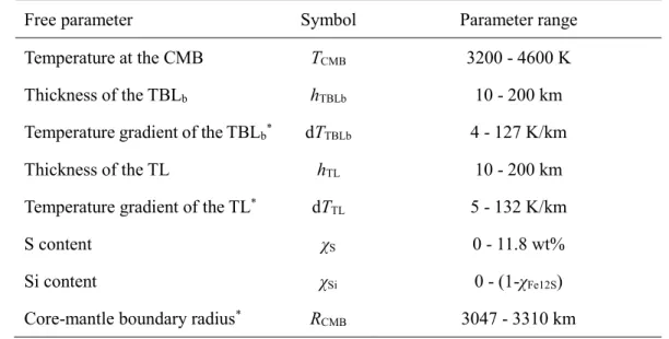
The free parameters in our model are the temperature at the CMB (TCMB), the thickness of the TBLb (hTBLb) (for the “Hot” model case, this is the thickness of the TL, hTL) and the S and Si contents of the liquid core. By adjusting these four free parameters, we obtain a series of models. The reference viscosity v0 is another parameter that controls the viscosity of the whole mantle; however, in the model generation phase, we consider only a fixed v0. The temperature at the CMB was considered by previous studies to be approximately 3600 K (Steinberger et al., 2010; Aitta, 2012). We therefore investigate a wide range of TCMB from 3200 to 4600 K. For the “Cold” model case, the thickness of the TBLb is assumed to range from 10 to 200 km, which is slightly thinner than the D” layer of the Earth (Lay et al., 2006; van de Hilst et al., 2007; Lay et al., 2008). Combining hTBLb and the difference between Ta(r) and TCMB, we obtain the temperature gradient within the TBLb (dTTBLb). Moreover, for the “Hot” model case, we assume that the thickness of the basalt layer is 1000 km (O’Rourke et al., 2018) for simplicity. Based on Eq. 2, we can use both the difference between the adiabatic temperature extrapolated from TCMB and the adiabatic temperature extrapolated from the potential temperature at the upper boundary of the basalt layer and the thickness of the TL to calculate the temperature gradient (dTTL). Similar to the thickness of the TBLb, the thickness of the TL is also assumed to range

Accepted

Article

from 10 to 200 km.

For the core, we assume that the S content of the liquid core ranges from 0 to 11.8 wt%, which is the upper limit of the S content in Fe-12S (Huang et al., 2019). The molar fraction of Fe-9Si is random, ranging from 0 to 1-χFe12S. In addition, the rest of the liquid core is composed of ε-Fe. The mass fraction of Si is calculated from χFe9Si, and the temperature profile of the core is calculated from TCMB.

We assume that the existence of a solid core depends on the calculated temperature profile and pressure-dependent melting temperature (TFe,melt+ΔT), as mentioned in Section 2.2. By adjusting the radius of the core, we ensure that the total mass and radius of each model are consistent with the observed radius and mass of Venus. The ranges of all free parameters are summarized in Table 3.

To calculate the tidal Love number k2, we perform numerical integration with the function y method (Saito, 1974), detailed in Text S1. To calculate k2, we employ the Andrade rheological model (Andrade, 1962), whose complex shear modulus is:

1 J



 

 







where μ is the unrelaxed shear modulus, ω is the tidal frequency, and ν is the viscosity. The parameter α represents the frequency dependence of the compliance, and β is the amplitude of the transient response. We utilize an approach similar to that of Dumoulin et al. (2017), who assumed that α=0.2-0.3 and β=μα-1_ν-α_{. The differences in calculating k}

2 and Q, which are caused

by varying α (0.25±0.05), are regarded as uncertainties.

2.4 Observed geodetic data

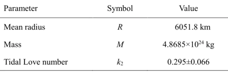
In this study, we employ Venus’s mean radius R (Seidelmann et al., 2007), Venus’s total mass M (Lodders and Fegley, 1998), and the degree-two tidal Love number k2 with a primary tidal flexing period of 58.4 days (Konopliv and Yoder, 1996). These values are summarized in Table 4. The current observed tidal Love number k2=0.295 ± 0.066 (Konopliv and Yoder, 1996) was estimated from Doppler tracking data of the Pioneer Venus Orbiter (PVO, from December

Accepted

Article

1978 to September 1982) and Magellan spacecraft (from September 1992 to October 1994). However, the MoI was not well determined due to the lack of observation data from Venus and the extremely slow rotation of the planet (Kaula, 1979). In previous studies, the normalized MoI was widely considered to be approximately 0.33 (Yoder, 1995; Mocquet et al., 2011), while the MoI values estimated from different models ranged from 0.327 to 0.341 (Yoder, 1995; Zhang and Zhang, 1995; Lodders and Fegley, 1998; Aitta, 2012; Dumoulin et al., 2017). The uncertainty in Venus’s GM obtained from the MGNP180U model is extremely small (Konopliv et al., 1999). Thus, in our models, the total mass and radius are fixed to the observed mass of M=4.8685×1024 _{kg and a mean radius of R=6051.8 km. Consequently, the average density of} each model is the same. In addition, the tidal dissipation factor Q relates to the phase lag ε and is expressed as Q-1_{=sin(ε). The phase lag of the Earth’s tide can be obtained by combining} satellite orbital tracking and altimetry data (Ray et al., 1996). Unfortunately, the tidal dissipation factor Q of Venus’s tide is still unknown. As a reference, the Q of Earth extrapolated to Venus’s tidal period (58.4 days) is considered to be approximately 100 (Tobie et al., 2019).

2.5 Validation of the method

We apply our method to a model of Earth to validate the “Cold” model case. The mean crustal density is assumed to be 2830 kg/m3 _{with a crustal thickness of 40 km (not considering} oceanic crust). The composition of Earth’s mantle is assumed to be essentially pyrolite (McDonough and Sun, 1995). We use the Perple_X program to compute the mantle parameters. The composition of the Earth’s core is assumed to be the same as that presented in Section 2.2: the liquid outer core contains both S and Si, and the inner core contains the same Si content as the liquid outer core. The temperature at the CMB is considered to range from 3850 to 4600 K (Fischer, 2016), and the thickness of the D’’ layer ranges from 150 to 300 km (van de Hilst et al., 2007). The ICB radius is determined by the temperature, and the CMB radius is adjusted to comply with the total mass of Earth (5.972×1024 _kg).

With a Si content of 3.8 wt%, a S content of 5.3 wt%, and a CMB temperature of 3910 K, the model matches PREM well (see Figure S3); the CMB radius and ICB radius are 3480 km and 1209 km, respectively. We further use this model to study the influence of varying α. The

Accepted

Article

k2 of the Earth’s M2 (semidiurnal) period is considered to be 0.30102-0.0013i (McCarthy and Petit, 2004), while Q is approximately 280 (Ray et al., 2001), and the MoI is 0.3307 (Williams, 1994). In M2 tidal period, the synthetic k2 values (0.3020-0.3043) with α varying from 0.24 to

0.3 match the observed values (<1% error); similarly, the synthetic Q values (232-354) withα varying from 0.24 to 0.28 are within the error of Q (230-360) and are in agreement with the Q values of the Mf (fortnightly) period (Ray and Egbert, 2012) and Chandler wobble period (Furuya and Chao, 1996). The synthetic MoI is 0.33, which agrees with the observations. Therefore, our proposed method can provide a sufficient approximation model for Venus.

3. Results and Analysis

To calculate the synthetic geodetic parameters of Venus, including the tidal Love number k2, mean MoI, and tidal dissipation factor Q, our model was discretized into 1 km uniform spherical shells. The depth-dependent parameters (density, seismic velocities, viscosity, and temperature) of each layer were computed by the methods described in Section 2. We generated 400 different models matching the total mass of Venus, including 100 models with an SIC. All acceptable models are available in the data repository of Xiao (2019). The radial parameters of the models are shown in Figure 2.

As seen from Figures 2(a) and 2(e), the core radii of the models with an SIC are slightly lower than those of the models without an SIC, due to the different core densities. Figures 2(c) and 2(f) similarly indicate that the core temperatures of the models with an SIC are generally lower than those of the models without an SIC. When TCMB exceeds ~4000 K, the model core is completely liquid; when TCMB is between 3600 and 4000 K, the core is partly solidified; when TCMB is less than ~3600 K, the model contains an SIC. From Figure 2(a), we deduced that the CMB radii for the “Cold” models with an SIC range from 3047 to 3229 km, as the solid inner core ranges from 589 to 2971 km; in contrast, the CMB radii for the “Cold” models without an SIC range from 3102 to 3306 km. The lower limit of the thickness of the liquid outer core is 136 km due to our model assumptions. As shown in Figure 2(d), according to our assumed v0=1014 Pa·s, the lower limit of the viscosity in the TBLb is approximately 1019 Pa·s for the models without an SIC and approximately 1020 _{Pa·s for the models with an SIC.}

Accepted

Article

For the “Hot” model case, the CMB radii of the models with an SIC range from 3090 to 3284 km with an inner core radius of 548 to 3073 km, whereas the core radii of the models without an SIC range from 3128 to 3331 km, as shown in Figure 2(e). The CMB radii for the “Hot” model case are slightly larger than those for the “Cold” model case due to the mantle density deficit caused by the high temperature. The mantle temperatures of some models are higher than the melting temperature of the bridgmanite (Tm), due to the extremely high temperature at the CMB.Weartificially excluded these models during model generation as the mantle of all models in the “Cold” model case are completely solid. With the upper limit of TCMB of 4336 K (“Hot” model case), the mantle temperatures of all models are lower than the melting temperature, as shown in Figure 2(g). From Figure 2(h), based on our assumed v0=1014 Pa·s, the viscosity of the basalt layer for the models with an SIC is similar to the viscosity profile given by Armann and Tackley (2012); however, the viscosity of the basalt layer for the models without an SIC is reduced due to the high temperature.

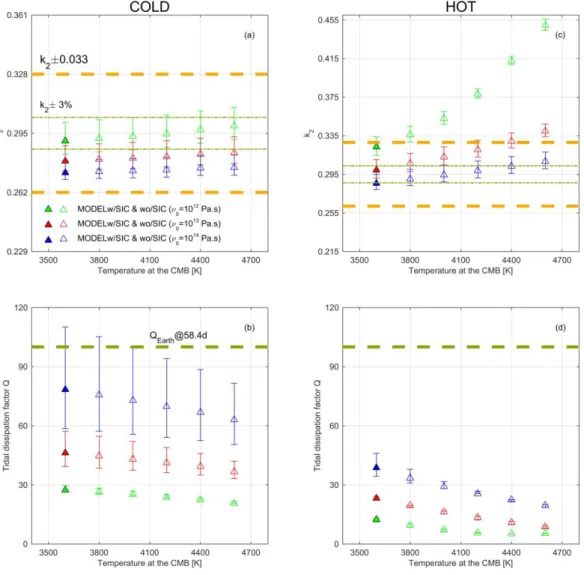
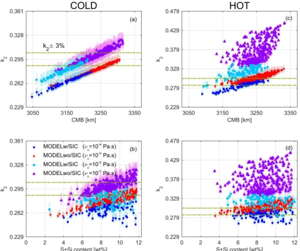
We calculated the synthetic tidal Love number k2 and MoI, using the radial parameters (density, seismic velocity, and viscosity) for each model. The tidal dissipation factor Q is the ratio of the modulus of k2 to the imaginary part of k2. The synthetic geodetic data (k2, MoI, and Q) of the models are shown in Figures 3-5. In addition to k2 obtained from PVO and Magellan missions, we also plotted the uncertainty in the highly precise k2 expected to be obtained by EnVision mission for comparison.

As shown in Figure 3, the synthetic k2 values of all the models (v0=1014 Pa·s) based on the M&A mantle composition model are located within the uncertainties (±0.066) in the observed data. Moreover, the uncertainties in the current observations are greater than the boundaries of our self-consistent model. In addition, the range of synthetic k2 for the “Hot” model case is

generally larger than that for the “Cold” model case. As shown in Figures 3(a) and 3(e), increasing the CMB radius has a significant influence on the synthetic k2 for both cases, and

Figures 3(b) and 3(f) demonstrate that the synthetic k2 is also affected by the CMB temperature.

Nevertheless, for the “Cold” model case, the CMB temperature has a relatively minor influence on k2 relative to the CMB radius, whereas for the “Hot” model, TCMB has an influence on the synthetic k2 comparable to that of the CMB radius. This is because the viscosity of the basalt

Accepted

Article

Some models exhibit a high TCMB with a low synthetic k2. The cores of these models, which

contain smaller light element contents (S+Si < 4 wt%), are still completely liquid due to the very high temperature of the core. Such a dense liquid core results in a decrease in the core radius, which reduces the synthetic k2. Consequently, the CMB temperature is a decisive factor for the existence of the solid inner core for the “Cold” model case. The dots corresponding to the models with and without an SIC are separated from each other in Figure 3(b). However, for the “Hot” model case, there is some overlap between the dots of the models with and without an SIC, as shown in Figure 3(f).

In Figures 3(c) and 3(g), we show only the effect of the total light element content on the synthetic k2 due to the similar effects of the S and Si contents on the density deficit of the Fe alloy. The variation in the light element content within the core also significantly influences the synthetic k2. The light element content in the core strongly affects the size of the core to satisfy the total mass of Venus. In addition, the models with and without an SIC have different contents of light elements: the light element content ranges from 4.0 to 11.7 wt% in the model with an SIC and from 2.6 to 11.8 wt% in the model without an SIC. In contrast, the thickness of the TBLb or TL has almost no influence on the synthetic k2, as shown in Figures 3(d) and 3(h).

As shown in Figure 4, the synthetic tidal dissipation factor Q (v0=1014 Pa·s) values vary between the “Cold” and “Hot” model cases based on the M&A mantle composition model. The synthetic Q values for the “Cold” model case range from 63 to 83, whereas the Q for the “Hot” model case ranges from 21 to 54. For a certain α, the hTBLb for the “Cold” model case has a significant influence on the synthetic Q, while the synthetic Q for the “Hot” model case is more affected by TCMB, as seen in Figures 4(d) and 4(f). For the “Cold” model case, the effect of varying hTBLb on Q is smaller than the effect of the uncertainty caused by α; however, for the “Hot” model case, even considering the uncertainty caused by α, the effect of varying TCMB on Q is still obvious.

For both the “Cold” and the “Hot” model cases, the synthetic Q values of the models without an SIC are generally less than those of the models with an SIC. In addition, for the “Hot” model case, the synthetic Q values of the models with and without an SIC differ from each other, as shown in Figure 4(g). However, considering the large uncertainties caused by different α, this difference is still inadequate to constrain the state of the core.Theother figures

Accepted

Article

show that the synthetic Q does not change significantly with the CMB radius and light element content.

The synthetic MoI values for both the “Cold” and the “Hot” model cases range from 0.331 to 0.335, which are slightly larger than the previous value (~0.33) estimated from an Earth-like Venus model (Yoder, 1995). However, the synthetic MoI values do not exceed the range of MoI values (between 0.327 and 0.341) obtained from the different models discussed in previous studies. Moreover, there is almost no difference between the MoI values for the “Cold” and “Hot” model cases. However, slight differences are observed for the models with an SIC, in which the MoI values for the “Hot” model case are slightly larger than those for the “Cold” model case. As shown in Figures 5(a), 5(c), 5(e) and 5(g), variations in the core radius and the light element content of the liquid core influence the synthetic mean MoI, and the CMB temperature has a minor influence on the synthetic MoI, as shown in Figures 5(b) and 5(f). In contrast, Figures 5(d) and 5(h) indicate that neither the TBLb thickness nor the TL thickness has an influence on the synthetic MoI. There is an overlap between the synthetic MoI values of the models with and without an SIC, demonstrating that it is impossible to distinguish these two types of models solely by using the MoI.

Based on this analysis of the effects of four free parameters (core radius, temperature at the CMB, light element content, and thickness of the TBLb/TL) on the values of k2, Q and MoI, we found that it is nearly impossible to constrain the internal structure of Venus using the currently observed k2 because of its considerable uncertainty. Furthermore, determining the existence of an SIC using currently observed data of Venus is also difficult. However, we discovered that the synthetic k2 and Q values calculated by our models obviously differ in

response to variations in TCMB. Therefore, we further analyzed the effect of varying TCMB on the synthetic k2 and Q.

We fixed the radius of the core at 3200 km and the TBLb/TL thickness at 150 km and calculated the synthetic k2 and Q values at six different values of TCMB (3600, 3800, 4000, 4200, 4400, and 4600 K). Additionally, we analyzed the effects of different v0 values on the synthetic k2 and Q by considering that the range of the synthetic k2 with a given v0=1014 Pa·sis less than the observed uncertainty in k2. We therefore considered three different cases of v0 (v0=1012, 1013, and 1014 _{Pa·s). The results are shown in Figure 6.}

Accepted

Article

As shown in Figure 6, when the core radius is fixed, the synthetic k2 will increase and the synthetic Q will decrease, as TCMB increases. However, it is difficult to constrain the temperature at the CMB by using a set of k2 and Q because there is a small trade-off between TCMB and the mantle viscosity structure, which depends strongly on v0. A given set of k2 and Q may correspond to a model with high TCMB but a harder mantle (high v0) or a model with low TCMB but a softer mantle (low v0).

The effects of TCMB on the synthetic k2 and Q corresponding to different viscoelastic structures differ significantly. Figure 6(a) shows that an increase in TCMB results in an increase in k2, and the magnitude of this variation is amplified as v0 decreases based on the assumption that Venus’s mantle is similar to Earth’s mantle. In the case of v0=1012 Pa·s, this effect is obvious. The difference in the synthetic k2 due to an increase in TCMB from 3600 to 4600 K is approximately 0.01, which is comparable to the uncertainty caused by α. However, an increase in TCMB also results in a decrease in Q, and the magnitude of this variation is reduced as v0 decreases, as shown in Figure 6(b). For the “Hot” model case, the responses of k2 and Q to TCMB and v0 are almost the same as those for the “Cold” model case. Thus, we can rule out some combinations of TCMB and v0 for a given set of k2 and Q for both the “Cold” and the “Hot” model cases. For example, under the condition of Q=30±10 and k2=0.295±0.1, most of the “Cold” models with v0>1013 Pa·s are excluded; among the “Hot” models, only those with v0 ~ 1014 Pa·s and TCMB<4400 K are included.

Furthermore, the synthetic Q values for the “Hot” model case are much lower than those for the “Cold” model case. If the observed Q value is large (i.e., Q=100) with k2=0.295, the "Hot" model case will be excluded. Hence, the combination of Q and k2 can provide evidence for Venus’s mantle structure obtained by other methods (such as simulations of thermal evolution).

We also performed a simulation of our models considering a more precise k2. The EnVision mission under consideration by the European Space Agency (ESA) could improve the measurements of tidal parameters relative to those made during the Magellan mission (Ghail et al., 2016) and will reduce the uncertainty in k2 to 3% (Rosenblatt, 2019). We also considered different v0 values, but for clarity, we show only the results for v0=1012 and 1014 Pa·s in Figure 7.

Accepted

Article

As shown in Figure 7, with the uncertainty in k2 reduced from ±0.033 to ±0.00885 (3% of 0.295), the acceptable model space is also greatly reduced. Based on the assumption that k2 equals 0.295 and with the M&A mantle composition model, for the “Cold” model case, most of the models with an SIC and a hard mantle (v0=1014 Pa·s) are excluded even if we consider the uncertainties caused by varying α. In addition, models with a low light element content are also excluded; for instance, the light element contents of the models with v0=1012 Pa·s should exceed 3 wt%, and the light element contents of the models with v0=1014 Pa·s should exceed 6.5 wt%. For the “Hot” model case, most of the models with a soft mantle (v0=1012 Pa·s) but without an SIC are excluded. Furthermore, when v0=1014 Pa·s, the estimated range of the core radius is reduced to 3120-3290 km for the “Hot” model case (3220-3310 km for the “Cold” model case). Of course, the exclusion of models and the estimation of parameters depend on the exact obtained value of k2. If k2 isless than 0.26, “Cold” models with a hard mantle are included, whereas models with a soft mantle are excluded. Nevertheless, despite the improved precision of k2, it will still be difficult to rule out the existence of an SIC because v0 cannot be uniquely determined by external measurements.

4. Discussion

In this study, we investigated several models of Venus by considering various temperatures at the CMB, various thicknesses of the TBLb/TL, and various light element contents of the liquid core. Although present-day observed geodetic data cannot constrain the temperature at the CMB, we found that the region at the bottom of Venus’s mantle may not be the same as that at the bottom of Earth’s mantle, based on the M&A mantle composition model.

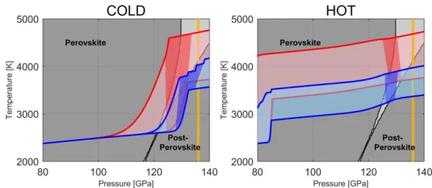
In recent studies of the D’’ layer of Earth, the discontinuities in seismic wave velocities were related to the phase transition of perovskite (Lay et al., 2006; van der Hilst et al., 2007; Kawai and Tsuchiya, 2009). Accordingly, we generated a phase diagram including perovskite (Pv) and post-perovskite (pPv) and compared the diagram with the pressure-dependent temperature profiles of our models; the results are shown in Figure 8.

As shown in Figure 8, all the pressure-dependent temperature profiles above the CMB in our models are in the region of perovskite stability. Thus, in our models, no phase transition

Accepted

Article

occurs in the lowermost mantle of Venus. Our results may indicate that the composition of Venus’s lowermost mantle may be different from the composition of the D’’ layer of Earth based on the M&A mantle composition model. The difference, however, depends heavily on the chosen mantle composition model. Therefore, we further considered three other mantle composition models (Dumoulin et al., 2017), which are summarized in Table S2, and analyzed the influence of different composition models on the TBLb. These three models represent Fe-depleted (V1, 0.24 wt% FeO), Earth-like (V2, 8.1 wt% FeO), and Fe-rich (V3, 18.7 wt% FeO) mantle, respectively. The results are shown in Figures S4-S6.

Composition models V1 and V2 have no impacts on our conclusions; the pressure-dependent temperature profiles above the CMB in all models are in the region of perovskite stability, as shown in Figures S4 and S5. However, for model V3, which results in a much smaller core and a denser mantle, the pressure-dependent temperature profiles for the “Cold” model case cross the border between the perovskite phase and the post-perovskite phase, as shown in Figure 9. This finding indicates that if Venus has an Fe-rich mantle, a phase transition from perovskite to post-perovskite is still possible at the bottom of the mantle. In addition, we calculated the synthetic Fe abundance for the models, and the results are summarized in Table 5.

However, some problems arise with model V3 when considering the abundance of Fe in Venus (Morgan and Anders, 1980). Based on our assumption about the light elements contained within Venus’s core, the Fe abundance in the models considering V3 for the mantle composition is approximately 16% larger than the Fe abundance of 31.17 wt% given by Morgan and Anders (1980). To reduce the Fe content, the core needs to contain more light elements, which will increase the core radius and decrease the pressure at the CMB. Considering the scarcity of high-temperature and high-pressure experimental data, we cannot quantitatively model an increase in the core radius caused by a higher content of light elements inside the core.

5. Conclusion

We built two types of Venus interior models: An Earth-like “Cold” model case and a “Hot” model case with higher mantle temperature. We considered various temperatures at the CMB,

Accepted

Article

various light element contents (S+Si) within the liquid core, and various thicknesses of the TBLb/TL based on the mantle composition model from Morgan and Anders (1980). The radial density and seismic velocity of the mantle were computed from the mantle composition model by using the Perple_X program. The radial viscosity was given by mantle temperature profiles. The radial parameters of the core (both liquid and solid cores) were computed following the third-order Birch-Murnaghan equation of state and the thermal pressure model. We calculated the synthetic k2 values of these models and compared the results against current observed data. Based on our model assumptions, the synthetic k2 values of all the models were in agreement with the currently observed k2 data. Therefore, the internal structure of Venus cannot be effectively constrained by observed geodetic data at present due to the large uncertainty in k2. It is also difficult to constrain the state of the core because the upper limit of the synthetic k2 excluding the existence of a solid inner core strongly depends on the reference mantle viscosity v0. However, based on our model assumptions, it is still possible to rule out some combinations of the thermal structure and viscous structure by combining k2 and Q if the core radius is reliably determined. Furthermore, we provided evidence that the combination of observed k2 and Q can distinguish whether the mantle of Venus is similar to Earth’s so long as the observational value of Q can be obtained.

In this study, we also investigated the differences between the lowermost mantle of Venus and the D” layer of Earth. For the “Cold” model case, we assumed a high temperature gradient layer at the bottom of Venus’s mantle. The temperature and pressure conditions in the TBLb are not sufficient to accommodate a phase transition from perovskite to post-perovskite based on the M&A mantle composition model. The absence of post-perovskite may potentially indicate that the composition of Venus’s TBLb may be different from the composition of Earth’s D” layer. This inference is valid for the Venus models with an Earth-like or Fe-depleted mantle composition (FeO < 8.1 wt%). In contrast, if Venus has an Fe-rich mantle, a phase transition from perovskite to post-perovskite is still possible at the bottom of the mantle. Seismic data from future exploration missions on Venus (for example, the mission discussed at the Keck Institute for Space Studies; Stevenson et al., 2015) are required to obtain a more refined constraint on Venus’s deep mantle structure. In particular, these constraints will help to confirm whether the deep mantle composition of Venus is different from that of Earth’s D” layer.

Accepted

Article

Among the projected exploration missions of Venus, the EnVision mission and VERITAS mission (Smrekar et al., 2019) might improve the tidal measurements compared to those made during the Magellan mission. If the mission precision goals are fulfilled, this improvement can further reduce the size of the model space. This improvement will also contribute to estimating the mantle viscosity structure. In addition, if the tidal dissipation factor Q can be obtained, we will be more capable of confirming whether a thermal boundary layer exists at the bottom of Venus’s mantle. The seismic data expected from future missions will provide information on the deep mantle of Venus, which will contribute to a better understanding of the thermal evolution of Venus and help to understand why the evolutionary characteristics of Venus and Earth are so different.

Acknowledgment: We sincerely appreciate the four reviewers (including Prof. William B. Moore) and the editor (Prof. Laurent G. J. Montesi) for their constructive comments, which greatly improved our submission manuscript. We also acknowledge Prof. Haijun Huang for his valuable discussion and suggestions. The Perple_X program for computing radial isentropic temperature, density, and seismic velocities is available at http://www.perplex.ethz.ch. This work is supported by the National Scientific Foundation of China (U1831132, 41874010), the Innovation Group of Natural Fund of Hubei Province (2018CFA087), and Open Funding of Macau University of Science and Technology (FDCT 119/2017/A3). M. Gregoire is supported by funding from the National Centre of Scientific Research (CNRS); Y. Harada is supported by the Research Funding Projects (No. 007/2016/A1, No. 119/2017/A3, and No. 187/2017/A3) at the Science and Technology Development Fund, the Macau Special Administrative Region; and J.P. Barriot is supported by a DAR grant in planetology from the French Space Agency (CNES); All data associated with this manuscript are available in the Harvard Dataverse of Xiao (2019).

Accepted

Article

Appendix A: Temperature-dependent density

Unlike Earth, Venus does not have a widely accepted reference model. We used the Perple_X program (Connolly, 2005) to calculate the density and seismic velocity of Venus’s mantle based on the M&A composition model (Table 1 in the main text). To obtain the isentropic temperature, we first used Perple_X to calculate the entropy of our mantle composition over a temperature range from 1400 to 2700 K and a pressure range from 0.2 to 140 GPa. Then, we obtained the isentropic P-T path along s=2540 J·K-1_·kg-1 _{to ensure that the} mantle isentropic temperature extrapolated to the surface was consistent with the mantle potential temperature of 1610 K (Katsura et al. 2010).

For each model, the CMB radius must be adjusted to fit the total mass and mean radius of Venus, and the P-T relationship of the TBLb is varied during the iterations. It is difficult to calculate the parameters along the P-T path for every step of the iteration. However, the density reduction within the TBLb due to the temperature increase (relative to the isentropic temperature) should be taken into consideration. Thus, we used a simplified approximation. First, we did not consider the phase transition by excluding pPv from the endmember in the build file of Venus’s mantle. Then, we obtained the density, seismic velocity, and thermal expansion coefficient α along the isentropic temperature. The effect of the density reduction caused by temperature is approximated as follows:

exp(

(

))

a

T

T

 









We obtained the P-T relations of the models by applying Eq. A1 to the iteration. Then, we included pPv in the build file and recalculated the density along this final P-T relation. This approximation was in good agreement with the results obtained by Perple_X. No phase transition from Pv to pPv occurred along any P-T path.

Accepted

Article

Appendix B: Third-order Birch-Murnaghan equation of state

We employed the third-order finite-strain Birch-Murnaghan equations of state to calculate the parameters of the core. The third-order finite-strain Birch-Murnaghan equations of state are written as: 5 2 300 ,0 ,0 ,0

3

3 (1 2 )

(

4)

2

P



f



f



_

K



K

K





f



_





27

( ,

)

(1 2 )

(3

5)

(

4)

2

K P T

 

f

_



K



K

K





f



K

K





f



_





( ,

P T

)

(1 2 )

f









where f is the negative Euler strain, KT(P,T0) is the isothermal bulk modulus at the reference temperature T0, and KT,0 and K’T,0 are the isothermal bulk modulus and its pressure derivative, respectively, under standard conditions. Using Eqs. B1 and B3, we obtained the isothermal P-ρ relation at 300 K. Then, we used the thermal pressure model given by Fei et al. (2016) to calculate the thermal pressure at the target temperature. The thermal pressure is calculated as follows: , 300 d 300 d T T vib e th V vib Ve P C T C T V V





_

_

where γvib=γ0 (ρ0/ρ)q and γe are the vibrational and electronic Grüneisen parameters, respectively. At high temperature, CV,vib≈3R/μ and CV,e=β0 (ρ0/ρ)kT are the vibrational and electronic specific heat, respectively, where R is the universal gas constant and μ is the molar mass. The parameters of each alloy are listed in Table 2. Then we obtained the relationship between ρ(P,T) and P(T) -P300K=Pth(T). We also obtained the relationship between the KT(P,T) and P(T). The adiabatic bulk modulus KS=KT(1+αγeffT), the effective Grüneisen parameter γeff and the thermal expansion coefficient α are calculated via the following equations:

,

(

)

C

C

C











C

VK







where CV= CV,vib+CVe. Using the above equations, we obtained ρ and KS at a specific P-T condition from the reference condition. The adiabatic temperature of the core can be obtained

Accepted

Article

by the following equation:

eff S

T

gT

r

K







_{ }



Accepted

Article

Reference

Aitta A. Venus’ internal structure, temperature and core composition. Icarus, 2012, 218(2): 967-974.

Andrade E N. The validity of the t1/3 _{law of flow of metals. Philosophical Magazine, 1962,}

7(84): 2003-2014.

Anderson O L. The Grüneisen parameter for iron at outer core conditions and the resulting conductive heat and power in the core. Physics of the Earth and Planetary Interiors, 1998, 109(3-4): 179-197.

Arkani-Hamed J, Toksöz M N. Thermal evolution of Venus. Physics of the Earth and Planetary Interiors, 1984, 34(4): 232-250.

Armann M, Tackley P J. Simulating the thermochemical magmatic and tectonic evolution of Venus’s mantle and lithosphere: Two-dimensional models. Journal of Geophysical Research: Planets, 2012, 117(E12).

Anzellini S, Dewaele A, Mezouar M, et al. Melting of iron at Earth’s inner core boundary based on fast X-ray diffraction. Science, 2013, 340(6131): 464-466.

Birch F. Finite strain isotherm and velocities for single-crystal and polycrystalline NaCl at high pressures and 300 K. Journal of Geophysical Research, 1978, 83(B3): 1257-1268. Canup R M, Asphaug E. Origin of the Moon in a giant impact near the end of the Earth’s

formation. Nature, 2001, 412(6848): 708.

Čížková H, van den Berg A P, Spakman W, et al. The viscosity of Earth’s lower mantle inferred from sinking speed of subducted lithosphere. Physics of the Earth and Planetary Interiors, 2012, 200: 56-62.

Connolly J A D. Computation of phase equilibria by linear programming: a tool for geodynamic modeling and its application to subduction zone decarbonation. Earth and Planetary Science Letters, 2005, 236(1-2): 524-541.

Davies J H. Did a mega-collision dry Venus' interior? Earth and Planetary Science Letters, 2008, 268(3-4): 376-383.

Davies C J. Cooling history of Earth’s core with high thermal conductivity. Physics of the Earth and Planetary Interiors, 2015, 247: 65-79.

de Wijs G A, Kresse G, Vočadlo L, et al. The viscosity of liquid iron at the physical conditions of the Earth's core. Nature, 1998, 392(6678): 805.

Di Paola C, Brodholt J P. Modeling the melting of multicomponent systems: the case of MgSiO3 perovskite under lower mantle conditions. Scientific Reports, 2016, 6: 29830.

Dumberry M, Rivoldini A. Mercury’s inner core size and core-crystallization regime. Icarus, 2015, 248: 254-268.

Dumoulin C, Tobie G, Verhoeven O, et al. Tidal constraints on the interior of Venus. Journal of Geophysical Research: Planets, 2017, 122(6): 1338-1352.

Dziewonski A M, Anderson D L. Preliminary reference Earth model. Physics of the Earth and Planetary Interiors, 1981, 25(4): 297-356.

Elsasser W M. Hydromagnetic dynamo theory. Reviews of Modern Physics, 1956, 28(2): 135. Fei Y, Murphy C, Shibazaki Y, et al. Thermal equation of state of hcp‐iron: Constraint on the density deficit of Earth's solid inner core. Geophysical Research Letters, 2016, 43(13): 6837-6843.

Accepted

Article

Fischer R A. Melting of Fe Alloys and the Thermal Structure of the Core. Deep Earth: Physics and Chemistry of the Lower Mantle and Core, 2016, 217: 1.

Florensky C P, Ronca L B, Basilevsky A T, et al. The surface of Venus as revealed by Soviet Venera 9 and 10. Geological Society of America Bulletin, 1977, 88(11): 1537-1545. Furuya M, Chao B F. Estimation of period and Q of the Chandler wobble. Geophysical Journal

International, 1996, 127(3): 693-702.

Genova A, Goossens S, Mazarico E, et al. Geodetic Evidence That Mercury Has A Solid Inner Core. Geophysical Research Letters, 2019, 46(7): 3625-3633.

Ghail R, Wilson C F, Widemann T. Envision M5 Venus orbiter proposal: Opportunities and challenges. AAS/Division for Planetary Sciences Meeting Abstracts# 48. 2016, 48. Grimm R E, Solomon S C. Viscous relaxation of impact crater relief on Venus: Constraints on

crustal thickness and thermal gradient. Journal of Geophysical Research: Solid Earth, 1988, 93(B10): 11911-11929.

Harada Y, Goossens S, Matsumoto K, et al. Strong tidal heating in an ultralow-viscosity zone at the core-mantle boundary of the Moon. Nature Geoscience, 2014, 7(8): 569.

Harada Y, Goossens S, Matsumoto K, et al. The deep lunar interior with a low-viscosity zone: Revised constraints from recent geodetic parameters on the tidal response of the Moon. Icarus, 2016, 276: 96-101.

Hirose K, Labrosse S, Hernlund J. Composition and state of the core. Annual Review of Earth and Planetary Sciences, 2013, 41: 657-691.

Huang H, Leng C, Wang Q, et al. Measurements of Sound Velocity of Liquid Fe‐11.8 wt% S up to 211.4 GPa and 6,150 K. Journal of Geophysical Research: Solid Earth, 2018, 123(6): 4730-4739.

Huang H, Leng C, Wang Q, et al. Equation of State for Shocked Fe‐8.6 wt% Si up to 240 GPa and 4,670 K. Journal of Geophysical Research: Solid Earth, 2019, 124(8): 8300-8312. Jing, F. Q. Introduction to Experimental Equation of State (in Chinese), 2nd ed., 371 pp.,

Scientific Press, Beijing, 1986.

Katsura T, Yoneda A, Yamazaki D, et al. Adiabatic temperature profile in the mantle. Physics of the Earth and Planetary Interiors, 2010, 183(1-2): 212-218.

Kaula W M. The moment of inertia of Mars. Geophysical Research Letters, 1979, 6(3): 194-196.

Kaula W M. Venus: A contrast in evolution to Earth. Science, 1990, 247(4947): 1191-1196. Kaula W M. The tectonics of Venus. Philosophical Transactions of the Royal Society of London.

Series A: Physical and Engineering Sciences, 1994, 349(1690): 345-355.

Kawai K, Tsuchiya T. Temperature profile in the lowermost mantle from seismological and mineral physics joint modeling. Proceedings of the National Academy of Sciences, 2009, 106(52): 22119-22123.

Khan A, Liebske C, Rozel A, et al. A geophysical perspective on the bulk composition of Mars. Journal of Geophysical Research: Planets, 2018, 123(2): 575-611.

Knapmeyer M. Planetary core size: A seismological approach. Planetary and Space Science, 2011, 59(10): 1062-1068.

Konopliv A S, Yoder, C F. Venusian k2 tidal Love number from Magellan and PVO tracking data. Geophysical Research Letters. 1996, 23, 1857–1860.

Accepted

Article

1999, 139(1): 3-18.

Koot L, Dumberry M. Viscosity of the Earth's inner core: Constraints from nutation observations. Earth and Planetary Science Letters, 2011, 308(3-4): 343-349.

Ksanfomaliti L V, Zubkova V M, Morozov N A, et al. Microseisms at the VENERA-13 and VENERA-14 Landing Sites. Soviet Astronomy Letters, 1982, 8: 241.

Lay T, Hernlund J, Garnero E J, et al. A post-perovskite lens and D” heat flux beneath the central Pacific. Science, 2006, 314(5803): 1272-1276.

Lay T, Hernlund J, Buffett B A. Core–mantle boundary heat flow. Nature geoscience, 2008, 1(1): 25.

Lodders K, Fegley B. The planetary scientist's companion. Oxford University Press on Demand, 1998.

Matsumoto K, Yamada R, Kikuchi F, et al. Internal structure of the Moon inferred from Apollo seismic data and selenodetic data from GRAIL and LLR. Geophysical Research Letters, 2015, 42(18): 7351-7358.

McCarthy D D, Petit G. IERS conventions (2003). IERS Technical Note, 2004.

McDonough W F, Sun S -s. The composition of the Earth. Chemical Geology, 1995, 120(3-4): 223-253.

Mocquet A, Rosenblatt P, Dehant V, et al. The deep interior of Venus, Mars, and the Earth: A brief review and the need for planetary surface-based measurements. Planetary and Space Science, 2011, 59(10): 1048-1061.

Morgan J W, Anders E. Chemical composition of earth, Venus, and Mercury. Proceedings of the National Academy of Sciences, 1980, 77(12): 6973-6977.

Nakada M, Iriguchi C, Karato S. The viscosity structure of the D” layer of the Earth’s mantle inferred from the analysis of Chandler wobble and tidal deformation. Physics of the Earth and Planetary Interiors, 2012, 208: 11-24.

Nakajima M, Stevenson D J. Melting and mixing states of the Earth's mantle after the Moon-forming impact. Earth and Planetary Science Letters, 2015, 427: 286-295.

Nimmo F. Why does Venus lack a magnetic field? Geology, 2002, 30(11): 987-990.

O’Rourke J G, Gillmann C, Tackley P. Prospects for an ancient dynamo and modern crustal remanent magnetism on Venus. Earth and Planetary Science Letters, 2018, 502: 46-56. Ray R D, Eanes R J, Chao B F. Detection of tidal dissipation in the solid Earth by satellite

tracking and altimetry. Nature, 1996, 381(6583): 595-597.

Ray R D, Eanes R J, Lemoine F G. Constraints on energy dissipation in the Earth's body tide from satellite tracking and altimetry. Geophysical Journal International, 2001, 144(2): 471-480.

Ray R D, Egbert G D. Fortnightly Earth rotation, ocean tides and mantle anelasticity. Geophysical Journal International, 2012, 189(1): 400-413.

Reaman D M, Daehn G S, Panero W R. Predictive mechanism for anisotropy development in the Earth's inner core. Earth and Planetary Science Letters, 2011, 312(3-4): 437-442. Ritterbex S, Tsuchiya T. Viscosity of hcp iron at Earth’s inner core conditions from density

functional theory. Scientific Reports, 2020, 10(1): 1-9.

Romeo I, Turcotte D L. Pulsating continents on Venus: An explanation for crustal plateaus and tessera terrains. Earth and Planetary Science Letters, 2008, 276(1-2): 85-97.