HAL Id: hal-02909383
https://hal.archives-ouvertes.fr/hal-02909383v2
Submitted on 28 Mar 2021
HAL is a multi-disciplinary open access
archive for the deposit and dissemination of
sci-entific research documents, whether they are
pub-lished or not. The documents may come from
teaching and research institutions in France or
abroad, or from public or private research centers.
L’archive ouverte pluridisciplinaire HAL, est
destinée au dépôt et à la diffusion de documents
scientifiques de niveau recherche, publiés ou non,
émanant des établissements d’enseignement et de
recherche français ou étrangers, des laboratoires
publics ou privés.
Explaining Multicriteria Decision Making with Formal
Concept Analysis
Alexandre Bazin, Miguel Couceiro, Marie-Dominique Devignes, Amedeo
Napoli
To cite this version:
Alexandre Bazin, Miguel Couceiro, Marie-Dominique Devignes, Amedeo Napoli. Explaining
Multicri-teria Decision Making with Formal Concept Analysis. Concept Lattices and Applications 2020, Jun
2020, Tallinn, Estonia. �hal-02909383v2�
Formal Concept Analysis
Alexandre Bazin, Miguel Couceiro, Marie-Dominique Devignes, Amedeo Napoli
LORIA, Université de Lorraine – CNRS – Inria, Nancy, France [email protected]
Abstract. Multicriteria decision making aims at helping a decision maker choose the best solutions among alternatives compared against multiple conflicting criteria. The reasons why an alternative is considered among the best are not always clearly explained. In this paper, we propose an approach that uses formal concept analysis and background knowledge on the criteria to explain the presence of alternatives on the Pareto front of a multicriteria decision problem.
Keywords: Multicriteria decision making · Explanation · Background knowledge.
1
Introduction
Decision makers are regularly faced with situations in which they have to choose a solution among a set of possible alternatives. These alternatives most often have to be evaluated against multiple conflicting criteria. A single best solution cannot always be identified and, instead, decision makers need to identify solutions that represent the best compromise between the criteria. Multicriteria decision making [2, 3] is a field that offers a number of methods aimed at helping decision makers in proposing a set of “best” solutions.
In this paper, we are interested in further helping decision makers by adding, to a set of solutions proposed by a multicriteria decision method, an explanation of the reasons supporting the choice of these solutions. We propose an approach based on formal concept analysis explaining the output of such a multicrite-ria decision method in terms of background knowledge related to the critemulticrite-ria involved in the multicriteria decision problem. To illustrate the proposed ap-proach, we suppose that the decision maker computes the Pareto front of their decision problem as a multicriteria decision method. However, the approach is not restricted to explaining Pareto fronts but works for any method for which the presence of an alternative in the solutions is monotonic w.r.t. the set of con-sidered criteria. To the best of our knowledge, this approach is the first to use formal concept analysis to provide an explanation of the output of multicriteria decision methods.
The paper is structured as follows. In Section 2, we present the necessary def-initions of formal concept analysis and multicriteria decision making. In Section
3, we develop the proposed approach for explaining the output of a multicrite-ria decision method. In Section 4, we present the result of the approach to the problem of identifying the features that are the most efficiently used by a Naive Bayes classifier constructed on the public Lymphography dataset.
2
Definitions
In this section, we recall the notions of formal concept analysis and multicriteria decision making used throughout this paper.
2.1 Formal Concept Analysis
Formal concept analysis [5] is a mathematical framework, based on lattice theory, that aims at analysing data and building a concept lattice from binary datasets. Formal concept analysis formalises binary datasets as formal contexts.
Definition 1. (Formal context)
A formal context is a triple (G, M, R) in which G is a set of objects, M is a set of attributes and R ⊆ G × M is a binary relation between objects and attributes. We say that an object g is described by an attribute m when (g, m) ∈ R.
From a formal context, we define two derivation operators ·0 such that ·0: 2G7→ 2M
G0= {m ∈ M | ∀g ∈ G, (g, m) ∈ R} ·0: 2M7→ 2G
M0 = {g ∈ G | ∀m ∈ M, (g, m) ∈ R} Definition 2. (Formal concept)
Let K = (G, M, R) be a formal context. A pair (G, M ) ∈ 2G× 2M is called
a formal concept of K if and only if M = G0 and G = M0. In this case, G is called the extent and M the intent of the concept.
Formal concepts represent classes of objects that can be found in the data, where the extent is the set of objects belonging to the class and the intent is the set of attributes that describes the class. The set of formal concepts in a formal context ordered by the inclusion relation on subsets of either attributes or objects forms a complete lattice called the concept lattice of the context. Definition 3. (Closure and interior operators)
Let (S, ≤) be an ordered set and f : S 7→ S such that s1≤ s2⇒ f (s1) ≤ f (s2)
and
f (f (s1)) = f (s1).
The function f is called a closure operator if x ≤ f (x) and an interior operator if f (x) ≤ x.
The two ·0 operators form a Galois connection and the compositions ·00 are closure operators.
Definition 4. ( Lectic order) Let ≤ be a total order on the elements of G and X, Y ⊆ G. We call lectic order the partial order ≤l on 2G such that X ≤lY
if and only if the smallest element in X∆Y = (X ∪ Y ) \ (X ∩ Y ), according to ≤, is in X. We then say that X is lectically smaller than Y .
For example, let us consider a five element set G = {a, b, c, d, e} such that e ≤ d ≤ c ≤ b ≤ a. The set {a, c, e} is lectically smaller than the set {a, b, c} because {a, c, e} contains e, the smallest element of {a, c, e}∆{a, b, c} = {b, e}. Definition 5. ( Implications and logical closure) Let S be a set. An im-plication [6, 4] between subsets of S is a rule of the form A → B where A, B ⊆ S. The logical closure I(X) of a set X ⊆ S by an implication set I is the smallest superset Y of X such that (A → B ∈ I and A ⊆ Y ) implies B ⊆ Y .
For example, let I = {{a} → {b}, {b, c} → {d}}. The logical closure of {a, c} by I is I({a, c}) = {a, b, c, d}. The logical closure by an implication set is a closure operator.
2.2 Multicriteria Decision Making
Multicriteria decision making [2, 3] is a field that aims at helping a decision maker choose the “best” solutions among a set A of alternatives evaluated against multiple conflicting criteria.
Definition 6. ( Criterion and multicriteria decision problem) A crite-rion cion the alternative set A is a quasi-order (reflexive and transitive relation)
%ci on A. We say that an alternative a1 dominates (or is preferred to) an
al-ternative a2 for the criterion ci when a1 %ci a2. The pair (C, A), where C is a
set of criteria, is called a multicriteria decision problem.
Criteria are rankings of alternatives. For example, cars can be ranked accord-ing to their price or their maximum speed and both rankaccord-ings are not necessarily the same. Someone who wishes to buy a new car has to consider all the avail-able cars (the alternatives) and compare them against their price and speed (the criteria).
A decision method is a function that, given a multicriteria decision problem, returns a set of alternatives considered to be “the best”. Solving the multicriteria decision problem (C, A) consists in obtaining a set of best alternatives through the application of a decision method. In the above example, a function that returns both the fastest and cheapest cars is a decision method.
Definition 7. ( Pareto dominance) Let C = {c1, . . . , cn} be a set of criteria
and a1 and a2 be two alternatives. We say that a1Pareto-dominates a2, denoted
Definition 8. ( Pareto front) Let A be a set of alternatives and C be a set of criteria on A. The Pareto front of the multicriteria decision problem (C, A), denoted by P areto(C, A), is the set of alternatives that are not Pareto-dominated by any other alternative.
The Pareto front is a set of alternatives that are “the best” according to the Pareto-dominance, which makes the computation of the Pareto front a decision method. For example, a car buyer can use the Pareto front to identify cars that are not both slower and more expensive than another. The Pareto front has the property that, for any two criteria sets C1, C2 such that C1 ⊆ C2,
a ∈ P areto(C1, A) ⇒ a ∈ P areto(C2, A). Throughout this paper, we will use
the Pareto front as our sole decision method. When the set of alternatives is clear from the context, we will call P areto(C, A) the Pareto front of the criteria subset C.
3
Explaining Multicriteria-based Decisions
3.1 The Problem
Let us suppose that we have a multicriteria decision problem, i.e. a set C of criteria and a set A of alternatives. We compute the Pareto front of this problem and we consider these alternatives to be the “best” alternatives w.r.t. the criterion set C. We would like to know why these alternatives are the “best”, i.e. which criterion or set of criteria make these alternatives appear on the Pareto front. Is the alternative a on the Pareto front because it is ranked first by a particular criterion? Is a a good compromise between a subset of criteria? If so, do these criteria have a common characteristic that makes a a good choice?
As a running example, we consider the following situation. A decision tree was built using a dataset in which objects are described by five features {a1, a2, a3, a4,
a5} and their membership to one of two classes called 0 and 1. The decision tree
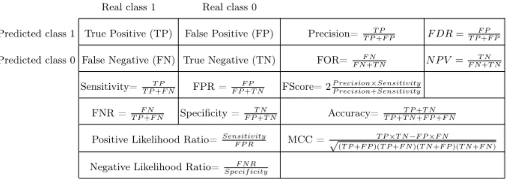
is used to assign classes to new, unlabelled objects in another dataset D that relies on the same features. The true classes of these new objects is known and the performance of the decision tree is related to its ability to assign the correct classes to objects. This performance can be quantified using measures [8]. Some of these measures are combinations of four values:
– True positive (TP), the number of objects belonging to the class 1 that have been assigned the class 1
– False positive (FP), the number of objects belonging to the class 0 that have been assigned the class 1
– False negative (FN), the number of objects belonging to the class 1 that have been assigned the class 0
– True negative (TN), the number of objects belonging to the class 0 that have been assigned the class 0
Some of the performance measures that rely on these four values are presented in Table 1. Let m(D) denote the value of the measure m quantifying the perfor-mance of the decision tree when assigning classes to the objects of the dataset D. Let Dif denote the state of dataset D after a number i of random permutations of the values of the feature f . The impact of the feature f on the value of the measure m for the decision tree, denoted Impact(f, m), is defined as the average variation of the value of m when the values that the feature takes in the dataset are randomly permuted, i.e., for a large enough number k of permutations,
Impact(f, m) ≈ k X i=1 m(Dif) − m(D) k
A negative impact means that the decision tree performs worse when the feature is disturbed and thus that the decision tree relies on values of the features to achieve its performance as quantified by the measure. As impacts are numerical values, features can be ranked according to their impacts on the value of a measure.
Real class 1 Real class 0 Predicted class 1
Predicted class 0
True Positive (TP) False Positive (FP) Precision= T P
T P +F P F DR = F P T P +F P
False Negative (FN) True Negative (TN) FOR= F N
F N +T N N P V = T N F N +T N Sensitivity= T P T P +F N FPR = F P F P +T N FScore= 2 P recision×Sensitivity P recision+Sensitivity FNR = F N T P +F N Specificity = T N F P +T N Accuracy= T P +T N T P +T N +F P +F N
Positive Likelihood Ratio=SensitivityF P R MCC =
T P ×T N −F P ×F N
√
(T P +F P )(T P +F N )(T N +F P )(T N +F N )
Negative Likelihood Ratio= F N R Specif icity
Table 1. Some of the measures of a model’s performance based on the four values TP, FP, FN and TN.
Continuing our example, we would like to know which features are “the best” for the decision tree’s performance. As the rankings of the features induced by different performance measures are not necessarily identical, identifying “the best” features can be expressed as a multicriteria decision problem in which the alternatives are the features and the criteria are the rankings induced by the performance measures. In this example, we suppose that five measures are con-sidered so the multicriteria decision problem involves five criteria C = {Accuracy, Sensitivity, Specif icity, F Score, P recision} (later identified as c1 to c5) and
five alternatives A = {a1, a2, a3, a4, a5}. We further suppose that the impacts of
the features on the model’s score for the five measures translate into the following rankings:
c1= Accuracy : a1 a3 a4 a2 a5
c2= Sensitivity : a2 a3 a1 a4 a5
c3= Specif icity : a1 a4 a3 a2 a5
c4= F Score : a2 a3 a1 a5 a4
c5= P recision : a2 a1 a4 a3 a5
Using the Pareto front as a multicriteria decision method, we obtain that three alternatives (features) are best, i.e. P areto(C, A) = {a1, a2, a3}. The
alter-natives a4and a5are Pareto-dominated by a1. It follows that the features a1, a2
and a3are those that have the highest impact on the decision tree’s performance.
In the next two sections, we develop our approach for explaining the presence of these alternatives on the Pareto front.
3.2 Identifying the Criteria Responsible for the Decisions
In order to explain why an alternative a is considered as the “best” in a multi-criteria decision problem, we first have to identify the minimal criterion sets for which a is on the Pareto front. In other words, we are looking for an algorithm to compute the criterion sets C1such that a ∈ P areto(C1, A) and, for all C2⊂ C1,
a 6∈ P areto(C2, A). As computing the Pareto front of a criterion set is
computa-tionally expensive, we have to navigate the powerset of criteria as efficiently as possible.
Let F = {A ⊆ A | ∃C ⊆ C, A = P areto(C, A)} be the family of alternative sets A for which there exists a criterion set C such that P areto(C, A) = A. In our running example, F = {{a1, a2, a3},{a1, a2},{a1},{a2},∅}. Multiple criterion
sets can have the same Pareto front. Hence, the P areto(·, A) function induces equivalence classes on the powerset of criteria: two criterion sets C1 and C2
are equivalent if and only if P areto(C1, A) = P areto(C2, A). For an alternative
set A ∈ F , we use Crit(A) to denote the family of criterion sets C such that P areto(C, A) = A. In other words, Crit(A) is the equivalence class of criterion sets for which A is the Pareto front. In our running example, Crit({a1, a2}) =
{{c1, c5}, {c3, c5}, {c1, c3, c5}}. We want to compute the minimal elements of each
equivalence class.
To do this, let us define the interior operator i : 2C 7→ 2C that, to a
crite-rion set C, associates i(C), the lectically smallest inclusion-minimal subset of C for which P areto(C, A) = P areto(i(C), A). The images of i are the minimal elements of each equivalence class. In our running example, the images of i are {c1, c2}, {c1, c4}, {c2, c3}, {c3, c4} that have {a1, a2, a3} as Pareto front, {c1, c5},
{c3, c5} that have {a1, a2} as Pareto front, {c1}, {c3} that have {a1} as Pareto
front, {c2}, {c4}, {c5} that have {a2} as Pareto front and ∅ that has an empty
Pareto front.
Algorithm 1 is used to compute i(C). It performs a depth-first search of the powerset of criteria, starting from C, to find the lectically smallest inclusion-minimal criterion set that has the same Pareto front as C. The algorithm at-tempts to remove the criteria in the set one by one in increasing order. A criterion
is removed if its removal does not change the Pareto front. As the criteria are removed in increasing order, it ensures the lectically smallest subset of C that has the same Pareto front is reached.
Algorithm 1: Algorithm for computing i(C).
Input: Criterion set C, Alternative set A and a total order on C Output: i(C)
1 begin
2 P ← P areto(C, A);
3 R ← C;
4 forall x ∈ C in increasing order do
5 if P == P areto(C \ {x}, A) then 6 R ← R \ {x};
7 return R
As interior and closure operators are dual, computing the images of i can be treated as the problem of computing closed sets. Algorithm 2 computes all the images of i(·) with a Next Closure-like approach [5, 1]. Note that, for a criterion set C ⊆ C, we useC to denote C \ C.
Algorithm 2: Algorithm for computing all the images of i(·).
Input: Criterion set C, Alternative set A and a total order on C Output: The set of images of i(·)
1 begin
2 I ← {∅}; 3 C = i(∅);
4 while C 6= C do
5 I ← I ∪ {C};
6 forall x 6∈ C in decreasing order do 7 D ← i({c ∈ C | c ≤ x} ∪ {x});
8 if x == min(C∆D) then
9 C ← D;
10 return I
The minimal criterion sets for which an alternative a is on the Pareto front are the minimal elements of the equivalence classes Crit(A) with A minimal such that a ∈ A. Therefore, not all the images of i are useful. We use
to denote the minimal sets of criteria for which the alternative a belongs to the Pareto front.
In our running example, the only element of F containing the alternative a3
is {a1, a2, a3}. The images of i in Crit({a1, a2, a3}) are {c1, c2}, {c1, c4}, {c2, c3},
{c3, c4}. These are the minimal criteria sets for which a3appears on the Pareto
front. Overall, we have M (a1) = {{c1},{c3}}
M (a2) = {{c2},{c4},{c5}}
M (a3) = {{c1, c2},{c1, c4},{c2, c3},{c3, c4}}
Note that alternatives a1 and a2 are on the Pareto front because of single
criteria while a3requires multiple criteria to be on the Pareto front.
3.3 Explaining the Decisions
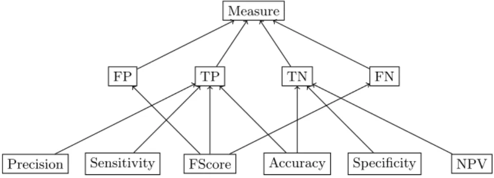
Once we have identified the minimal sets of criteria for which an alternative is on the Pareto front, we interpret them using background knowledge. This background knowledge takes the form of a set T of terms and a set B of impli-cations between terms. In our running example, we arbitrarily choose to use as terms the names of the performance measures as well as T P , F P , T N , F N and M easure. The name of a measure implies the names of the values used in the measure’s numerator. Hence, {Sensitivity} → {T P } because the T P value is used in Sensitivity’s numerator. Similarly, {F Score} → {T P, F N, F P } because both P recision = T P +F NT P and Sensitivity = T P +F PT P are used in F Score’s nu-merator. Additionally, all the terms imply M easure because both measures and values used in measures are measures. This background knowledge induces the partial order on the set of terms depicted in Fig. 1.
Measure
TP FN
FP TN
Sensitivity FScore Accuracy Specificity NPV Precision
Fig. 1. Example of background knowledge as a partially ordered set of terms.
Considering this partial ordering as an interpretation domain, we assign to a criterion ci an interpretation by means of a criterion interpretation function
Ic(·) : C 7→ 2T that maps ci to a subset of T closed under the logical closure
by the implications of B. In our running example, Ic(ci) is the logical closure
of the name of the measure associated with the criterion ci. Hence, since c2 =
Sensitivity, Ic(c2) = B({Sensitivity}) = {Sensitivity, T P, M easure}. Overall,
in our running example:
Ic(c1) = B({Accuracy}) = {Accuracy, T P, T N, M easure}
Ic(c2) = B({Sensitivity}) = {Sensitivity, T P, M easure}
Ic(c3) = B({Specif icity}) = {Specif icity, T N, M easure}
Ic(c4) = B({F Score}) = {F Score, F P, T P, F N, M easure}
Ic(c5) = B({P recision}) = {P recision, T P, M easure}
We then use the interpretations of criteria to explain the reason why an alternative is on the Pareto front. In our running example, a1 appears on the
Pareto front as soon as either c1or c3is taken into account. As c1represents the
impact of features on the accuracy score of the decision tree, we can say that a1
is on the Pareto front because it is particularly good for accuracy. Similarly, as c3represents the impact of features on the specificity score of the decision tree,
a1 is also good for specificity. The alternative a3 only starts appearing on the
Pareto front when two criteria are taken into account simultaneously, such as c1
and c2. In this situation, we can only say that a3 is good for the commonalities
of c1 and c2. As c2 represents the impact of features on the sensitivity score of
the model, according to our background knowledge, we can say that a3 is good
for measures that use the T P value. Formally, we define the interpretation of an alternative by means of the alternative interpretation function Ia(·) : A 7→ 2T
that maps an alternative ai to Ia(ai) =SC∈M (ai)Tcj∈CIc(cj), i.e. a subset of
T closed under the logical closure by the implications of B.
Finally, we use formal concept analysis to classify the alternatives according to their interpretations and present the explanation of the presence of alterna-tives on the Pareto front in the form of a concept lattice. The interpretation of an alternative provides its description, which gives rise to the formal context (P areto(C, A), T , Ra) in which (ai, t) ∈ Ra if and only if t ∈ Ia(ai). In our
run-ning example, this formal context is the one depicted in Table 2. In the concepts of this context, the extents are sets of alternatives on the Pareto front of the multicriteria decision problem and the intents are interpretations of these alter-natives that explain the reason why these alteralter-natives are on the Pareto front. Figure 2 presents the concept lattice of our running example. For legibility rea-sons, only the most specific terms, according to the background knowledge, are displayed.
From this concept lattice, we learn that a2 is among the best features for
the decision tree’s performance because it is the best for the Sensitivity, FScore and Precision scores while a1is the best for the Accuracy and Specificity scores.
The feature a3 is not the best for any particular measure’s score but is a good
Accuracy Sensitivity Specificity FScore Precision TP FN FP TN Measure
a1 × × × × ×
a2 × × × × × × ×
a3 × ×
Table 2. Formal context ({a1, a2, a3}, T , Ra) of our running example.
(∅,{Accuracy, Sensitivity, Specificity, FScore, Prediction})
({a1},{Accuracy, Specificity})
({a2},{Sensitivity, FScore, Precision})
({a1, a2, a3},{TP})
Fig. 2. Concept lattice presenting sets of alternatives from our running example to-gether with an explanation of their presence on the Pareto front.
4
Experimental Example
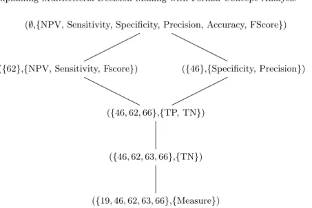
The Lymphography dataset is a public dataset available on the UCI machine learning repository1. In its binarised version, it contains 148 objects described by 68 binary attributes identified by numbers. We used it to train a Naive Bayes classifier and to rank the features according to their impacts on six measures: Sensitivity, Specificity, Precision, Accuracy, Fscore and NPV. Identifying the best features for the Naive Bayes classifier’s performance is a multicriteria decision problem in the same manner as our running example. Our method was applied to this multicriteria decision problem and produced the concept lattice depicted in Fig. 3.
In this concept lattice, we see that five features are the best for the model. The feature 62 is the best for the NPV, Sensitivity and FScore measures. The feature 46 is the best for the Specificity and Precision measures. The feature 66 represents a good compromise for measures that use the TP or TN value. The feature 63 is a good compromise for measures that use the TN values. Finally, the feature 19 is a good compromise for measures in general. This explanation can, for example, be used in a feature selection [7] process to optimise the performance of classifiers.
5
Conclusion
The proposed approach provides an explanation of the output of multicriteria decision methods. The approach requires the presence of an alternative in the
1
(∅,{NPV, Sensitivity, Specificity, Precision, Accuracy, FScore}) ({46},{Specificity, Precision}) ({62},{NPV, Sensitivity, Fscore}) ({46, 62, 66},{TP, TN}) ({46, 62, 63, 66},{TN}) ({19, 46, 62, 63, 66},{Measure})
Fig. 3. Concept lattice presenting an explanation of the best features from the binarised Lymphography dataset according to a naive Bayes classifier.
solutions returned by the decision method to be monotonic w.r.t. the set of considered criteria. Decisions methods that satisfy this property include, among others, the Pareto front and all methods that return ideals of the set of alterna-tives partially ordered by the Pareto dominance relation.
The explanations that are created rely on background knowledge of the cri-teria. This allows the approach to be applied to any problem in which rankings of elements are produced by processes that are understood in some way.
Acknowledgement
This work was supported partly by the french PIA project « Lorraine Université d’Excellence », reference ANR-15-IDEX-04-LUE.
References
1. Borchmann, D.: A generalized next-closure algorithm - enumerating semilattice ele-ments from a generating set. In: Proceedings of The Ninth International Conference on Concept Lattices and Their Applications, Fuengirola (Málaga), Spain, October 11-14, 2012. pp. 9–20 (2012)
2. Bouyssou, D., Dubois, D., Prade, H., Pirlot, M.: Decision Making Process: Concepts and Methods. John Wiley & Sons (2013)
3. Bouyssou, D., Marchant, T., Pirlot, M., Tsoukias, A., Vincke, P.: Evaluation and Decision Models with Multiple Criteria: Stepping Stones for the Analyst, vol. 86. Springer Science & Business Media (2006)
4. Distel, F., Sertkaya, B.: On the complexity of enumerating pseudo-intents. Discrete Applied Mathematics 159(6), 450–466 (2011)
5. Ganter, B., Wille, R.: Formal Concept Analysis: Mathematical Foundations. Springer - Verlag (1999)
6. Ryssel, U., Distel, F., Borchmann, D.: Fast algorithms for implication bases and attribute exploration using proper premises. Annals of Mathematics and Artificial Intelligence 70(1-2), 25–53 (2014)
7. Saeys, Y., Inza, I., Larrañaga, P.: A review of feature selection techniques in bioin-formatics. Bioinformatics 23(19), 2507–2517 (2007)
8. Sokolova, M., Lapalme, G.: A systematic analysis of performance measures for clas-sification tasks. Information Processing & Management 45(4), 427–437 (2009)