Benchmarking Algorithms from the platypus Framework on the Biobjective bbob-biobj Testbed

(1)

HAL Id: hal-02171136

https://hal.inria.fr/hal-02171136

Submitted on 2 Jul 2019

HAL is a multi-disciplinary open access

archive for the deposit and dissemination of

sci-entific research documents, whether they are

pub-lished or not. The documents may come from

teaching and research institutions in France or

abroad, or from public or private research centers.

L’archive ouverte pluridisciplinaire HAL, est

destinée au dépôt et à la diffusion de documents

scientifiques de niveau recherche, publiés ou non,

émanant des établissements d’enseignement et de

recherche français ou étrangers, des laboratoires

publics ou privés.

Benchmarking Algorithms from the platypus Framework

on the Biobjective bbob-biobj Testbed

Dimo Brockhoff, Tea Tušar

To cite this version:

Dimo Brockhoff, Tea Tušar. Benchmarking Algorithms from the platypus Framework on the

Biob-jective bbob-biobj Testbed. GECCO 2019 - The Genetic and Evolutionary Computation Conference,

Jul 2019, Prague, Czech Republic. �10.1145/3319619.3326896�. �hal-02171136�

(2)

Benchmarking Algorithms from the platypus Framework on the

Biobjective bbob-biobj Testbed

Dimo Brockhoﬀ

Inria and CMAP, Ecole Polytechnique Institut Polytechnique de Paris

Palaiseau, France dimo.brockhoﬀ@inria.fr

Tea Tuˇsar

Department of Intelligent Systems Joˇzef Stefan Institute

Ljubljana, Slovenia [email protected]

ABSTRACT

One of the main goals of the COCO platform is to produce, col-lect, and make available benchmarking performance data sets of optimization algorithms and, more concretely, algorithm imple-mentations. For the recently proposed biobjective bbob-biobj test suite, less than 20 algorithms have been benchmarked so far but many more are available to the public. We therefore aim in this paper to benchmark several available multiobjective optimization algorithms on the bbob-biobj test suite and discuss their perfor-mance. We focus here on algorithms implemented in the platypus framework (in Python) whose main advantage is its ease of use without the need to set up many algorithm parameters.

CCS CONCEPTS

•Computing methodologies → Continuous space search;

KEYWORDS

Benchmarking, Black-box optimization, Bi-objective optimization

ACM Reference format:

Dimo Brockhoﬀ and Tea Tuˇsar. 2019. Benchmarking Algorithms from the platypusFramework on the Biobjective bbob-biobj Testbed. In Proceed-ings of Genetic and Evolutionary Computation Conference Companion, Prague, Czech Republic, July 13–17, 2019 (GECCO ’19 Companion),7pages. DOI: 10.1145/3319619.3326896

1 INTRODUCTION

Among the most diﬃcult tasks when solving a black-box optimiza-tion problem in practice is to choose an appropriate optimizaoptimiza-tion algorithm from the vast amount of available ones. Making such a decision based on experimental data from numerical benchmarking experiments is the most viable alternative. The Comparing

Contin-uous Optimizers platform (COCO, [7],github.com/numbbo/coco/)

assists in this task by automatizing the benchmarking experiments and, more importantly, by freely providing the data of many such experiments to the public.

This is an author version of the GECCO Companion 2019 workshop paper published by Springer Verlag. The final publication is available at www.springerlink.com. Permission to make digital or hard copies of all or part of this work for personal or classroom use is granted without fee provided that copies are not made or distributed for profit or commercial advantage and that copies bear this notice and the full citation on the first page. Copyrights for components of this work owned by others than the author(s) must be honored. Abstracting with credit is permitted. To copy otherwise, or republish, to post on servers or to redistribute to lists, requires prior specific permission and/or a fee. Request permissions from [email protected].

GECCO ’19 Companion, Prague, Czech Republic

DOI: 10.1145/3319619.3326896

Since 2016, COCO also oﬀers a biobjective benchmark suite

(called bbob-biobj, [12]) with 55 objective functions that are

com-posed of the original single-objective bbob functions. Compared to the 190+ algorithm data sets for the original bbob suite, only few algorithms have been compared on the bbob-biobj suite so far— despite the huge amount of available multiobjective optimization algorithms in the literature.

In this paper, we contribute to COCO’s bbob-biobj data set by running experiments with several multiobjective optimization

algo-rithms from the platypus library (in Python).1These algorithms

are well-known in the evolutionary multiobjective optimization community and have performed well in several previous algorithm comparisons. The platypus library already provides default values for the algorithms’ internal parameters, making it easy to use for practitioners. The next section gives more details on the algorithms compared here.

2 ALGORITHMS IN THE COMPARISON

In the following, we compare the platypus implementation of the

algorithms NSGA-II [5], IBEA [14], MOEA/D [13], SPEA2 [15] and

GDE3 [10], as well as of the recently proposed NSGA-III [4]. It will

be especially interesting to see how the platypus implementation of NSGA-II compares with the one in Matlab from the gamultiobj library that has been benchmarked on the bbob-biobj suite before

[1]. We denote the latter algorithm as NSGA-II-MATLAB in the

remainder of the paper.

Not contained in our comparison are the lesser known algorithms OMOPSO, SMPSO, and EpsMOEA as well as the CMAES algorithm from platypus for which preliminary experiments with the default setup showed signiﬁcantly worse results than the available

UP-MO-CMA-ES data set of [9].

3 EXPERIMENTAL PROCEDURE

All algorithm implementations have been taken from the platypus

framework (https://github.com/Project-Platypus/Platypus) with the

version “4 - beta” as of November 20172.

Let n denote the problem dimension. GDE3, IBEA, and NSGA-II

have been run for 105n_{function evaluations, SPEA2 and NSGA-III}

for 104n_{function evaluations (due to slower internal computations).}

Note here that the experimental setup of COCO does not impose a concrete number of function evaluations and that COCO’s target-based performance assessment allows naturally to compare data

1_{The source code is available from}_{https://github.com/Project-Platypus/Platypus}_. 2_{Until then, only a callback functionality was added and the documentation was}

updated such that the current platypus version at the time of the paper submission shall be the same as the version used for the experiments.

(3)

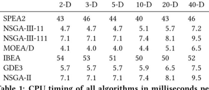
GECCO ’19 Companion, July 13–17, 2019, Prague, Czech Republic Dimo Brockhoﬀ 2-D 3-D 5-D 10-D 20-D 40-D SPEA2 43 46 44 40 43 46 NSGA-III-11 4.7 4.7 4.7 5.1 5.7 7.2 NSGA-III-111 7.1 7.1 7.1 7.4 8.1 9.5 MOEA/D 4.1 4.0 4.0 4.4 5.1 6.5 IBEA 54 53 51 50 50 52 GDE3 5.7 5.7 5.7 5.9 6.5 7.5 NSGA-II 7.1 7.1 7.1 7.4 8.1 9.5

Table 1: CPU timing of all algorithms in milliseconds per function evaluation for the standard bbob-biobj dimensions 2 to 40.

from experiments that have been run with diﬀerent numbers of function evaluations.

For NSGA-III, we have run two versions, one with 11 and one with 111 reference points, denoted by N-III-11 and N-III-111 in the

following.3Besides this one parameter, all algorithms have been

run with platypus’ standard settings and a population size of 100 in particular, except for the initialization. In our experiments, we

ﬁrst evaluate the search space origin[0, . . . ,0] ∈ Rnfollowing the

recommendation in the (Python) example experiment of COCO and then initialize the actual platypus algorithm by sampling the

ﬁrst population uniformly at random within[−5,5]n, according

to the bbob-biobj test suite which guarantees that the extreme solutions of the Pareto front are contained in this box. For NSGA-II, we also consider other initializations later when comparing it with

the Matlab version from [1].

4 CPU TIMING

In order to evaluate the CPU timing of the algorithms, we have collected the runtimes per function evaluation of all experiments

according to [8] for a budget of 1000n on the ﬁrst three instances.

The Python code was run on a Linux machine with 64 Intel(R) Xeon(R) CPU E5-2683 v4 @ 2.10GHz processors but with other load on the machine. The time per function evaluation for dimensions 2,

3, 5, 10, 20, and 40 is given in Table1.

We can observe that there are two groups of algorithms in terms of cpu timing: SPEA2 and IBEA need about 5–10 times as much time per function evaluation than the other tested platypus algo-rithms. Over dimension, the cpu timing results are rather stable with slightly increased times in dimensions 20 and 40 for the latter (faster) group of algorithms.

5 RESULTS

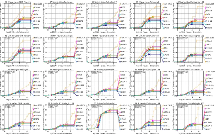
Results from experiments according to [8], [6] and [3] on the

benchmark functions given in [12] are presented in Figures1,2,

3and4. For more details, in particular the tabular data, we

re-fer to the supplementary material athttp://randopt.gforge.inria.fr/

ppdata-archive/2019-platypus/. The experiments were performed

with COCO [7], version 2.0 or 2.2.x depending on the algorithm.

The plots were produced with COCO version 2.3.1 that explicitly

3_{Note that platypus does not provide a default value here such that we run two variants}

with (arbitrary) numbers of reference points in the order of magnitude of the default population size of 100.

turns of simulated restarts for the empirical runtime distribution plots (as indicated by always ﬂat curves after the cross).

The average runtime (aRT), used in the tables, depends on a

given quality indicator value, Itarget= Iref+ ∆IHVCOCO, and is

com-puted over all relevant trials as the number of function evaluations executed during each trial while the best indicator value did not

reach Itarget, summed over all trials and divided by the number of

trials that actually reached Itarget[8,11]. Statistical signiﬁcance

is tested with the rank-sum test for a given target Itarget using,

for each trial, either the number of needed function evaluations

to reach Itarget(inverted and multiplied by−1), or, if the target

was not reached, the best ∆IHVCOCO-value achieved, measured only

up to the smallest number of overall function evaluations for any unsuccessful trial under consideration.

From the graphs and tables, the following main observations can be made.

Overall performance. Surprisingly, the platypus algorithms are all relatively similar in performance, in particular when compared to the already existing data sets of COCO, which are more diverse, see

for examplehttp://coco.gforge.inria.fr/ppdata-archive/bbob-biobj/

2016-all/. The platypus algorithms included in this comparison can be found in the middle performance range similar to an algo-rithm like SMS-EMOA, but are deﬁnitely outperformed in the larger dimensions by the hybrid HMO-CMA-ES and for larger budgets also by RM-MEDA and UP-MO-CMA-ES.

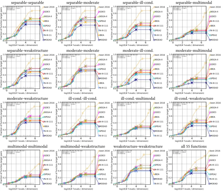
The few trends among the platypus algorithms that can be reported is that MOEA/D falls short after some time and that NSGA-III with 11 reference vectors is outperforming the other algorithms around 100n function evaluations (the improvement over the second-best algorithm, however, is only about a factor of 1.5–2). Exceptions where MOEA/D is not falling behind in

dimen-sion 5–20 are the following 26 of the 55 bbob-biobj functions: F1

(where for large budgets in dimension 20, MOEA/D is here even

the best algorithm), F5–F8, F10, F11, F20, F21, F26(not in dimension

20), F28, F33, F35–F37, F41–F43, F45–F47, F49, F50, F52, F53and F55.

Similar observations can be made in lower dimensions where the diﬀerences, however, are smaller.

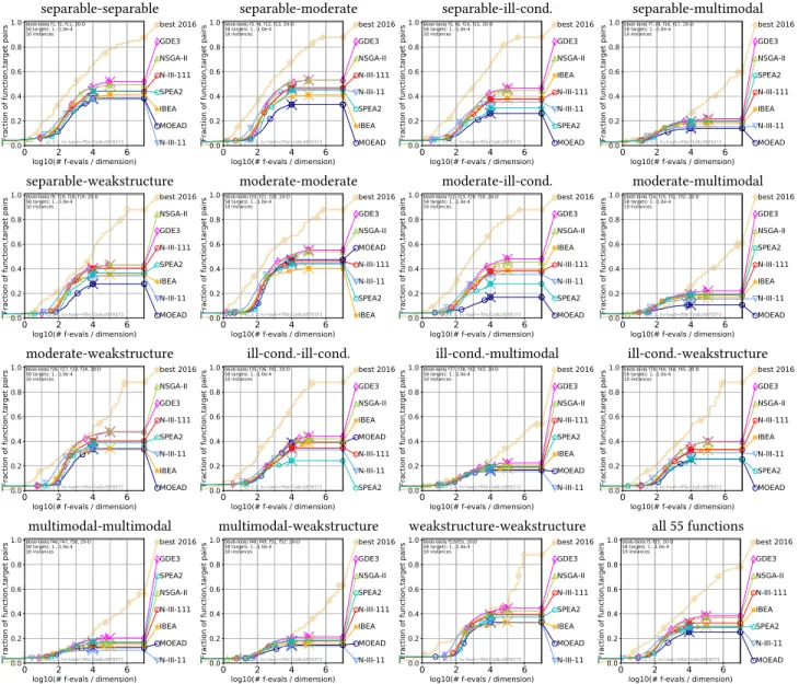
Over all functions, in particular in the higher dimensions, GDE3 is the best algorithm for the larger budgets, followed almost imme-diately by the performance of NSGA-II. In the lower dimension and for larger budgets, it is NSGA-II that is outperforming GDE3. This good performance of GDE3 and NSGA-II can be mostly attributed to problems where the objectives come from the separable, mod-erate, and ill-conditioned function classes of the original bbob test suite—in the higher dimensions, in particular in 20-D, GDE3 and NSGA-II are often the best algorithms among the tested ones for a large range of budgets.

6 COMPARISON BETWEEN NSGA-II

IMPLEMENTATIONS

Benchmarking algorithms is a non-trivial task, especially when it comes to different implementations of one and the same (theoretical) algorithm. Here, we would like to make the point that, in practice, we can only compare algorithm implementations and that they may differ quite significantly.

(4)

0 2 4 6

log10(# f-evals / dimension) 0.0 0.2 0.4 0.6 0.8 1.0

Fraction of function,target pairs N-III-11 SPEA2 IBEA N-III-111 NSGA-II MOEAD GDE3 best 2016 bbob-biobj f1, 10-D 58 targets: 1..-1.0e-4 10 instances v2.3.1, hv-hash=ff0e71e8cd978373 1 Sphere/Sphere 0 2 4 6

Fraction of function,target pairs MOEAD N-III-11 IBEA N-III-111 SPEA2 NSGA-II GDE3 best 2016 bbob-biobj f2, 10-D 58 targets: 1..-1.0e-4 10 instances v2.3.1, hv-hash=ff0e71e8cd978373 2 Sphere/sep. Ellipsoid 0 2 4 6

Fraction of function,target pairs MOEAD N-III-11 N-III-111 SPEA2 IBEA NSGA-II GDE3 best 2016 bbob-biobj f3, 10-D 58 targets: 1..-1.0e-4 10 instances v2.3.1, hv-hash=ff0e71e8cd978373 3 Sphere/Attr. sector 0 2 4 6

Fraction of function,target pairs MOEAD IBEA N-III-11 N-III-111 SPEA2 NSGA-II GDE3 best 2016 bbob-biobj f4, 10-D 58 targets: 1..-1.0e-4 10 instances v2.3.1, hv-hash=ff0e71e8cd978373 4 Sphere/Rosenbrock 0 2 4 6

Fraction of function,target pairs SPEA2 MOEAD N-III-11 N-III-111 NSGA-II GDE3 IBEA best 2016 bbob-biobj f5, 10-D 58 targets: 1..-1.0e-4 10 instances v2.3.1, hv-hash=ff0e71e8cd978373 5 Sphere/Sharp ridge 0 2 4 6

Fraction of function,target pairs N-III-11 IBEA SPEA2 N-III-111 MOEAD NSGA-II GDE3 best 2016 bbob-biobj f6, 10-D 58 targets: 1..-1.0e-4 10 instances v2.3.1, hv-hash=ff0e71e8cd978373 6 Sphere/Different Powers 0 2 4 6

Fraction of function,target pairs N-III-11 MOEAD IBEA SPEA2 N-III-111 NSGA-II GDE3 best 2016 bbob-biobj f7, 10-D 58 targets: 1..-1.0e-4 10 instances v2.3.1, hv-hash=ff0e71e8cd978373 7 Sphere/Rastrigin 0 2 4 6

Fraction of function,target pairs N-III-11 MOEAD IBEA SPEA2 NSGA-II N-III-111 GDE3 best 2016 bbob-biobj f8, 10-D 58 targets: 1..-1.0e-4 10 instances v2.3.1, hv-hash=ff0e71e8cd978373 8 Sphere/Schaffer F7 0 2 4 6

Fraction of function,target pairs MOEAD N-III-11 IBEA N-III-111 SPEA2 NSGA-II GDE3 best 2016 bbob-biobj f9, 10-D 58 targets: 1..-1.0e-4 10 instances v2.3.1, hv-hash=ff0e71e8cd978373 9 Sphere/Schwefel 0 2 4 6

Fraction of function,target pairs N-III-11 IBEA MOEAD SPEA2 GDE3 N-III-111 NSGA-II best 2016 bbob-biobj f10, 10-D 58 targets: 1..-1.0e-4 10 instances v2.3.1, hv-hash=ff0e71e8cd978373 10 Sphere/Gallagher 101 0 2 4 6

Fraction of function,target pairs N-III-11 N-III-111 SPEA2 MOEAD NSGA-II GDE3 IBEA best 2016 bbob-biobj f11, 10-D 58 targets: 1..-1.0e-4 10 instances v2.3.1, hv-hash=ff0e71e8cd978373

11 sep. Ellipsoid/sep. Elli.

0 2 4 6

Fraction of function,target pairs IBEA MOEAD N-III-11 N-III-111 SPEA2 GDE3 NSGA-II best 2016 bbob-biobj f12, 10-D 58 targets: 1..-1.0e-4 10 instances v2.3.1, hv-hash=ff0e71e8cd978373

12 sep. Ellipsoid/Attr. sector

0 2 4 6

Fraction of function,target pairs MOEAD IBEA N-III-111 N-III-11 SPEA2 GDE3 NSGA-II best 2016 bbob-biobj f13, 10-D 58 targets: 1..-1.0e-4 10 instances v2.3.1, hv-hash=ff0e71e8cd978373 13 sep. Ellipsoid/Rosenbrock 0 2 4 6

Fraction of function,target pairs MOEAD SPEA2 N-III-11 N-III-111 IBEA GDE3 NSGA-II best 2016 bbob-biobj f14, 10-D 58 targets: 1..-1.0e-4 10 instances v2.3.1, hv-hash=ff0e71e8cd978373

14 sep. Ellipsoid/Sharp ridge

0 2 4 6

Fraction of function,target pairs MOEAD IBEA N-III-11 N-III-111 SPEA2 NSGA-II GDE3 best 2016 bbob-biobj f15, 10-D 58 targets: 1..-1.0e-4 10 instances v2.3.1, hv-hash=ff0e71e8cd978373

15 sep. Ellipsoid/Diff. Powers

0 2 4 6

Fraction of function,target pairs MOEAD N-III-11 IBEA SPEA2 N-III-111 NSGA-II GDE3 best 2016 bbob-biobj f16, 10-D 58 targets: 1..-1.0e-4 10 instances v2.3.1, hv-hash=ff0e71e8cd978373 16 sep. Ellipsoid/Rastrigin 0 2 4 6

Fraction of function,target pairs MOEAD N-III-11 IBEA NSGA-II N-III-111 SPEA2 GDE3 best 2016 bbob-biobj f17, 10-D 58 targets: 1..-1.0e-4 10 instances v2.3.1, hv-hash=ff0e71e8cd978373 17 sep. Ellipsoid/Schaffer F7 0 2 4 6

Fraction of function,target pairs MOEAD N-III-11 IBEA SPEA2 N-III-111 NSGA-II GDE3 best 2016 bbob-biobj f18, 10-D 58 targets: 1..-1.0e-4 10 instances v2.3.1, hv-hash=ff0e71e8cd978373 18 sep. Ellipsoid/Schwefel 0 2 4 6

Fraction of function,target pairs MOEAD N-III-11 IBEA N-III-111 SPEA2 GDE3 NSGA-II best 2016 bbob-biobj f19, 10-D 58 targets: 1..-1.0e-4 10 instances v2.3.1, hv-hash=ff0e71e8cd978373 19 sep. Elli./Gallagher 101 0 2 4 6

Fraction of function,target pairs IBEA MOEAD N-III-11 SPEA2 N-III-111 NSGA-II GDE3 best 2016 bbob-biobj f20, 10-D 58 targets: 1..-1.0e-4 10 instances v2.3.1, hv-hash=ff0e71e8cd978373

20 Attr. sector/Attr. sector

0 2 4 6

Fraction of function,target pairs IBEA N-III-11 MOEAD N-III-111 SPEA2 NSGA-II GDE3 best 2016 bbob-biobj f21, 10-D 58 targets: 1..-1.0e-4 10 instances v2.3.1, hv-hash=ff0e71e8cd978373 21 Attr. sector/Rosenbrock 0 2 4 6

Fraction of function,target pairs MOEAD SPEA2 N-III-11 N-III-111 GDE3 NSGA-II IBEA best 2016 bbob-biobj f22, 10-D 58 targets: 1..-1.0e-4 10 instances v2.3.1, hv-hash=ff0e71e8cd978373

22 Attr. sector/Sharp ridge

0 2 4 6

Fraction of function,target pairs MOEAD N-III-11 SPEA2 N-III-111 IBEA NSGA-II GDE3 best 2016 bbob-biobj f23, 10-D 58 targets: 1..-1.0e-4 10 instances v2.3.1, hv-hash=ff0e71e8cd978373

23 Attr. sector/Diff. Powers

0 2 4 6

Fraction of function,target pairs MOEAD N-III-11 IBEA SPEA2 N-III-111 NSGA-II GDE3 best 2016 bbob-biobj f24, 10-D 58 targets: 1..-1.0e-4 10 instances v2.3.1, hv-hash=ff0e71e8cd978373 24 Attr. sector/Rastrigin 0 2 4 6

Fraction of function,target pairs MOEAD N-III-11 IBEA N-III-111 SPEA2 NSGA-II GDE3 best 2016 bbob-biobj f25, 10-D 58 targets: 1..-1.0e-4 10 instances v2.3.1, hv-hash=ff0e71e8cd978373 25 Attr. sector/Schaffer F7 0 2 4 6

Fraction of function,target pairs IBEA N-III-11 MOEAD N-III-111 SPEA2 NSGA-II GDE3 best 2016 bbob-biobj f26, 10-D 58 targets: 1..-1.0e-4 10 instances v2.3.1, hv-hash=ff0e71e8cd978373 26 Attr. sector/Schwefel 0 2 4 6

Fraction of function,target pairs MOEAD N-III-11 IBEA N-III-111 NSGA-II SPEA2 GDE3 best 2016 bbob-biobj f27, 10-D 58 targets: 1..-1.0e-4 10 instances v2.3.1, hv-hash=ff0e71e8cd978373 27 Attr. sector/Gallagher 101 0 2 4 6

Fraction of function,target pairs IBEA SPEA2 N-III-11 N-III-111 MOEAD GDE3 NSGA-II best 2016 bbob-biobj f28, 10-D 58 targets: 1..-1.0e-4 10 instances v2.3.1, hv-hash=ff0e71e8cd978373 28 Rosenbrock/Rosenbrock 0 2 4 6

Fraction of function,target pairs MOEAD SPEA2 N-III-111 IBEA N-III-11 GDE3 NSGA-II best 2016 bbob-biobj f29, 10-D 58 targets: 1..-1.0e-4 10 instances v2.3.1, hv-hash=ff0e71e8cd978373 29 Rosenbrock/Sharp ridge 0 2 4 6

Fraction of function,target pairs MOEAD IBEA N-III-11 SPEA2 N-III-111 NSGA-II GDE3 best 2016 bbob-biobj f30, 10-D 58 targets: 1..-1.0e-4 10 instances v2.3.1, hv-hash=ff0e71e8cd978373 30 Rosenbrock/Diff. Powers 0 2 4 6

Fraction of function,target pairs MOEAD N-III-11 SPEA2 IBEA N-III-111 NSGA-II GDE3 best 2016 bbob-biobj f31, 10-D 58 targets: 1..-1.0e-4 10 instances v2.3.1, hv-hash=ff0e71e8cd978373 31 Rosenbrock/Rastrigin 0 2 4 6

Fraction of function,target pairs MOEAD N-III-11 IBEA N-III-111 SPEA2 NSGA-II GDE3 best 2016 bbob-biobj f32, 10-D 58 targets: 1..-1.0e-4 10 instances v2.3.1, hv-hash=ff0e71e8cd978373 32 Rosenbrock/Schaffer F7 0 2 4 6

Fraction of function,target pairs IBEA N-III-111 MOEAD SPEA2 N-III-11 GDE3 NSGA-II best 2016 bbob-biobj f33, 10-D 58 targets: 1..-1.0e-4 10 instances v2.3.1, hv-hash=ff0e71e8cd978373 33 Rosenbrock/Schwefel 0 2 4 6

Fraction of function,target pairs MOEAD N-III-11 IBEA SPEA2 N-III-111 NSGA-II GDE3 best 2016 bbob-biobj f34, 10-D 58 targets: 1..-1.0e-4 10 instances v2.3.1, hv-hash=ff0e71e8cd978373 34 Rosenbrock/Gallagher 101 0 2 4 6

Fraction of function,target pairs SPEA2 N-III-11 N-III-111 MOEAD GDE3 NSGA-II IBEA best 2016 bbob-biobj f35, 10-D 58 targets: 1..-1.0e-4 10 instances v2.3.1, hv-hash=ff0e71e8cd978373

35 Sharp ridge/Sharp ridge

Figure 1: Empirical cumulative distribution of simulated (bootstrapped) runtimes, measured in

num-ber of objective function evaluations, divided by dimension (FEvals/DIM) for the 58 targets {−10−4

,−10 −4.2 , −10−4.4 ,−10−4.6,−10−4.8,−10−5,0,10−5,10−4.9,10−4.8, . . . ,10−0.1,10 0_{} in dimension 10.}

(5)

GECCO ’19 Companion, July 13–17, 2019, Prague, Czech Republic Dimo Brockhoﬀ

0 2 4 6

Fraction of function,target pairs SPEA2 MOEAD N-III-11 N-III-111 IBEA GDE3 NSGA-II best 2016 bbob-biobj f36, 10-D 58 targets: 1..-1.0e-4 10 instances v2.3.1, hv-hash=ff0e71e8cd978373

36 Sharp ridge/Diff. Powers

0 2 4 6

Fraction of function,target pairs N-III-11 SPEA2 MOEAD N-III-111 IBEA NSGA-II GDE3 best 2016 bbob-biobj f37, 10-D 58 targets: 1..-1.0e-4 10 instances v2.3.1, hv-hash=ff0e71e8cd978373 37 Sharp ridge/Rastrigin 0 2 4 6

Fraction of function,target pairs MOEAD N-III-11 IBEA N-III-111 SPEA2 NSGA-II GDE3 best 2016 bbob-biobj f38, 10-D 58 targets: 1..-1.0e-4 10 instances v2.3.1, hv-hash=ff0e71e8cd978373 38 Sharp ridge/Schaffer F7 0 2 4 6

Fraction of function,target pairs SPEA2 MOEAD N-III-11 N-III-111 NSGA-II GDE3 IBEA best 2016 bbob-biobj f39, 10-D 58 targets: 1..-1.0e-4 10 instances v2.3.1, hv-hash=ff0e71e8cd978373 39 Sharp ridge/Schwefel 0 2 4 6

Fraction of function,target pairs MOEAD SPEA2 N-III-11 N-III-111 IBEA NSGA-II GDE3 best 2016 bbob-biobj f40, 10-D 58 targets: 1..-1.0e-4 10 instances v2.3.1, hv-hash=ff0e71e8cd978373 40 Sharp ridge/Gallagher 101 0 2 4 6

Fraction of function,target pairs SPEA2 N-III-11 IBEA N-III-111 MOEAD NSGA-II GDE3 best 2016 bbob-biobj f41, 10-D 58 targets: 1..-1.0e-4 10 instances v2.3.1, hv-hash=ff0e71e8cd978373

41 Diff. Powers/Diff. Powers

0 2 4 6

Fraction of function,target pairs N-III-11 SPEA2 IBEA MOEAD N-III-111 NSGA-II GDE3 best 2016 bbob-biobj f42, 10-D 58 targets: 1..-1.0e-4 10 instances v2.3.1, hv-hash=ff0e71e8cd978373 42 Diff. Powers/Rastrigin 0 2 4 6

Fraction of function,target pairs MOEAD N-III-11 IBEA N-III-111 SPEA2 NSGA-II GDE3 best 2016 bbob-biobj f43, 10-D 58 targets: 1..-1.0e-4 10 instances v2.3.1, hv-hash=ff0e71e8cd978373 43 Diff. Powers/Schaffer F7 0 2 4 6

Fraction of function,target pairs MOEAD N-III-11 SPEA2 N-III-111 IBEA NSGA-II GDE3 best 2016 bbob-biobj f44, 10-D 58 targets: 1..-1.0e-4 10 instances v2.3.1, hv-hash=ff0e71e8cd978373 44 Diff. Powers/Schwefel 0 2 4 6

Fraction of function,target pairs IBEA N-III-11 SPEA2 N-III-111 MOEAD GDE3 NSGA-II best 2016 bbob-biobj f45, 10-D 58 targets: 1..-1.0e-4 10 instances v2.3.1, hv-hash=ff0e71e8cd978373 45 Diff. Powers/Gallagher 101 0 2 4 6

Fraction of function,target pairs N-III-11 MOEAD IBEA N-III-111 NSGA-II SPEA2 GDE3 best 2016 bbob-biobj f46, 10-D 58 targets: 1..-1.0e-4 10 instances v2.3.1, hv-hash=ff0e71e8cd978373 46 Rastrigin/Rastrigin 0 2 4 6

Fraction of function,target pairs MOEAD N-III-11 IBEA N-III-111 SPEA2 NSGA-II GDE3 best 2016 bbob-biobj f47, 10-D 58 targets: 1..-1.0e-4 10 instances v2.3.1, hv-hash=ff0e71e8cd978373 47 Rastrigin/Schaffer F7 0 2 4 6

Fraction of function,target pairs MOEAD N-III-11 SPEA2 IBEA NSGA-II N-III-111 GDE3 best 2016 bbob-biobj f48, 10-D 58 targets: 1..-1.0e-4 10 instances v2.3.1, hv-hash=ff0e71e8cd978373 48 Rastrigin/Schwefel 0 2 4 6

Fraction of function,target pairs N-III-11 MOEAD SPEA2 IBEA N-III-111 NSGA-II GDE3 best 2016 bbob-biobj f49, 10-D 58 targets: 1..-1.0e-4 10 instances v2.3.1, hv-hash=ff0e71e8cd978373 49 Rastrigin/Gallagher 101 0 2 4 6

Fraction of function,target pairs N-III-11 IBEA MOEAD N-III-111 SPEA2 NSGA-II GDE3 best 2016 bbob-biobj f50, 10-D 58 targets: 1..-1.0e-4 10 instances v2.3.1, hv-hash=ff0e71e8cd978373 50 Schaffer F7/Schaffer F7 0 2 4 6

Fraction of function,target pairs MOEAD N-III-11 IBEA SPEA2 N-III-111 NSGA-II GDE3 best 2016 bbob-biobj f51, 10-D 58 targets: 1..-1.0e-4 10 instances v2.3.1, hv-hash=ff0e71e8cd978373 51 Schaffer F7/Schwefel 0 2 4 6

Fraction of function,target pairs N-III-11 MOEAD SPEA2 IBEA N-III-111 NSGA-II GDE3 best 2016 bbob-biobj f52, 10-D 58 targets: 1..-1.0e-4 10 instances v2.3.1, hv-hash=ff0e71e8cd978373 52 Schaffer F7/Gallagh. 101 0 2 4 6

Fraction of function,target pairs N-III-11 IBEA MOEAD SPEA2 N-III-111 GDE3 NSGA-II best 2016 bbob-biobj f53, 10-D 58 targets: 1..-1.0e-4 10 instances v2.3.1, hv-hash=ff0e71e8cd978373 53 Schwefel/Schwefel 0 2 4 6

Fraction of function,target pairs MOEAD N-III-11 IBEA SPEA2 N-III-111 NSGA-II GDE3 best 2016 bbob-biobj f54, 10-D 58 targets: 1..-1.0e-4 10 instances v2.3.1, hv-hash=ff0e71e8cd978373 54 Schwefel/Gallagher 101 0 2 4 6

Fraction of function,target pairs N-III-11 NSGA-II MOEAD IBEA SPEA2 N-III-111 GDE3 best 2016 bbob-biobj f55, 10-D 58 targets: 1..-1.0e-4 10 instances v2.3.1, hv-hash=ff0e71e8cd978373 55 Gallagher 101/Gallagh. 101

Figure 2: Bootstrapped empirical cumulative distribution of the number of objective function evaluations divided by

dimen-sion (FEvals/DIM) as in Fig.1but for functions F36to F55in 10-D.

To showcase this, we provide a comparison between the platypus

implementation of the well-known NSGA-II algorithm [5] with the

already benchmarked Matlab version of the same algorithm [1].

More specifically, we run the NSGA-II algorithm of platypus with different initializations in order to see differences and to match the

setup of the previous BBOB-2016 benchmarking result [1] as much

as possible without changing the platypus code. We distinguish in the following between four NSGA-II variants:

● The original data set from BBOB-2016 [1] as the default

Matlab implementation of the algorithm which initializes its population of size 100 by a uniform random sample of

99 search points in[−100,100]

n

and a very ﬁrst search point, drawn from a multivariate normal distribution with variance 1 and mean in the search space origin. We denote this algorithm variant as NSGA-II-MATLAB,

● The above described platypus implementation with

ini-tialization in[−5,5]n and the search space origin as the

very ﬁrst evaluation, denoted again as NSGA-II here.

● The platypus version with initialization in [−100,100]

n for the entire population, i.e. without evaluating the search space origin, denoted as m100p100 strategy and, ﬁnally, ● as the closest version to NSGA-II-MATLAB we can get,

the platypus implementation with a standard normally

distributed search point (with 0nas mean) as initial search

point and a subsequent random population of 100 random

points from[−100,100], denoted as randn1st variant.

Figure5shows the empirical runtime distributions over all 55

bbob-biobjfunctions in dimensions 2 and 10 for all four versions.

The entire postprocessed data can be found athttp://randopt.gforge.

inria.fr/ppdata-archive/2019-nsga2-comp/. Already from the ag-gregated results, we observe that the investigated NSGA-II imple-mentations are very diﬀerent in performance.

Three main differences can be observed. The most obvious differ-ence is coming from the different sample volumes in the algorithm

variants’ initialization: a large sample volume of[−100,100]nhas

naturally disadvantages (especially in the beginning of the search) due to the curse of dimensionality and the fact that the bbob-biobj functions’ single objectives have their optima always within the

hyperbox[−4,4].

Second, adding the search space origin as the first search point or adding the normally distributed first search point shifts the empiri-cal runtime distribution slightly upwards for the first evaluations (until the first population is filled), but the actual shape of the run-time distribution is not affected for larger budgets as we can see when comparing m100p100 with randn1st.

And third, we can observe that having the normally distributed first search point within the first population (for NSGA-II-MATLAB) or not (for randn1st) makes a big difference in the later stages of

(6)

separable-separable separable-moderate separable-ill-cond. separable-multimodal

0 2 4 6

Fraction of function,target pairs _MOEAD

N-III-11 N-III-111 SPEA2 IBEA NSGA-II GDE3 best 2016 bbob-biobj f1, f2, f11, 5-D 58 targets: 1..-1.0e-4 10 instances v2.3.1, hv-hash=ff0e71e8cd978373 0 2 4 6

IBEA N-III-11 N-III-111 SPEA2 NSGA-II GDE3 best 2016 bbob-biobj f3, f4, f12, f13, 5-D 58 targets: 1..-1.0e-4 10 instances v2.3.1, hv-hash=ff0e71e8cd978373 0 2 4 6

N-III-11 SPEA2 N-III-111 IBEA GDE3 NSGA-II best 2016 bbob-biobj f5, f6, f14, f15, 5-D 58 targets: 1..-1.0e-4 10 instances v2.3.1, hv-hash=ff0e71e8cd978373 0 2 4 6

SPEA2 N-III-11 IBEA N-III-111 GDE3 NSGA-II best 2016 bbob-biobj f7, f8, f16, f17, 5-D 58 targets: 1..-1.0e-4 10 instances v2.3.1, hv-hash=ff0e71e8cd978373

separable-weakstructure moderate-moderate moderate-ill-cond. moderate-multimodal

0 2 4 6

N-III-11 IBEA N-III-111 SPEA2 GDE3 NSGA-II best 2016 bbob-biobj f9, f10, f18, f19, 5-D 58 targets: 1..-1.0e-4 10 instances v2.3.1, hv-hash=ff0e71e8cd978373 0 2 4 6

Fraction of function,target pairs _N-III-11

IBEA MOEAD N-III-111 SPEA2 GDE3 NSGA-II best 2016 bbob-biobj f20, f21, f28, 5-D 58 targets: 1..-1.0e-4 10 instances v2.3.1, hv-hash=ff0e71e8cd978373 0 2 4 6

N-III-11 SPEA2 N-III-111 IBEA GDE3 NSGA-II best 2016 bbob-biobj f22, f23, f29, f30, 5-D 58 targets: 1..-1.0e-4 10 instances v2.3.1, hv-hash=ff0e71e8cd978373 0 2 4 6

N-III-11 SPEA2 N-III-111 IBEA GDE3 NSGA-II best 2016 bbob-biobj f24, f25, f31, f32, 5-D 58 targets: 1..-1.0e-4 10 instances v2.3.1, hv-hash=ff0e71e8cd978373

moderate-weakstructure ill-cond.-ill-cond. ill-cond.-multimodal ill-cond.-weakstructure

0 2 4 6

N-III-11 IBEA N-III-111 SPEA2 NSGA-II GDE3 best 2016 bbob-biobj f26, f27, f33, f34, 5-D 58 targets: 1..-1.0e-4 10 instances v2.3.1, hv-hash=ff0e71e8cd978373 0 2 4 6

SPEA2 MOEAD N-III-111 IBEA GDE3 NSGA-II best 2016 bbob-biobj f35, f36, f41, 5-D 58 targets: 1..-1.0e-4 10 instances v2.3.1, hv-hash=ff0e71e8cd978373 0 2 4 6

MOEAD SPEA2 N-III-111 IBEA GDE3 NSGA-II best 2016 bbob-biobj f37, f38, f42, f43, 5-D 58 targets: 1..-1.0e-4 10 instances v2.3.1, hv-hash=ff0e71e8cd978373 0 2 4 6

N-III-11 SPEA2 N-III-111 IBEA GDE3 NSGA-II best 2016 bbob-biobj f39, f40, f44, f45, 5-D 58 targets: 1..-1.0e-4 10 instances v2.3.1, hv-hash=ff0e71e8cd978373

multimodal-multimodal multimodal-weakstructure weakstructure-weakstructure all 55 functions

0 2 4 6

N-III-11 SPEA2 IBEA N-III-111 NSGA-II GDE3 best 2016 bbob-biobj f46, f47, f50, 5-D 58 targets: 1..-1.0e-4 10 instances v2.3.1, hv-hash=ff0e71e8cd978373 0 2 4 6

N-III-11 SPEA2 IBEA N-III-111 NSGA-II GDE3 best 2016 bbob-biobj f48, f49, f51, f52, 5-D 58 targets: 1..-1.0e-4 10 instances v2.3.1, hv-hash=ff0e71e8cd978373 0 2 4 6

MOEAD IBEA N-III-111 SPEA2 NSGA-II GDE3 best 2016 bbob-biobj f53-f55, 5-D 58 targets: 1..-1.0e-4 10 instances v2.3.1, hv-hash=ff0e71e8cd978373 0 2 4 6

N-III-11 SPEA2 IBEA N-III-111 GDE3 NSGA-II best 2016 bbob-biobj f1-f55, 5-D 58 targets: 1..-1.0e-4 10 instances v2.3.1, hv-hash=ff0e71e8cd978373

Figure 3: Bootstrapped empirical cumulative distribution of the number of objective function

eval-uations divided by dimension (FEvals/DIM) for 58 targets with target precision in {−10−4

,−10

−4.2 ,

−10−4.4

,−10−4.6,−10−4.8,−10−5,0,10−5,10−4.9,10−4.8, . . . ,10−0.1,10

0_{} for all functions and subgroups in 5-D. As reference}

algorithm, the best algorithm from BBOB 2016 is shown as light thick line with diamond markers. the optimization. In lower dimension, we observe an advantage of

NSGA-II-MATLAB over randn1st for all budgets. In higher dimen-sions, the randn1st variant becomes better than NSGA-II-MATLAB

from around 103n_{function evaluations onwards in dimensions 10}

and 20. Note here that we do not know whether there are other diﬀerences in the Matlab and Python implementations of NSGA-II. But we can imagine that the recombination can take advantage

of the potentially good ﬁrst search point4—an advantage that the

4_{We know that a solution, chosen closely to the search space origin, has likely better}

objective function values for some functions than a random search point, see [2].

randn1st variant does not have because the normally distributed

ﬁrst search point is not integrated into the initial population.5

Finally, it is interesting to note that the Matlab implementation of NSGA-II and the platypus implementation, despite the slightly dif-ferent initialization, show the same performance for large budgets in dimension 2. With increasing dimension, we can observe a larger and larger diﬀerence between the Matlab and Python versions in favor of the platypus implementation.

5_{The implementation of platypus did not allow for a quick implementation of}

(7)

GECCO ’19 Companion, July 13–17, 2019, Prague, Czech Republic Dimo Brockhoﬀ

separable-separable separable-moderate separable-ill-cond. separable-multimodal

0 2 4 6

MOEAD IBEA SPEA2 N-III-111 NSGA-II GDE3 best 2016 bbob-biobj f1, f2, f11, 20-D 58 targets: 1..-1.0e-4 10 instances v2.3.1, hv-hash=ff0e71e8cd978373 0 2 4 6

IBEA SPEA2 N-III-11 N-III-111 NSGA-II GDE3 best 2016 bbob-biobj f3, f4, f12, f13, 20-D 58 targets: 1..-1.0e-4 10 instances v2.3.1, hv-hash=ff0e71e8cd978373 0 2 4 6

SPEA2 N-III-11 N-III-111 IBEA NSGA-II GDE3 best 2016 bbob-biobj f5, f6, f14, f15, 20-D 58 targets: 1..-1.0e-4 10 instances v2.3.1, hv-hash=ff0e71e8cd978373 0 2 4 6

N-III-11 IBEA N-III-111 SPEA2 NSGA-II GDE3 best 2016 bbob-biobj f7, f8, f16, f17, 20-D 58 targets: 1..-1.0e-4 10 instances v2.3.1, hv-hash=ff0e71e8cd978373

separable-weakstructure moderate-moderate moderate-ill-cond. moderate-multimodal

0 2 4 6

N-III-11 IBEA SPEA2 N-III-111 GDE3 NSGA-II best 2016 bbob-biobj f9, f10, f18, f19, 20-D 58 targets: 1..-1.0e-4 10 instances v2.3.1, hv-hash=ff0e71e8cd978373 0 2 4 6

Fraction of function,target pairs _IBEA

SPEA2 N-III-11 N-III-111 MOEAD NSGA-II GDE3 best 2016 bbob-biobj f20, f21, f28, 20-D 58 targets: 1..-1.0e-4 10 instances v2.3.1, hv-hash=ff0e71e8cd978373 0 2 4 6

SPEA2 N-III-11 N-III-111 IBEA NSGA-II GDE3 best 2016 bbob-biobj f22, f23, f29, f30, 20-D 58 targets: 1..-1.0e-4 10 instances v2.3.1, hv-hash=ff0e71e8cd978373 0 2 4 6

N-III-11 IBEA N-III-111 SPEA2 NSGA-II GDE3 best 2016 bbob-biobj f24, f25, f31, f32, 20-D 58 targets: 1..-1.0e-4 10 instances v2.3.1, hv-hash=ff0e71e8cd978373

moderate-weakstructure ill-cond.-ill-cond. ill-cond.-multimodal ill-cond.-weakstructure

0 2 4 6

IBEA N-III-11 SPEA2 N-III-111 GDE3 NSGA-II best 2016 bbob-biobj f26, f27, f33, f34, 20-D 58 targets: 1..-1.0e-4 10 instances v2.3.1, hv-hash=ff0e71e8cd978373 0 2 4 6

Fraction of function,target pairs _SPEA2

N-III-11 N-III-111 MOEAD IBEA NSGA-II GDE3 best 2016 bbob-biobj f35, f36, f41, 20-D 58 targets: 1..-1.0e-4 10 instances v2.3.1, hv-hash=ff0e71e8cd978373 0 2 4 6

MOEAD IBEA SPEA2 N-III-111 NSGA-II GDE3 best 2016 bbob-biobj f37, f38, f42, f43, 20-D 58 targets: 1..-1.0e-4 10 instances v2.3.1, hv-hash=ff0e71e8cd978373 0 2 4 6

SPEA2 N-III-11 IBEA N-III-111 NSGA-II GDE3 best 2016 bbob-biobj f39, f40, f44, f45, 20-D 58 targets: 1..-1.0e-4 10 instances v2.3.1, hv-hash=ff0e71e8cd978373

multimodal-multimodal multimodal-weakstructure weakstructure-weakstructure all 55 functions

0 2 4 6

MOEAD IBEA N-III-111 NSGA-II SPEA2 GDE3 best 2016 bbob-biobj f46, f47, f50, 20-D 58 targets: 1..-1.0e-4 10 instances v2.3.1, hv-hash=ff0e71e8cd978373 0 2 4 6

MOEAD IBEA N-III-111 SPEA2 NSGA-II GDE3 best 2016 bbob-biobj f48, f49, f51, f52, 20-D 58 targets: 1..-1.0e-4 10 instances v2.3.1, hv-hash=ff0e71e8cd978373 0 2 4 6

MOEAD IBEA SPEA2 N-III-111 NSGA-II GDE3 best 2016 bbob-biobj f53-f55, 20-D 58 targets: 1..-1.0e-4 10 instances v2.3.1, hv-hash=ff0e71e8cd978373 0 2 4 6

N-III-11 SPEA2 IBEA N-III-111 NSGA-II GDE3 best 2016 bbob-biobj f1-f55, 20-D 58 targets: 1..-1.0e-4 10 instances v2.3.1, hv-hash=ff0e71e8cd978373

Figure 4: Bootstrapped empirical cumulative distribution of the number of objective function

eval-uations divided by dimension (FEvals/DIM) for 58 targets with target precision in {−10−4

,−10

−4.2 ,

−10−4.4

,−10−4.6,−10−4.8,−10−5,0,10−5,10−4.9,10−4.8, . . . ,10−0.1,10

0_{} for all functions and subgroups in 20-D. As reference}

algorithm, the best algorithm from BBOB 2016 is shown as light thick line with diamond markers.

7 CONCLUSIONS

We benchmarked six multiobjective algorithms from the platypus framework on the bbob-biobj test suite with the help of the COCO platform. Five of them are well-known but have not yet been tested with COCO and thus also no reference data sets had been available to the public for them. Over all bbob-biobj functions, the two algorithms GDE3 and NSGA-II stood out with the best performance. As a surprise, MOEA/D fell behind the other tested algorithms on about half of the bbob-biobj test functions in all dimensions while in previous benchmarking studies on other well-known test suites, such as the DTLZ and ZDT suites, MOEA/D has been performing quite well. Note that in most of the comparisons where MOEA/D

shows good performance on DTLZ and ZDT problems, a fixed budget and the quality of a fixed size Pareto set approximation (typically the algorithm’s population) is used as a performance criterion. With COCO, on the contrary, we measure the quality of an algorithm based on the time to achieve certain hypervolume target values for an unbounded archive of all non-dominated solutions ever evaluated—a scenario where algorithms that actually converge to a fixed-size Pareto set approximation have disadvantages over algorithms that might not converge to a fixed set of solutions but instead sample close to the Pareto set in a larger region.

We furthermore showed exemplarily for NSGA-II in a compari-son with already available data from a Matlab implementation of

(8)

0

2

4

6

log10(# f-evals / dimension)

0.0 0.2 0.4 0.6 0.8 1.0

Fraction of function,target pairs _randn1st-m

m100p100-N NSGA-II NSGA-II-MA best 2016 bbob-biobj f1-f55, 2-D 58 targets: 1..-1.0e-4 10 instances v2.3.1, hv-hash=ff0e71e8cd978373

0

2

4

6

log10(# f-evals / dimension)

0.0 0.2 0.4 0.6 0.8 1.0

Fraction of function,target pairs _randn1st-m

m100p100-N NSGA-II-MA NSGA-II best 2016 bbob-biobj f1-f55, 10-D 58 targets: 1..-1.0e-4 10 instances v2.3.1, hv-hash=ff0e71e8cd978373

Figure 5: Comparison of four diﬀerent variants of the well-known NSGA-II algorithm. Shown are the empirical runtime

distributions over all 55 bbob-biobj test functions for the Matlab implementation of [1] (denoted NSGA-II-MATLAB) and the

platypusvariants with diﬀerent initializations (NSGA-II: initial 100 search points uniformly sampled at random in[−5,5] n

,

m100p100: ﬁrst 100 search points uniformly chosen in[−100,100], and randn1st-m100p100: 1st search point normally

dis-tributed around the origin and ﬁrst population of 100 points chosen at random in[−100,100]). Left: dimension 2. Right:

dimension 10.

the same algorithm, that diﬀerent implementations of the same algorithm can perform quite diﬀerently and that it is crucial to set the internal parameters and the initialization in a comparable way.

ACKNOWLEDGEMENTS

This work was supported by a public grant as part of the Investisse-ment d’avenir project, reference ANR-11-LABX-0056-LMH, LabEx LMH, in a joint call with Gaspard Monge Program for optimization, operations research and their interactions with data sciences.

Tea Tuˇsar furthermore acknowledges the ﬁnancial support from the Slovenian Research Agency (project No. Z2-8177).

REFERENCES

[1] A. Auger, D. Brockhoﬀ, N. Hansen, D. Tuˇsar, T. Tuˇsar, and T. Wagner. 2016. Bench-marking MATLAB’s gamultiobj (NSGA-II) on the Bi-objective BBOB-2016 Test Suite. In GECCO (Companion) workshop on Black-Box Optimization Benchmarking (BBOB’2016). ACM, 1233–1239. DOI:http://dx.doi.org/10.1145/2908961.2931706

[2] Dimo Brockhoﬀ and Nikolaus Hansen. 2019. The Impact of Sample Volume in Random Search on the bbob Test Suite. In GECCO (Companion) workshop on Black-Box Optimization Benchmarking (BBOB’2019). ACM. to appear. [3] D. Brockhoﬀ, T. Tuˇsar, D. Tuˇsar, T. Wagner, N. Hansen, and A. Auger. 2016.

Biobjective Performance Assessment with the COCO Platform. ArXiv e-prints

arXiv:1605.01746(2016).

[4] Kalyanmoy Deb and Himanshu Jain. 2014. An evolutionary many-objective opti-mization algorithm using reference-point-based nondominated sorting approach, part I: Solving problems with box constraints. IEEE Transactions on Evolutionary Computation 18, 4 (2014), 577–601.

[5] K. Deb, A. Pratap, S. Agarwal, and T. Meyarivan. 2002. A Fast and Elitist Mul-tiobjective Genetic Algorithm: NSGA-II. IEEE Transactions on Evolutionary

Computation 6, 2 (2002), 182–197.

[6] N. Hansen, A Auger, D. Brockhoﬀ, D. Tuˇsar, and T. Tuˇsar. 2016. COCO: Perfor-mance Assessment. ArXiv e-printsarXiv:1605.03560(2016).

[7] N. Hansen, A. Auger, O. Mersmann, T. Tuˇsar, and D. Brockhoﬀ. 2016. COCO: A Platform for Comparing Continuous Optimizers in a Black-Box Setting. ArXiv e-printsarXiv:1603.08785(2016).

[8] N. Hansen, T. Tuˇsar, O. Mersmann, A. Auger, and D. Brockhoﬀ. 2016. COCO: The Experimental Procedure. ArXiv e-printsarXiv:1603.08776(2016). [9] Oswin Krause, Tobias Glasmachers, Nikolaus Hansen, and Christian Igel. 2016.

Unbounded population MO-CMA-ES for the bi-objective BBOB test suite. In Proceedings of the 2016 on Genetic and Evolutionary Computation Conference Companion. ACM, 1177–1184.

[10] Saku Kukkonen and Jouni Lampinen. 2005. GDE3: The third evolution step of generalized diﬀerential evolution. In Evolutionary Computation, 2005. The 2005 IEEE Congress on, Vol. 1. IEEE, 443–450.

[11] Kenneth Price. 1997. Diﬀerential evolution vs. the functions of the second ICEO. In Proceedings of the IEEE International Congress on Evolutionary Computation. IEEE, Piscataway, NJ, USA, 153–157. DOI:http://dx.doi.org/10.1109/ICEC.1997. 592287

[12] T. Tuˇsar, D. Brockhoﬀ, N. Hansen, and A. Auger. 2016. COCO: The Bi-objective Black-Box Optimization Benchmarking (bbob-biobj) Test Suite. ArXiv e-prints

arXiv:1604.00359(2016).

[13] Q. Zhang and H. Li. 2007. MOEA/D: A Multiobjective Evolutionary Algorithm Based on Decomposition. IEEE Transactions on Evolutionary Computation 11, 6 (2007), 712–731. DOI:http://dx.doi.org/10.1109/TEVC.2007.892759

[14] E. Zitzler and S. K¨unzli. 2004. Indicator-Based Selection in Multiobjective Search. In Conference on Parallel Problem Solving from Nature (PPSN VIII) (LNCS), X. Yao and others (Eds.), Vol. 3242. Springer, 832–842.

[15] E. Zitzler, M. Laumanns, and L. Thiele. 2002. SPEA2: Improving the Strength Pareto Evolutionary Algorithm for Multiobjective Optimization. In Evolution-ary Methods for Design, Optimisation and Control with Application to Industrial Problems (EUROGEN 2001), K.C. Giannakoglou and others (Eds.). International Center for Numerical Methods in Engineering (CIMNE), 95–100.