Update on Global ozone: past, present, and Future

HAL Id: insu-02361554

https://hal-insu.archives-ouvertes.fr/insu-02361554

HAL is a multi-disciplinary open access archive for the deposit and dissemination of sci-entific research documents, whether they are pub-lished or not. The documents may come from teaching and research institutions in France or abroad, or from public or private research centers.

L’archive ouverte pluridisciplinaire HAL, est destinée au dépôt et à la diffusion de documents scientifiques de niveau recherche, publiés ou non, émanant des établissements d’enseignement et de recherche français ou étrangers, des laboratoires publics ou privés.

Daan Hubert, Irina Petropavlovskikh, Masato Shiotani, Björn-Martin

Sinnhuber

To cite this version:

Peter Braesicke, Jessica L. Neu, V. E. Fioletov, Sophie Godin-Beekmann, Daan Hubert, et al.. Up-date on Global ozone: past, present, and Future. Scientific Assessment of Ozone Depletion: 2018, Global Ozone Research and Monitoring Project–Report No. 58, chapitre 3, World Meteorological Organization, 74 p., 2019, 978-1-7329317-1-8. �insu-02361554�

C

hapter

3

U

pdate

on

G

lobal

o

zone

: p

ast

, p

resent

,

and

F

UtUre

Lead Authors

P. Braesicke

J. Neu

Coauthors

V. Fioletov

S. Godin-Beekmann

D. Hubert

I. Petropavlovskikh

M. Shiotani

B.-M. Sinnhuber

Contributors

W. Ball

K.-L. Chang

R. Damadeo

S. Dhomse

S. Frith

A. Gaudel

B. Hassler

R. Hossaini

S. Kremser

S. Misios

O. Morgenstern

R. Salawitch

V. Sofieva

K. Tourpali

O. Tweedy

D. Zawada

Review Editors

W. Steinbrecht

M. Weber

CONTENTS

SCIENTIFIC SUMMARY. . . 1

3.1. INTRODUCTION . . . 5

3.1.1 Summary of Findings from the Previous Ozone Assessment . . . 5

3.1.2 Major New Developments Since 2014 . . . 5

3.1.3 Data Sources . . . 6

3.1.4 Data Quality . . . 6

3.2 NATURAL OZONE VARIATIONS AND TREND DETECTION . . . 9

3.2.1 Natural Variability . . . 9

3.2.1.1 Solar Variability . . . 9

3.2.1.2 Quasi-Biennial Oscillation (QBO). . . .11

3.2.1.3 El Niño–Southern Oscillation (ENSO) . . . .12

3.2.1.4 Effects of Stratospheric Aerosol Loading . . . .15

Box 3-1. Origin of Stratospheric Aerosols at Mid-latitudes . . . .16

3.2.1.5 Other Dynamical Variations . . . .17

3.2.1.6 Attributing Variability in Regression Analysis. . . .19

3.2.2 Trend Models . . . .19

3.3 PAST OZONE IN OBSERVATIONS . . . .22

3.3.1 Changes in Total Column Ozone. . . .22

3.3.1.1 Interannual Variations. . . .22

3.3.1.2 Total Ozone Trends . . . .22

3.3.2 Trends in Ozone Profiles. . . .27

3.3.2.1 Time Series . . . .27

3.3.2.2 Ozone Trends 2000–2016 . . . .29

3.3.2.3 Trend Profiles. . . .30

3.3.2.4 Consistency of Total Column Trends and Integrated Profile Trends . . . .32

3.3.3 Impacts of Changes in Ozone- Depleting Substances and . . . . Greenhouse Gases on Ozone Trends . . . .35

3.3.3.1 Effects of Very Short-Lived Substances. . . .38

3.3.3.2 Tropical Ozone Changes . . . .38

Box 3-2. Modelling past and future changes in ozone: Model heritage and application . . . . .40

3.4 PROJECTED OZONE CHANGES . . . .40

3.4.1 Expected Return to 1980 Levels and Ozone Recovery . . . .41

C

hapter

3

3.4.3 Sensitivity to the Specification of Different Future Scenarios . . . .46

3.4.3.1 Effects of Different Representative Concentration Pathways . . . .46

3.4.3.2 Influence of Nitrous Oxide and Methane. . . .47

3.4.3.3 Sensitivity to Geoengineering/Solar Radiation Management . . . .49

3.4.4 Impacts on Tropospheric Ozone . . . .50

REFERENCES . . . .53

APPENDIX 3A: DATA SOURCES. . . .69

3A.1 Ground-based Measurements . . . .69

3A.2 Space-Based Ozone Profiles . . . .69

SCIENTIFIC SUMMARY

This chapter deals with the evolution of global ozone outside of the polar regions. The increase of ozone-depleting substance (ODS) concentrations caused the large ozone decline observed from the early satellite era (circa 1980) to the mid-1990s. Since the late 1990s, concentrations of ODSs have been declining due to the successful implementa-tion of the Montreal Protocol. Ozone concentraimplementa-tions show latitudinally dependent increases in the upper stratosphere for the 2000–2016 period; changes in other parts of the stratosphere are not yet statistically significant. A new suite of model simulations confirms previous results for the upper stratosphere that about half of the observed increase is associated with declining ODSs. Ozone column trends are likewise positive but not generally statistically significant. Their overall evolution is, however, compatible with the decline in equivalent effective stratospheric chlorine (EESC). Over the next decades, we expect increasing global mean stratospheric ozone columns, as ODSs continue to decline. Emissions of greenhouse gases (GHGs), especially carbon dioxide (CO2 ), methane (CH4 ), and nitrous oxide (N2O), will also affect the evolution of global stratospheric ozone, particularly in the second half of the 21st century, when ODS concentrations are expected to be low.

PAST CHANGES IN TOTAL COLUMN OZONE

•

and 1.2% decade−1 _{since 1997, with uncertainties of about 1% decade}−1_{. These findings are consistent} with our understanding of the processes that control ozone:

○ In middle and high latitudes, the increase in total column ozone expected to arise from the 15% decline in EESC since 1997 is small (~1% decade−1_{) relative to the large, dynamically forced}

year-to-year variations of ~5%;

○ In the tropics, where halogen-driven ozone loss is small in the lower stratosphere, total column ozone has not varied significantly with ODS concentrations, except under conditions of high volca-nic aerosol loading (e.g., from the eruption of Mt. Pinatubo in 1991).

•

○ about 2.2% for the near-global average (60°S–60°N);

○ about 3.0% in the Northern Hemisphere mid-latitudes (35°N–60°N); ○ about 5.5% in the Southern Hemisphere mid-latitudes (35°S–60°S).

These values are essentially the same as in the last Assessment, given uncertainties associated with nat-ural variability and instrumental accuracy. The larger depletion in the Southern Hemisphere is linked to the Antarctic ozone hole.

PAST CHANGES IN OZONE PROFILES

Additional and improved datasets and focused studies evaluating trend uncertainties have strengthened our ability to assess ozone profile changes. Analysis of data from the upper stratosphere shows increases that are consistent with

C

hapter

3

stratosphere from 2000 to 2016, but robust trends have not been identified for this region. New chemistry–climate model (CCM) simulations that include realistic time variations of GHG and ODS concentrations are analyzed using the same trend model as for the observations; this allows attribution of changes in ozone to different processes.

•

large decline of 5 to 7% decade−1 _{through the 1980s and middle 1990s, upper stratospheric ozone has} increased by 1 to 3% decade−1 _{since 2000. The largest confidence is in northern mid-latitudes, where the} positive trend is statistically significant between 35- and 45-km altitude. Confidence in trends in the trop-ics and southern mid-latitudes is not as high due to larger discrepancies between trends from individual measurement records.

•

of gas-phase ozone destruction cycles, which results from cooling of the upper stratosphere caused by increasing GHGs.

•

consistent across datasets in the tropics, but is not statistically significant in most analyses. Much of the apparent decline was reversed by an abrupt increase in ozone in 2017, indicating that longer records are needed to robustly identify trends in this region. Model simulations attribute the variations in lower stratospheric ozone over this period primarily to dynamical variability.

•

trends, however, shows large disagreements in the sign and magnitude of the observed trends over the past decade and a half.

FUTURE OZONE CHANGES

The baseline climate change scenario used in the new model simulations differs from the previous Assessment, be-cause new emissions scenarios were used. The key drivers of future ozone levels continue to be declining ODS concen-trations, upper stratospheric cooling because of increasedGHGs, and the possible strengthening of the Brewer-Dobson circulation from climate change. The new emissions scenarios lead to slight differences in the relative contributions of these processes in various latitude and altitude regions and a delay in return dates for ozone compared to the previous Assessment.

•

(RCP-6.0), they are:

○ around mid-century for near-global mean annually averaged ozone;

○ most likely before the middle of the century (~2035) for annually averaged Northern Hemisphere mid-latitude ozone;

○ around mid-century for annually averaged Southern Hemisphere mid-latitude ozone.

•

the 21st century. These gases impact both chemical cycles and the stratospheric overturning circulation,

with a larger response in stratospheric ozone associated with stronger climate forcing. By 2100, the strato-spheric column is expected to decrease in the tropics by about 5 DU for RCP-4.5 and about 10 DU for

RCP-8.5 relative to 1980 values, with the net total column change projected to be smaller (about 5 DU) because of offsetting increases in tropospheric ozone.

•

additional stratospheric sulfate aerosol include volcanic eruptions (like Mt. Pinatubo in 1991) and geo-engineering. Even when ODS levels have declined substantially, a large injection of volcanic halogens into the stratosphere could drive substantial ozone losses in the presence of aerosol surfaces.

•

burden is highly model and scenario dependent. Most studies suggest it will be small relative to other factors, such as concurrent changes in precursor emissions, temperature, and water vapor.

3.1. INTRODUCTION

This chapter updates the corresponding chapter from the previous Assessment (Chapter 2, WMO, 2014); it describes our current understanding of past changes in global (60°S–60°N) ozone and its expected future development. The chapter focuses on detection and attribution of ozone changes and the robustness of ozone trends and their associated uncertainties. The chapter also describes how ozone is expected to change in the future. This includes the modeled response to the continuing decline in stratospheric chlorine- and bromine-containing compounds and the response of ozone to climate change. A key benchmark, as always, is the date of return of ozone to its 1980 value.

3.1.1 Summary of Findings from the

Previous Ozone Assessment

The 2014 Assessment (WMO, 2014) for the first time provided evidence that stratospheric ozone concen-trations have increased in response to reductions in the emissions of ozone-depleting substances (ODSs) imposed by the Montreal Protocol. In particular, measurements of ozone in the upper stratosphere showed a statistically significant positive trend, which chemistry–climate models (CCMs) suggested is at-tributable equally to decreased ODS concentrations and to colder temperatures resulting from increased greenhouse gases (GHGs). Total column ozone had not increased significantly (1%±1.7%). Large dynam-ic variability and differences between datasets were shown to make trend detection difficult given the ~1% expected increase in column ozone associated with ODS decline.

CCM results indicated that a large enhancement of sulfate aerosol from either a volcanic eruption or geoengineering would result in significant ozone loss while ODS levels remain high. CCM simulations were also used to examine how assumptions about future GHG emissions affect ozone in the late 21st century, when chemical ozone destruction by halogens will be negligible. The effects of increasing nitrous oxide

(N2O), which chemically depletes global ozone, com-pete against the effects of increasing carbon dioxide (CO2) and methane (CH4), which increase ozone in the extratropics via both changes in chemistry and strengthening of the circulation. CCMs showed dif-ferences of 7% in global average total column ozone for the year 2100 between maximum and minimum radiative forcing Representative Concentration Pathways (RCPs). Significant decreases in tropical column ozone were projected under all scenarios despite increases in the upper stratosphere associat-ed with GHG-inducassociat-ed cooling. The column rassociat-educ- reduc-tions occurred primarily because strengthening of the circulation decreases tropical ozone in the lower stratosphere.

3.1.2 Major New Developments Since 2014

The Long-term Ozone Trends and Uncertainties in the Stratosphere (LOTUS) initiative has undertaken a systematic assessment of the significance of ob-served ozone profile trends. LOTUS (2018) robustly quantified the degree to which ozone variability can be attributed to the various proxies used to represent natural process that drive ozone changes. It also ex-amined available trend models and formulated a best practice, applying a common methodology to up-dated satellite and ground-based datasets (including merged and homogenized data). The resulting trend profiles include a traceable error characterization for the assessment of significant (recovery) trends. The new analysis confirms the general trends derived for the 2014 Ozone Assessment, but with larger estimated uncertainties, in particular in the upper stratosphere. In addition, the LOTUS trend model used for the pro-file observations is applied to model integrations of ozone under various scenarios, allowing a consistent

C

hapter

3

comparison of observed and modeled trends up to the present day.

The Chemistry-Climate Model Initiative Phase 1 (CCMI-1; Morgenstern et al., 2017) provides new model integrations that simulate past, present, and fu-ture ozone. For the past, free-running and “specified dynamics” model integrations are available and cap-ture many important feacap-tures of the observed ozone variability and trends. The baseline future projections use the RCP-6.0 scenario to represent climate change. In this respect, this chapter deviates from the 2014 and 2011 Ozone Assessments (WMO, 2014; WMO, 2011), where CCMVal-2 integrations were used, which are based on the SRES A1B scenario. However, the re-sponse of ozone to different climate change scenar-ios is evaluated using additional RCP scenarscenar-ios and idealized sensitivity studies (e.g., fixed ODSs or fixed GHGs). Return dates are derived in a comprehensive way by calculating filtered multi-model mean time se-ries and analyzing if and when 1980 ozone values are reached (Dhomse et al., 2018).

3.1.3 Data Sources

This Assessment relies on essentially the same ground-based, in situ and satellite ozone datasets as were used for the 2014 Assessment. Since then, all records have been extended to the present, and some have been re-vised and reprocessed, in part or in full. In addition, a few new data records have emerged. Appendix 3A summarizes the data records used in this chapter. Because single-instrument records do not provide sufficient temporal and/or spatial coverage to assess global long-term trends, merging is required; quan-tification of uncertatinties associated with merging is discussed in Section 3.1.4. Each approach has its merits and weaknesses, and the availability of a num-ber of complementary, independent global ozone datasets is essential to comprehensively quantifying uncertainties in trend assessments.

3.1.4 Data Quality

Data quality is one of the key drivers of trend un-certainty, with other important contributions com-ing from natural variability, methodological choices in the regression analyses, and assumptions on how trend results are combined (see Section 3.2). Merged datasets provide comprehensive multi-instrument

records, with improved temporal and spatial cov-erage and reduced uncertainties compared to a single-instrument data record (Tummon et al., 2015). The challenges of merged records highlighted in the last Assessment, however, are still relevant: Inter-instrument biases and drift, differences or changes in spatiotemporal sampling patterns, different (vertical) coordinate systems, and different spatiotemporal res-olutions can all impact the accuracy of trends derived from merged records.

Instrument biases lead to time-dependent artifacts (“jumps”) when continuous or partially overlapping records are merged without prior adjustment to a com-mon absolute reference (Ball et al., 2017; Weatherhead et al., 2017). The accuracy of such bias corrections in-creases with the amount of data available and depends on the length of the overlap periods for different re-cords. Many single-instrument records were revised in recent years (Appendix 3A), and a series of inter-comparisons revisited and refined the estimated bi-ases between satellite data records (Kramarova et al., 2013; Frith et al., 2014, 2017; Tegtmeier et al., 2013; Coldewey-Egbers et al., 2015; Rahpoe et al., 2015; Froidevaux et al., 2015; Davis et al., 2016; Sofieva et al., 2017), ground-based datasets (Van Malderen et al., 2016; Deshler et al., 2017), and ground-based and satellite data records (Koukouli et al., 2015; Hubert et al., 2016; Thompson et al., 2017; Garane et al., 2018; Sterling et al., 2018). Single-sensor ozone profile data-sets agree to within about 5% in the height range of 20–45 km. Once adjustments are made by the merg-ing algorithms, the residual inter-instrument biases are reduced considerably. However, it is likely that uncertainties associated with bias corrections are, in some cases, not negligible; e.g., for the merged SBUV satellite data records (due to short overlap periods; Ball et al., 2017; Frith et al., 2017) and for the SAGE-MIPAS-OMPS satellites (due to a sparse sampler that acts as transfer standard between MIPAS and OMPS; LOTUS, 2018).

Removing inter-instrument drift is a challenge that requires considerable temporal overlap of data re-cords and a reliable statistical analysis (Stolarski and Frith, 2006). Drift correction schemes have been de-veloped for combined data from dense nadir-viewing samplers (Coldewey-Egbers et al., 2015), but thus far such corrections have only rarely been tested for limb merging algorithms (Eckert et al., 2014; Damadeo

Figure 3-1. Long-term ozone trends in % decade−1 _{for the period 2000–2012 derived from both (a) a}

regres-sion of monthly zonal mean data (MZM) and (b) monthly zonal mean data corrected for sampling biases due to the diurnal and seasonal cycle. The diurnal correction has the greatest influence on the upper strato-sphere, while the seasonal correction has the greatest influence at higher latitudes. Stippling denotes areas where the trend results are not significant at the 2σ level. Contour lines are plotted at 2% decade−1 _intervals.

Adapted from Damadeo et al. (2018).

Raw MZM

Latitude

Altitude (km)

Sampling-corrected MZM

Latitude

% decade

Long-term Ozone Trend 2000–2012

(b)

(a)

et al., 2018). Intercomparisons between single re-cords generally show inter-instrument drifts below 1% decade−1 _{for total column data (Frith et al., 2014;} Koukouli et al., 2015; Garane et al., 2018) and less than 3–5% decade−1 _{for profilers (Kramarova et al., 2013;} Rahpoe et al., 2015; Hubert et al., 2016; Frith et al., 2017). Large drifts (i.e., 5% decade−1 _{or more) found} in previous versions of the OSIRIS and SCIAMACHY satellite data records (Hubert et al., 2016) have been corrected, improving agreement with other datasets (Sofieva et al., 2017; Bourassa et al., 2018; LOTUS, 2018). Instabilities in the NCEP temperature data in the 1980s (McLinden et al., 2009; Maycock et al., 2016) have been shown to have introduced a ~6% decade−1 systematic error on the trend in SAGE II v6.2 volume mixing ratio data in the tropical upper stratosphere (Froidevaux et al., 2015; Ball et al., 2017). The current

SAGE II v7.00 release, used by all merged limb re-cords considered here, utilizes MERRA temperature profiles that substantially reduce this systematic error. Time-dependent biases can appear in datasets that are based on a collection of observations with non-homogeneous sampling (e.g., SAGE, HALOE, and ACE-FTS). This can also be true for an instrument such as SBUV that drifts in local overpass time. Ignoring SBUV data close to the terminator avoids most, but not all, of this issue. A study comparing trends regressed from monthly zonal mean (MZM) solar occultation data to those from data close to the native resolution of the measurements (Figure 3-1) inferred that diurnal sampling biases that change over time affect the MZM-derived trends by about 1% de-cade−1 _{in the mid-latitude upper stratosphere, which}

Figure 3-2. Independent linear trends

(ILTs) fit from 2001 to 2015 using SBUV MOD (dark yellow) and SBUV COH (green) merged ozone records. Trends are in % decade−1 _{and plotted as a}

func-tion of pressure layers for 40–50°S. Hor-izontal lines indicate trend uncertainty (2σ): Solid lines represent the statisti-cal uncertainty from the unexplained variability in the multiple linear regres-sion (MLR) analysis (Section 3.2.1), and dotted lines show the total uncertainty obtained by adding the statistical and merging uncertainty in quadrature. The latter is estimated from Monte Carlo sim-ulations that model how uncertainties in individual SBUV data records propagate through the merging chain. Adapted from Frith et al. (2017).

ILT Trend 2001–2015 (40°–50°S) -4 -2 0 2 4 6 8 10 Trend (% decade−1₎ 30 35 40 45 30 35 40 45 Approximate altitude (km) 25–16 16–10 10–6 6–4 4–2.5 2.5–1.6 1.6–1.0 SBUV MOD v8.6 SBUV COH v8.6

Pressure level (hPa)

constitutes about half of the trend in past two decades (Damadeo et al., 2018). Seasonal sampling biases were shown to be more prevalent at higher latitudes and in the tropical middle stratosphere. The analysis led to a sampling bias correction scheme for the SAGE II dataset, which was used for the SAGE-OSIRIS-OMPS record, but not for other limb records. Sampling bi-ases in total column or limb profile data records are generally considered random in nature but are not fully quantified (Coldewey-Egbers et al., 2015; Millán et al., 2016).

The coherent propagation of uncertainties through merging algorithms is a complex challenge. Addressing this challenge by applying a Monte Carlo technique to simulate the SBUV error time series for two different merging algorithms results in a trend uncertainty of 1–2.4% decade−1 _{(1σ), which explains} the differences in profile trends for the merged SBUV MOD and SBUV COH records (Frith et al., 2014, 2017; see also Appendix 3A and Figure 3-2). So far, a comprehensive error propagation analysis has not been done for the merged limb profile records. The most advanced attempt, based on singular value de-composition of the differences between four merged limb and nadir profile data records, estimated uncer-tainties of up to 5% for earlier versions of MZM data

from the GOZCARDS and SWOOSH data records (Ball et al., 2017). However, the impact of measure-ment uncertainties on trends was not investigated. Differences in merged data records are dominated by the selection of instruments rather than the choice of the merging technique (Tummon et al., 2015). Differences are smallest in the mid-latitude lower and middle stratosphere (5%) and increase in the upper stratosphere (8%) and tropical lower strato-sphere (10%), consistent with the biases between single-instrument data records. Recent modifications to profile records have addressed, at least partially, some of the identified issues, and current versions of merged ozone profile records are in better agreement than the versions used in the previous Assessment

(LOTUS, 2018). Differences between merged space- and ground-based total column records (compared as monthly zoone mean total column datasets) are on average less than 1–2% and they drift apart less than 0.5–1% decade−1 _{(Chiou et al., 2014; Bai et al., 2017).} Recent reanalysis datasets (Dee et al., 2011; Dragani 2011; and Wargan et al., 2017) have been shown to produce a “realistic representation of total ozone” (Davis et al., 2017), but they are not included in this Assessment.

3.2 NATURAL OZONE VARIATIONS

AND TREND DETECTION

3.2.1 Natural Variability

The natural variation and long-term trends of strato-spheric ozone are generally quantified using multiple linear regression (MLR) models. Such models have been discussed in previous ozone assessments (e.g., WMO, 2014). They use explanatory variables (i.e., predictors) to describe natural and anthropogenic variability in long-term ozone time series. The typical multi-linear regression can be written in the follow-ing form (e.g., Chehade et al., 2014, Steinbrecht et al., 2017, Weber et al., 2018):

where Z(t) represents a monthly or yearly averaged ozone time series and Z0 is the value at t₀. The time series usually describes deviations from a climatology rather than the absolute amount of ozone. The Trend term is discussed in Section 3.2.2. The predictors, or proxies, P_i (t) are the variables used to explain ozone interan-nual and long-term variability. The predictors most commonly used in ozone trend studies are listed in

Table 3-1 and are discussed in detail below. The last

term, ε(t), is the residual variability not explained by the MLR, which most analyses assume to be first order autoregressive noise. The terms in the model must be linearly independent and are assumed to be sufficiently orthogonal to provide independent piec-es of information such that the regrpiec-ession can attri-bute, with confidence, ozone variability in the ob-served or modeled time record (see Section 3.2.2). When terms exhibit significant covariations, as is the case, for example, for the quasi-biennial oscil-lation (QBO) and the El Niño–Southern Osciloscil-lation (ENSO) over particular time periods, the ability of MLR to determine attribution is detrimentally im-pacted and confidence intervals, which take into account the covariance matrix of the regression co-efficients, are correspondingly larger.

While MLR models are often applied to zonally av-eraged satellite data, there can be large longitudinal asymmetries in the influence of some of the process-es reprprocess-esented by the various proxiprocess-es on ozone. In particular, ENSO and the North Atlantic Oscillation

(NAO) have large regional impacts that can be seen in non-zonally averaged data, as discussed in more detail in the sections below.

3.2.1.1 solar Variability

The solar cycle influences ozone through photo-chemical and dynamical processes in the stratosphere (Haigh, 1994; Hood and Soukharev, 2003). Ozone in the upper-middle atmosphere is produced at wave-lengths shorter than 242 nm, and it is primarily de-stroyed at longer wavelengths through photochemical processes. Understanding changes in UV irradiance is therefore important for the ozone and radiation budget. The solar ozone response (SOR) to changes in solar irradiance further plays a potentially import-ant role in climate variability through modulation of stratospheric temperatures and wind. These changes in the stratosphere can influence tropospheric climate through both direct radiative effects and dynamical coupling, with impacts on extratropical modes of vari-ability (e.g., Gray et al., 2010). Thus, understanding of the coupling between solar cycle variability, ozone changes, and circulation is of great importance for assessing the climate response to solar cycle change. The 2014 Assessment reported a 2–4% variation of SOR in the upper stratosphere (3% in total ozone) in phase with the 11-year solar cycle. However, it was stated that the “exact shape of the solar response pro-file depends on the type of data and/or analysis, the length of data records, and the time periods under investigation.” In the 2014 Assessment, the uncertain-ties regarding solar-induced variability in observed ozone fields were related to the brevity of ozone re-cords (spanning only a few solar cycles) as well as incomplete understanding of the accuracy of modern solar spectral irradiance (SSI) observed records (i.e., data from the SORCE satellite; McClintock et al., 2005). The lack of sufficient spectral resolution in the radiation schemes of global climate models was also noted as the reason for the models not being able to reproduce the solar–ozone relationship detected in observations.

Since the last Assessment, several papers have re-evaluated SOR estimates using both updated sat-ellite observations and models. Uncertainties in the magnitude and structure of SOR estimates remain and continue to complicate the validation of atmospheric chemistry models (Dhomse et al., 2016). The primary Z(t) = Z0 + Trend · (t–t0) + _{ni 0} аiPi (t) + ε(t) (1)

sources used in analyses presented in Section 3.3 are shaded in dark orange.

Proxy Parameter Data Sources

Solar cycle

10.7 cm solar radio flux

NOAA National Centers for Environmental Information: https://www.ngdc.noaa.gov/stp/solar/flux.html

National Research Council Canada Dominion Radio As-trophysical Observatory: ftp://ftp.geolab.nrcan.gc.ca/ data/solar_flux/

30 cm solar radio flux CNES Collecte Localisation Satellites Space Weather _{Services: https://spaceweather.cls.fr/services/radioflux/} Core-to-wing ratio of Mg II

doublet (280 nm) University of Bremen: http://www.iup.uni-bremen.de/UVSAT/Datasets/mgii

QBO1 and QBO2 (orthogonal components of the quasi- biennial

oscillation, QBO)

EOF1 and EOF2 Free University of Berlin: www.geo.fu-berlin.de/en/_{met/ag/strat/produkte/qbo/} Tropical zonal winds at 2

pres-sure levels (e.g., 30 hPa and 50 hPa or 10 hPa and 30 hPa)

NOAA National Weather Service

Climate Prediction Center: http://www.cpc.ncep.noaa. gov/data/indices/

ENSO

Multivariate ENSO index NOAA Earth System Research Laboratory:_{https://www.esrl.noaa.gov/psd/enso/mei/} Niño 3.4 index NOAA National Weather Service

Climate Prediction Center: http://www.cpc.noaa.gov/ data/indices/

http://www.cpc.ncep.noaa.gov/products/precip/ CWlink/MJO/enso.shtml

Southern Oscillation index

Aerosols Mean aerosol optical depth _{at 550 nm}

NASA Goddard Institute for Space Studies:

https://data.giss.nasa.gov/modelforce/strataer/tau. line_2012.12.txt Khaykin et al. (2017) https://www.atmos-chem-phys.net/17/1829/2017/acp-17-1829-2017.pdf Other Dynamical Proxies Brewer–Dobson circulation (BDC): eddy heat flux (EHF) at 100 hPa

NOAA National Weather Service

Climate Prediction Center: http://www.cpc.ncep.noaa. gov/products/stratosphere/polar/polar_body.html North Atlantic Oscillation

(NAO) index (daily or monthly)

NOAA National Weather Service

Climate Prediction Center: http://www.cpc.ncep.noaa. gov/products/precip/CWlink/pna/nao.shtml

Arctic Oscillation (AO) index (daily or monthly)

NOAA National Weather Service

Climate Prediction Center: http://www.cpc.ncep.noaa. gov/products/precip/CWlink/daily_ao_index/ao.shtml Antarctic Oscillation (AAO)

index (daily or monthly)

NOAA National Weather Service

Climate Prediction Center: http://www.cpc.ncep.noaa. gov/products/precip/CWlink/daily_ao_index/aao/aao. shtml

Tropopause pressure (TP)

NOAA Earth System Research Laboratory https://www. esrl.noaa.gov/psd/data/gridded/data.ncep.reanalysis. tropopause.html

NASA Global Modeling and Assimilation Office:

https://gmao.gsfc.nasa.gov/reanalysis/MERRA/data_ac-cess/

https://gmao.gsfc.nasa.gov/reanalysis/MERRA-2/ data_access/

new result, shown by two studies, is that updated SAGE II and SBUV mixing ratio datasets suggest a decrease in the magnitude of the SOR in the tropical upper stratosphere relative to earlier assessments (from ~4% in the 2014 Assessment to ~1% here) (Maycock et al., 2016; Dhomse et al., 2016). The SAGE II v7.0 number density dataset is consistent with v6.2, but the mixing ratio dataset exhibits a smaller signal, largely due to the use of a different temperature re-analysis product to convert ozone number densities to mixing ratios. SBUV MOD VN8.6 also shows a smaller and less significant SOR in the tropical upper stratosphere than the SBUV Merged Cohesive VN8.5 and closely resembles the SAGE II v7.0 mixing ratio data. However, given known issues with reanalysis temperatures, the authors concluded that the use of number density is more robust for SOR analyses than converting to mixing ratio for data records for which number density is the native coordinate, in agreement with previous findings (Remsberg et al., 2014). One of the studies also showed that the SAGE–GOMOS merged number density datasets are consistent with the SOR in SAGE II alone while SAGE-OSIRIS is not (Maycock et al., 2016). It further notes that limb sam-pling is too sparse to extract sub-annual variations in the SOR but that the SBUV MOD VN8.6 dataset suggests substantial month-to-month variations, par-ticularly in the winter extratropics.

The investigations of SSI data and their reproducibil-ity by solar models is important for the simulation of solar cycle effects on both stratospheric ozone and surface climate (e.g. Ermolli et al., 2013, and Matthes et al., 2017). Two new studies find that at pressures <5 hPa, the ozone response to solar variability simulated using output from solar models, such as SATIRE-S and NRLSSI, as forcings in climate models is consistent with observations, while simulations using SORCE data are not (Figure 3-3; Dhomse et al., 2016; Ball et al., 2016). These studies support earlier evidence that SORCE measurements strongly overestimate solar cycle variability in the UV range. Large differences in the amplitude and spectral features of the most recent solar cycle (C24, which began in December 2008) from earlier periods, including a reduction in total solar irradiance amplitude of 35% from the previous cycle, are an area of active investigation.

Previous studies have reported a secondary maximum in the ozone response to the solar cycle in the tropical

lower stratosphere (e.g., Soukharev and Hood, 2006; Gray et al., 2010). This lower stratospheric signal is generally attributed to a dynamical response to in-creased heating in the upper stratosphere during solar maxima, but it could be a result of aliasing in MLR analyses due to the presence of volcanic eruptions at solar maxima (Chiodo et al., 2014). However, further evidence for the dynamical response comes from the fact that the secondary peak has also been seen in IASI satellite data (2008–2013) using daily solar flux measurements in the regression analysis (Wespes et al., 2016).

3.2.1.2 QUasi-biennial osCillation (Qbo)

The quasi-biennial oscillation (QBO) influences stratospheric ozone through its impact on dynamical and chemical processes. The QBO signal in tropical ozone consists of a primary maximum in amplitude at a pressure of ~7 hPa, a secondary maximum near 20–30 hPa, and a minimum near 15 hPa (e.g., Naoe et al., 2017). However, other modes of variability such as ENSO can also influence tropical stratospheric ozone (e.g., Oman et al., 2013; Section 3.2.1.3), and anomalies do not always show a direct correlation with the QBO phase (Nedoluha et al., 2015a). The QBO proxy in MLR analyses (Table 3-1) is often rep-resented by the wind speeds measured at two different pressure levels by radiosonde soundings in Singapore (Baldwin, 2001) or, alternatively, by two orthogonal QBO time series derived from principal component analyses (Wallace et al., 1993; Randel and Wu, 1996). The period since the last Assessment was marked by an unprecedented disruption of the QBO during the NH winter of 2015–2016 (Newman et al., 2016; Osprey et al., 2016; Dunkerton et al., 2016). Usually, alternating westerly and easterly zonal wind regimes propagate downward with time with a ~28-month pe-riod. In 2016, an anomalous upward displacement of the westerly phase occurred from ~30 hPa to 15 hPa, and easterly winds appeared at 40 hPa (see Figure

3-4). Such a disruption of the QBO has never before

been observed in tropical wind measurements, which began in 1953. The first two empirical orthogonal functions (EOFs) of the QBO, which describe the primary modes of variability in tropical zonal winds, typically account for ~95% of the variance in these winds; in 2016, they explain only 71% of the variance (Tweedy et al., 2017).

Figure 3-3. Estimated solar

cycle signal in tropical ozone volume mixing ratio (VMR) from SAGE II (1984–2005) v7.0 (black) and v6.2 (light blue). The signal was dervied using a recently developed regression model (Damadeo et al., 2014). All error bars are 2-σ; none are shown for SAGE data. The mod-eled ozone solar cycle signals for climate model simulations using output from the NRLSSI (green) and SATIRE-S (orange) solar models and from SORCE data (red) for the 1984–2005 period are also shown. Adapted from Dhomse et al. (2016).

1984–2005 Solar Cycle Signal in Tropical Ozone

60 50 40 30 20 −6 −4 −2 0 2 4 6 8

Ozone solar cycle signal (%)

Altitude (k m) A_NRL B_SAT C_SOR SAGE7.0 SAGE6.2

The anomalous zonal wind pattern drove a decrease in tropical upwelling from 50 to 30 hPa, which was associated with a positive ozone anomaly, and in-creased upwelling at pressures >50 hPa, which was associated with a negative ozone anomaly (Figure

3-5) (Tweedy et al., 2017). In the extratropics,

re-duced downwelling balanced the decrease in tropi-cal ascent from 50 to 30 hPa, resulting in a negative ozone anomaly. In fact, SBUV observations show near-record low levels of total ozone in the subtrop-ics in August 2016 of both hemispheres (Tweedy et al., 2017). At nearly the same time as the QBO dis-ruption, there was a very strong El Niño event and a very strong stratospheric polar vortex in early to mid-winter (Nedoluha et al, 2015; Cheung et al., 2016; Hu et al., 2016; Scaife et al., 2017), which may have also contributed to ozone variability. In fact, while ENSO and QBO are assumed to be orthogonal terms in MLR analyses, they are sometimes in phase for long periods of time, complicating attribution of ozone changes (e.g., Neu et al., 2014).

The occurrence of the 2016 QBO cycle, as well as other less pronounced anomalies in the magnitude and phase of the QBO in the past decade (Nedoluha

et al., 2015), are possible indications of changes in the normal behavior of the processes that impact the glob-al stratospheric ozone distribution and inter-annuglob-al variability. The causes of this anomalous behavior and its potential implications for the future evolution of ozone are still under investigation.

3.2.1.3 el niño–soUthern osCillation (enso) El Niño–Southern Oscillation (ENSO) affects tropi-cal upwelling, which in turn leads to fluctuations in temperature and ozone in the tropical lower strato-sphere (Bodeker et al., 1998; Randel et al., 2009; and references therein). ENSO is generally represented in MLR analyses either by the Niño 3.4 index or by the multivariate ENSO index (MEI) (Wolter, 2013), which is based on the first principle component of six atmospheric parameters (Table 3-1). In the tropical upper troposphere and lower stratosphere (UTLS), the ENSO coefficient is negative, with low ozone during El Niño years and high ozone during La Niña years; the opposite signal is seen in mid-latitudes (e.g., Neu et al., 2014; Oman et al., 2013; Olsen et al., 2016; Wespes et al., 2016). Regression of MLS satellite mea-surements suggests up to a ~20 ppb K−1 _{response of} ozone in the tropical lower stratosphere to changes

Figure 3-4. Monthly mean zonal wind U(m s−1_{) derived from Singapore radiosondes (1°N, 104°E) between}

70 and 10 hPa for 1981 through July 2016. Easterlies are shown in cyan/blue, while westerlies are shown in green/brown. Contours are every 20 m s−1_{, with easterlies dashed and westerlies solid, and a thick black line}

for zero wind. The red squares show the dates of the 40 hPa easterly-to-westerly transition, while the red stars show the dates of the 10 hPa westerly-to-easterly transition. From Newman et al. (2016).

1981 1982 1983 1984 1985 1986 1987 1988 1989 1990 1991 1992 20 22 24 26 28 30 Altitude (km) 10 Pressure (hPa) 1993 1994 1995 1996 1997 1998 1999 2000 2001 2002 2003 2004 20 22 24 26 28 30 Altitude (km) 10 Pressure (hPa) 2005 2006 2007 2008 2009 2010 2011 2012 2013 2014 2015 2016 20 22 24 26 28 30 Altitude (km) 10 20 20 20 70 70 70 Pressure (hPa) 40 40 40 U (m s0 -1₎20 40 −20 −40

in sea surface temperatures in the Niño 3.4 region (Oman et al., 2013). This likely represents a maximum value, as ENSO and the QBO were in phase through-out much of the analyzed period, making it impossi-ble to separate their contributions to ozone variability through linear regression (Neu et al., 2014). The pe-riod since the last Assessment has seen not only the disruption of the QBO described in Section 3.2.1.2 but also the 2015 El Niño, which was the strongest on record since 1997 and the third strongest since 1950. The impact of this event on stratospheric ozone has not yet been assessed.

The lag between the ENSO signal in atmospheric

composition and the ENSO index increases with height, and optimizing the lag has been shown to reduce trend uncertainty in the lower stratosphere (Sioris et al, 2014; Sofieva et al., 2017). One study, how-ever, did not find that inclusion of the lag in an MLR model improved the fit to the 8-year long IASI ozone time series, perhaps due either to the brevity of the re-cord or the broad vertical smoothing of IASI (Wespes et al. 2016). This second possibility is consistent with another analysis that found the ENSO contribution to ozone variability to be statistically insignificant in many geographical regions in low-vertical-resolution NDACC FTIR ground-based data (Vigouroux et al. 2015).

Figure 3-5. Impact of the 2015–2016 QBO disruption on stratospheric variables. The rows show (top) the

MERRA-2 zonal-mean zonal wind component (in m s−1_{), (middle) deseasonalized MLS temperature}

anoma-lies (in %), and (bottom) ozone anomaanoma-lies (in %) as a function of time and pressure (relative to the long-term monthly averages), averaged over 5°S–5°N. The left column shows the composite of the easterly-to-westerly shear transitions based on 4 shear transitions at 40 hPa. The right column shows the 2015–2016 QBO cycle, which includes the data from April 2014 to September 2016, with month 0 (vertical dashed lines) being May 2016. The thick black contours denote the zero wind shear. The horizontal dashed lines indicate the 40 hPa level. Adapted from Tweedy et al. (2017).

20 25 30 Altitude (km) 70 50 30 20 10 20 25 30 Altitude (km) 70 50 30 20 10 70 50 30 20 10 20 25 30 Altitude (km) Ozone (%) −27 −18 −9 0 9 18 27 Zonal winds (m s ₋₁ ) −2.4 −1.8 −1.2 −0.6 0 0.6 1.2 1.8 2.4 T (%) Months −12 −6 0 6 12 18 Months −12 −6 0 6 12 18 -12 -6 0 6 12 18 08-2014 08-2015 08-2016 W

esterly shear _sterly

ssshshhehe eerererererlyrlylyrlyrly_{ys sy ysh} hsh sst etee h te ste hee shhsheh_e shshs ys_hssh yyly rlyyyyrlyrlylrly erererlrrlrl teerererteeteet st etete stsstst Easterly shear

Climatology

2015–2016 QBO

Even in vertically resolved datasets, however, the ENSO impact on stratospheric ozone is regional. It changes sign between the eastern and western regions of the Pacific Ocean (Oman et al., 2013), and even in the extratropics there are large regions of both posi-tive and negaposi-tive coefficient estimates in total column ozone (Rieder et al., 2013; Frossard et al., 2013). Thus, the ENSO signal, while important for regional ozone

variability, is typically small in zonal averaged ozone time series that are analyzed in this chapter (e.g, Sioris et al., 2014). LOTUS (2018) shows that inclusion of an unlagged ENSO proxy in MLR trend analyses of vertically resolved datasets changes trends by 1–2% decade−1 _{and reduces trend uncertainties by 1%} decade−1_.

3.2.1.4 eFFeCtsoF stratospheriC aerosol loadinG Volcanic eruptions are a major source of sulfate aero-sol in the stratosphere. In the absence of volcanic eruptions, the background stratospheric aerosol layer is attributed to sulfuric gas precursors such as car-bonyl sulfide (OCS) and sulfur dioxide (SO2) that are emitted at the surface and lofted into the stratosphere by deep convection. See Box 3-1 for a general descrip-tion of the origin of stratospheric aerosols and their impacts on ozone through radiative processes and het-erogeneous chemistry (e.g., Kremser et al., 2016 and references therein). Aerosol surface area has tended to undergo significant variations on decadal timescales, with major eruptions in the 1970s (Fuego), 1980s (El Chichón), and 1990s (Mount Pinatubo). There is thus potential for significant aliasing between the solar cycle and aerosol terms in MLR analysis (Solomon, 1996).

Long-term observational records of stratospheric aerosol are very important for the interpretation of global temperature changes and ozone layer variabil-ity. Ground-based lidar observations provide stable, high-quality measurements of stratospheric aerosol. Satellite data are also a very important source of in-formation because they provide the global distribu-tion of aerosols, although the derived aerosol surface area from satellite extinction measurements is rather uncertain (Kremser et al., 2016). In situ stratospheric aerosol measurements from optical particle counters (OPCs) have been extensively used to validate satel-lite measurements from SAGE II and HALOE (e.g., SPARC, 2006). The discrepancies between aerosol properties inferred from in situ and SAGE II mea-surements during volcanically quiescent periods have been reduced recently due to improvements in both data records (Thomason et al., 2008; Kovilakam and Deshler, 2015).

One study presented a new combined data record from continuous stratospheric aerosol lidar obser-vations spanning 1994–2015 at the French Haute-Provence Observatory (OHP; 44°N, 6°E) compared with satellite data from SAGE II, GOMOS, OSIRIS, CALIOP, and OMPS (Khaykin et al., 2017). Figure

3-6, modified from this study, shows the time series

of monthly averaged stratospheric aerosol optical depth between 17- and 30-km altitude derived from OHP lidars and satellite datasets. Remarkable agree-ment is found between all datasets despite the large

variety of measurement techniques. Merged datasets such as the Global Space-based Stratospheric Aerosol Climatology (described by Thomason et al., 2018), provide input to the construction of stratospheric aerosol forcing datasets for chemistry–climate model simulations. Gap-filling of the record after the 1991 Mount Pinatubo eruption, when the stratosphere was too optically opaque for SAGE II measurements, has typically been done with ground-based lidar data. A new study finds that using CLAES measurements from the UARS satellite instead of these ground-based lidar measurements leads to less aerosol loading in the tropical lower stratosphere and less ozone loss following the eruption, in better agreement with ob-servations (Revell et al., 2017).

As discussed in Box 3-1, enhanced aerosol levels fol-lowing major volcanic eruptions cause ozone changes via heterogeneous chemical processes on the particle surfaces and dynamical effects related to the radiative heating of the lower stratosphere (e.g., SPARC, 2006). Ensemble sensitivity simulations using a coupled atmosphere–ocean chemistry–climate model have been used to assess how these dynamical and chemi-cal processes affect stratospheric ozone and NH polar vortex dynamics (Muthers et al., 2015). The study found that ozone is affected globally by a volcanic eruption for several years. At current ODS levels, the dominant ozone response is depletion linked to het-erogeneous chemistry involving halogen compounds, with radiative and dynamical perturbations playing a less important role. However, a major volcanic erup-tion could directly inject volcanic HCl into the strato-sphere, triggering substantial ozone loss even when ODS levels are significantly lower than today (Klobas et al., 2017).

As seen in Figure 3-6, there has been no volcanic eruption with Volcanic Explosivity Index (VEI) >5 since Mount Pinatubo (VEI 6), but some small erup-tions occurred in the last decade. Studies have shown that smaller volcanic eruptions can inject aerosol into the stratosphere (e.g.,Vernier et al., 2011). Therefore, it is thought that these eruptions may have impact-ed the ozone column at mid-latitudes over the past decade, as atmospheric chlorine levels have slowly decreased. The Calbuco volcano, which erupted in southern Chile on 22 April 2015, increased the strato-spheric aerosol optical depth by a factor of 2, with an e-folding time of 90 days (Bègue et al., 2017).

Box 3-1. Origin of Stratospheric Aerosols at Mid-latitudes

C. Junge (Junge et al., 1961) discovered the presence of a layer of aqueous sulfuric acid aerosols in the strato-sphere in the early 1960s. The composition of these aerosols is dominated by droplets of sulfuric acid/water (H2SO4–H2O) solution, with smaller amounts of meteoritic and non-sulfate materials. The main precursors of sulfate aerosols are sulfur dioxide (SO2) and carbonyl sulfide (OCS), which are transported to the strato-sphere through dynamical transport mechanisms occurring mainly in the tropics. Volcanic eruptions can also directly inject SO2 into the stratosphere. SO2 and OCS are then oxidized to form H2SO4, which rapidly nucleates to form condensation nuclei. These nuclei grow into larger aerosol particles through condensation and coagulation mechanisms.

The key processes relating to the origin of stratospheric aerosols (adapted from Kremser et al., 2016) are given in Box 3-1 Figure 1:

Impact of Stratospheric Aerosols on Ozone

Stratospheric aerosols play a role on the stratospheric ozone budget through chemical, radiative, and dy-namical processes:

•

○ Nitrogen oxides (e.g., N2O5) are converted to HNO3 through heterogeneous chemical reaction at the surface of the particles. This slows down NOX catalytic cycles and enhances ozone in the middle stratosphere.

The Asian monsoon circulation has been highlight-ed recently as an important pathway for transport of aerosols into the stratosphere (e.g., Vernier et al., 2015, 2011). Both the Asian and North American summer monsoon circulations are accompanied by low temperatures in the lowermost stratosphere sub-tropics. Using a nudged chemistry–climate model, one study showed that significant heterogeneous chlorine activation on volcanic and non-volcanic par-ticles could occur along the southeastern flank of the monsoon anticyclones (Solomon et al., 2016a). This conversion of HCl into reactive chlorine led to small modeled ozone decreases of 1.5–2.5% in the 16- to 18-km altitude range when averaged over 2009–2012 and 0°–30°N.

3.2.1.5 other dynamiCal Variations

The Brewer–Dobson circulation (BDC) is a residual meridional circulation driven largely by the deposi-tion of momentum by planetary-scale waves. Changes in the BDC drive variations in ozone both through transport and chemistry. For example, variations in tropical upwelling have been shown to have a statisti-cally significant impact on ozone in the mid-latitude lower stratosphere (Neu et al., 2014); Nedoluha et al. (2015) hypothesized that a significant decrease in tropical ozone from 2004 to 2013 seen near 10 hPa in measurements from MLS and other satellites

(Kyrola et al., 2013; Gebhardt et al., 2014; Eckert et al., 2014), for which an increase in tropical upwelling was deemed an insufficient explanation (Eckert et al., 2014), could have instead resulted from chemical changes associated with a decrease in upwelling over the period (Aschmann et al., 2014). Using a 2-dimen-sional model, this study showed that such a decrease in upwelling would increase the residence time of N₂O and therefore its conversion into NOy, which would in turn deplete ozone near the ozone maximum, where it is very sensitive to NOy.

Because year-to-year variations in the BDC can have such an important influence on ozone variability (e.g., Fusco and Salby, 1999; Newman et al., 2001; Dhomse et al., 2006), they are often taken into account in MLR analyses. However, variability in middle-stratospheric tropical upwelling associated with the QBO and ENSO can be as large as 40% (Flury et al., 2013; Neu et al., 2014; Minschwaner et al., 2016), making it unclear to what degree BDC proxies provide information in-dependent of these terms in MLR analyses, particu-larly in the tropics. As discussed in Section 3.2.1, the LOTUS study found that inclusion of an eddy heat flux (EHF) proxy, which is a measure of the vertical group velocity of planetary-scale waves and is proportional to the vertical component of the BDC, has a negligi-ble impact on ozone profile trends computed from zonal average ozone fields (LOTUS, 2018). However, Box 3-1, continued.

○ In the lower stratosphere, the removal of nitrogen oxides leads to increased production and decreased loss of reactive chlorine via HOX and ClX cycles. This results in ozone loss in the presence of ODSs.

•

○ Enhancement of the stratospheric aerosol layer by volcanic eruptions increases atmospheric optical depth in the solar shortwave radiation domain, inducing a cooling at Earth’s surface. At the same time, volcanic aerosols increase the absorption of solar longwave radiation, inducing a heating of the lower stratosphere.

○ For volcanic eruptions occurring in the tropics, the warming of the tropical stratosphere en-hances the meridional temperature gradient, which perturbs the stratospheric circulation. The enhanced upwelling linked to heating of the lower tropical stratosphere results in lower ozone levels in the tropics and higher ozone at mid-latitudes. At polar latitudes, the strengthening of the vortex due to the larger meridional gradient enhances polar ozone destruction under present-day ODS levels.

Figure 3-6. Time series of monthly mean stratospheric aerosol optical depth between 17- and 30-km altitude

(sAOD1730 ) from OHP lidars and monthly and zonal mean sAOD1730 within 40–50°N from satellite sounders.

From Khaykin et al. (2017).

SAGE II

Aerosol Optical Depth @ 532 nm, 17–30 km, OHP 44°N and Satellites Zonal Mean 40°–50°N Latitude

sA OD 1730 GOMOS OSIRIS CALIOP OMPS

another study found that while the QBO dominates total column ozone (TCO) variability in the tropics, using a winter-mean EHF at 100 hPa as a proxy for the BDC accounts for most of the variability in TCO from 50 to 60° in both hemispheres, with an explained vari-ance of up to 7 DU in the SBUV MOD v8.6 and GSG datasets and a 15–35% larger signal in SBUV MOD 8.0 (Chehade et al. 2014; see Appendix 3A for a de-scription of these datasets). While studies that utilize a BDC proxy tend to focus on interannual changes in ozone and on the lower-stratospheric circulation, Ball et al. (2016) developed a new upper-branch Brewer–Dobson circulation (UBDC) index based on mid-latitude temperature variations near 5 hPa that reflect rapid changes in the upper branch of the BDC that occur on timescales of a month or less. They found that this index explains more of the variability in ozone at 2 hPa (up to 60%) than the QBO index and reduces uncertainties on the estimated trend in upper-stratospheric equatorial ozone by up to 20%. Other dynamical terms in MLR analyses include tropopause pressure, which has been shown to be a

strong predictor of short-term variability in Fourier transform infrared (FTIR) ground-based ozone records (Vigouroux et al., 2015), and the Arctic Oscillation (AO), North Atlantic Oscillation (NAO), and Antarctic Oscillation (AAO) indices. The AO and NAO are essentially different ways of describing NH high-latitude pressure gradients, which influence the zonality of the jet stream. The AAO is the SH counter-part of the AO (e.g., Weiss et al., 2001; Frossard et al., 2013; Rieder et al., 2013; and references therein). The NAO/AO and AAO contributions to zonally averaged ozone variations are generally small (Chehade et al., 2014; Wespes et al., 2016; LOTUS, 2018), but these oscillations explain much of the variability in ozone at individual ground stations (Petropavlovskikh et al., 2015; Vigouroux et al., 2015). This is likely due to the fact that there are large regions of both positive and negative coefficients for the NAO north of 40°N and for the AAO south of 50°S that are associated with the shift in the jet stream between positive and negative phases (Rieder et al., 2013; Frossard et al., 2013).

3.2.1.6 attribUtinG Variabilityin

reGression analysis

In addition to there being covariances between the various proxies describing natural variability, these proxies are not fully orthogonal to the trend term and thereby influence trend estimates and their sensitiv-ity. This long-recognized issue has been the subject of continued efforts in recent years to quantify trend sensitivity to the combination and description of natural proxies (de Laat et al., 2015; LOTUS, 2018).

Figure 3-7 shows an example of an ozone time series,

the proxies for natural variability used in the LOTUS analysis (scaled by their regression coefficients), and the ozone fit residuals resulting from subtraction of those proxy terms.

As discussed in Section 3.2.1.5, inclusion of the AO, AAO, NAO, or EHF proxies has a negligible impact on trends for most zonally averaged satellite profile data-sets (LOTUS, 2018). Trend uncertainties are slightly affected by these terms but not to the extent that insig-nificant trends become siginsig-nificant, or vice versa. The use of solar, QBO, and ENSO proxies is well estab-lished. Their omission results in 1–2% decade−1 chang-es in piecewise linear profile trends and a decrease in overall significance levels (LOTUS, 2018). The impact of the solar cycle term on upper-stratospheric trends diminishes to 0.5% decade−1 _{for regression analyses of} data extending past 2014. Furthermore, the choice of solar proxy is found to be not particularly important for time series of this length (LOTUS, 2018). Using a lag for the ENSO term (see Section 3.2.1.3) main-ly affects trend uncertainties, not the trends, but no consistent picture emerges regarding the magnitude of the impact or the parts of the atmosphere for which a lag is important. Adding a third QBO EOF into the regression has negligible impacts on the trend and uncertainty results (LOTUS, 2018).

Including an aerosol proxy primarily affects trend results in the lower stratosphere. Some aerosol de-pendence is seen across datasets in the middle to upper stratosphere, and coherence of this dependence across datasets adds confidence that it is likely real (LOTUS, 2018). The proxy terms for El Chichón and Mount Pinatubo scale differently, and it is often nec-essary to separate them and use different time lags for each term. It is quite important to accurately rep-resent the Pinatubo event, because it tends to have a large impact on the trend term, especially when using

piecewise linear trends. In recent years, there have been numerous small volcanic eruptions (Solomon et al., 2016b; Section 3.2.1.4), and the aerosol proxy time series have not yet been extended to cover these events. A pragmatic approach used in LOTUS is to repeat the last month of the aerosol proxy time se-ries (September 2012) to extend the record (LOTUS, 2018). This choice has a negligible effect on trend results since the aerosol regression term is primari-ly constrained by the period immediateprimari-ly following the Pinatubo eruption rather than by aerosol loading during the last five years (Figure 3-7).

3.2.2 Trend Models

The proxies discussed in Section 3.2.1 describe peri-odic or transient variations in ozone in Equation (1), with the longer-term evolution characterized by the Trend term in Equation (1). Trends are often modeled as two linear terms that are either connected (piece-wise linear trend, PLT) or disconnected (independent linear trend, ILT). Alernatively, an additional proxy function (e.g., equivalent effective stratospheric chlo-rine, EESC) can be used to attribute long-term chang-es in ozone to a particular procchang-ess, such as changchang-es in ODSs.

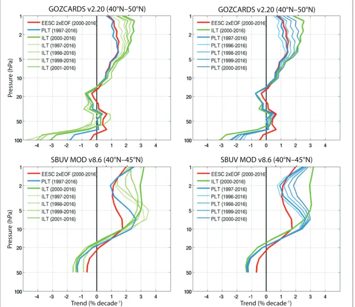
Both PLT and ILT trend estimates are sensitive to the start- and endpoints of the time series, but this sensitivity decreases as the length of the time series increases. For stratospheric ozone trends, the ad-vantages of ILT over PLT are that outliers in the mid 1990s affect only one trend, not both, and that no linear model is forced during the turnaround period, when the time series behaves nonlinearly. The inflec-tion time in the PLT model is generally fixed to ~1997 (Harris et al., 2008; Kyrölä et al., 2013; Chehade et al., 2014; Damadeo et al., 2014), coinciding with the turnaround in ODS concentrations (see Chapter 1). Changing this inflection point impacts PLT trends in the upper stratosphere; for datasets that end in 2016, PLT trends systematically increase by up to 0.3% decade−1 _{(at mid-latitudes) for every forward} shift in inflection time of one year. Changing the start year for recovery in the ILT analyses from 1997 to 2000 leads to a change in the trends of up to 1–1.5% decade−1 _{(Figure 3-8; LOTUS, 2018). Hence, trends} calculated over different time periods are not directly comparable, and the level of disagreement depends on the trend model and the dataset (LOTUS, 2018).

SAGE-CCI-OMPS v1 (35°–60°N, 42 km) Year Ozone anomaly (%) +2 -10 +10 -6 -2 0 +2 +6 -10 +10 -6 -2 0 +2 +6 -2 +2 0 0 -2 -2 +2 0 0 -2 -2 1979 1982 1985 1988 1991 1994 1997 2000 2003 2006 2009 2012 2015 2018 1979 1982 1985 1988 1991 1994 1997 2000 2003 2006 2009 2012 2015 2018 1979 1982 1985 1988 1991 1994 1997 2000 2003 2006 2009 2012 2015 2018 Satellite observations Solar cycle QBO ENSO Stratospheric aerosol

Regressed natural variations + ILT trends

Regressed ILT trends

Regressed natural variations

Residuals: Observations –(regressed natural variations + ILT trends)

Figure 3-7. Terms in the regression of monthly deseasonalized ozone anomalies from SAGE-CCI-OMPS at

42 km in the 35°–60°N zonal band. The top panel shows observed monthly mean anomalies (in %; gray line) relative to the annual cycle of ozone. The black line is the result of the regression model including the inde-pendent linear trends (ILTs; thick blue lines). The light blue line shows the sum of the terms of the regression model without the ILTs included. The middle panel shows the residual in the observed ozone when the long-term trend and regressed natural variations are subtracted. The bottom panel shows the relative contribu-tions of (from top to bottom) the solar flux, QBO, ENSO, and aerosols to the reconstructed time series (light blue line) in the top panel. The same vertical scale is used for all time series. Dashed lines fall outside the period used by the MLR. Observations and regression model are those used by LOTUS (2018).

This issue should not be overlooked when comparing trends and their significance from different analyses. Long-term changes in ozone can also be represented as a nonlinear process; e.g., proportional to a measure

of total stratospheric halogen loading such as an EESC proxy. EESC is calculated from emission rates of chlo-rofluorocarbons and related halogenated compounds, given their individual Ozone Depletion Potentials (ODPs) and certain assumptions regarding transport

Figure 3-8. Sensitivity of ozone profile trend estimates to the modeling of the trend in the regression

(independent, piecewise, or EESC) and its starting point. Results are shown for GOZCARDS v2.20 (top row) and SBUV MOD v8.6 (bottom row) at mid-northern latitudes for the past two decades. Trends in the upper stratosphere vary by 1–2 % decade−1 _{depending on the trend model and regression period. Adapted from}

LOTUS (2018). SBUV MOD v8.6 (40°N–45°N) GOZCARDS v2.20 (40°N–50°N) SBUV MOD v8.6 (40°N–45°N) GOZCARDS v2.20 (40°N–50°N) Pr essure (hP a) Pr essure (hP a)

Trend (% decade-1_{) Trend (% decade}-1₎

times into the stratosphere. EESC-derived trends are primarily used for attribution studies. They are not well suited to detection of recent trends because the model uses a single fit coefficient, which is primarily constrained by the early period of large EESC increas-es and ozone depletion ratincreas-es. The small ozone changincreas-es observed in recent years are poorly described by the modest post-turnaround decline in EESC (Damadeo et al., and 2014; Frith et al., 2017). In fact, the strong anti-correlation between EESC and ozone in the early period can force an erroneous, statistically significant

positive trend in the latter period, even through syn-thetic time series in which EESC does not decrease (Kuttippurath et al., 2015). Models with two orthog-onal EESC terms avoid such trend bias by effectively leaving the turnaround time and ozone depletion/re-covery rate as free parameters (Damadeo et al., 2014, 2018), but this renders attribution of trends to chang-es in ODSs lchang-ess straightforward. Adaptive techniquchang-es, such as dynamic linear regression models (DLMs; Laine et al., 2014, and Ball et al., 2017) and ensem-ble empirical mode decomposition (EEMD) methods