HAL Id: hal-01635617
https://hal.archives-ouvertes.fr/hal-01635617
Submitted on 15 Nov 2017
HAL is a multi-disciplinary open access
archive for the deposit and dissemination of
sci-entific research documents, whether they are
pub-lished or not. The documents may come from
teaching and research institutions in France or
abroad, or from public or private research centers.
L’archive ouverte pluridisciplinaire HAL, est
destinée au dépôt et à la diffusion de documents
scientifiques de niveau recherche, publiés ou non,
émanant des établissements d’enseignement et de
recherche français ou étrangers, des laboratoires
publics ou privés.
ENVIRONMENT MODELING FROM IMAGES
TAKEN BY A LOW COST CAMERA
Maxime Lhuillier
To cite this version:
Maxime Lhuillier. ENVIRONMENT MODELING FROM IMAGES TAKEN BY A LOW COST
CAMERA. The ISPRS Commission III symposium on Photogrammetric Computer Vision and Image
Analysis, Sep 2010, Paris, France. �hal-01635617�
ENVIRONMENT MODELING FROM IMAGES TAKEN BY A LOW COST CAMERA
Maxime Lhuillier
LASMEA, UMR 6602 Universit´e Blaise Pascal/CNRS, 63177 Aubi`ere Cedex, France, http://maxime.lhuillier.online.fr
Commission III/1
KEY WORDS: catadioptric camera, multi-view geometry estimation, environment reconstruction, vision system
ABSTRACT:
This paper describes a system to generate 3D model from image sequence taken in complex environment including variable ground surface, buildings and trajectory loops. Here we use a $1000 catadioptric camera and an approximate knowledge of its calibration. This contrasts to current systems which rely on more costly hardware such as the (calibrated) spherical vision camera Ladybug. All steps of the method are summarized. Experiments include a campus reconstruction from thousands of images.
1 INTRODUCTION
The automatic 3D modeling of environment from image sequence is a long-term and still active field of research. Wide view field camera is a natural choice for ground-based sequence. Current systems include multi-camera and accurate GPS and INS (Polle-feys et al., 2008) at high cost (>$100K), the Ladybug
multi-camera (www.ptgrey.com, 2010) at medium cost (≈$12K). Here
we use a catadioptric camera at low cost (≈$1K): a mirror of
revolution (www.0−360.com, 2010) mounted on a perspective
still camera (Nikon Coolpix 8700) thanks to adapter ring. The medium and high cost systems are more convenient since they provide video sequences and wide view field without sacrificing image resolution.
The first step is the estimation of successive camera poses using Structure-from-Motion (SfM). Recent work (Micusik and Kosecka, 2009) suggests that bundle adjustment (BA) is not needed if sev-eral good experimental conditions are meet: large resolution, wide view field, and accurate knowledge of calibration. Here we do not require accurate calibration since it depends on both mirror pro-file (mirror manufacturer may not like to reveal it) and the pose between the perspective camera and the mirror. Furthermore, we would like to avoid calibration pattern handling for end-users. For these reasons, BA is needed to estimate simultaneously cam-era poses, reconstructed points and intrinsic parameters.
Drift or error accumulation occurs in SfM of long image sequences. It should be detected between images taken at similar locations in the scene (Anan and Hartley, 2005, Havlena et al., 2009) and re-moved using BA (Cornelis et al., 2004). Here we remove drift us-ing constrained bundle adjustment (CBA) based on (Triggs et al., 2000), instead of a re-weighted version of the standard BA (Cor-nelis et al., 2004) which relies much on heuristic initialization. The next step is the estimation of the 3D scene. Like (Polle-feys et al., 2008, Micusik and Kosecka, 2009), we apply dense stereo method on a small number ofM consecutive images,
it-erate this process several times along the sequence, and merge the obtained view-centered 3D models into the global and final 3D model. Furthermore, we use an over-segmentation in the ref-erence image of view-centered model in conjunction with dense stereo (Zitnick and Kang, 2007, Micusik and Kosecka, 2009). Super-pixels (small regions) are useful to reduce stereo ambigu-ity, to constrain depth discontinuities at super-pixel borders se-lected among image contours, to reduce computational complex-ity.
Our over-segmentation is defined by triangle mesh in image such that (1) super-pixel is a list of connected triangles and (2) trian-gles of the view-centered model are back-projected triantrian-gles of the image mesh. In work (Zitnick and Kang, 2007, Micusik and Kosecka, 2009), super-pixel is pixel list and is unused by surface meshing. Our choice has several advantages. Mesh regularizes super-pixel shape and defines the resolution of final reconstruc-tion by view field sampling. This is useful to compress large scene. Besides, we obtain triangles in 3D such that the consis-tency with image contours can not be degraded by depth error unlike (Chai et al., 2004). This is not a luxury because depth esti-mation is difficult in uncontrolled environment. Our super-pixels are not restricted to be planar in 3D contrary to those in (Zitnick and Kang, 2007, Micusik and Kosecka, 2009).
The last step is filtering of triangles in view-centered models. It reduces the redundancy and removes the most inaccurate and un-expected triangles. Here we accept non-incremental method with complexity greater than linear in the number of camera poses, since the main calculations are done in the previous step (which has linear complexity and is parallelizable using multi-cores). This paper improves work (Lhuillier, 2008a, Lhuillier, 2008b) thanks to polygons for super-pixels, drift removal using CBA, ac-celerations for larger sequence (feature selection in the SfM step, complexity handling in the triangle filtering step), redundancy re-duction, experiments on more challenging sequence.
2 OVERVIEW OF THE RECONSTRUCTION METHOD
This Section has six parts describing camera model, Structure-from-Motion, drift removal, over-segmentation mesh, view-cen--tered model and triangle filtering.
2.1 Camera Model
A single view-point camera model with a general radial distortion function and a symmetry axis is used (Lhuillier, 2008a). It simpli-fies the reconstruction process for non-single view-point camera (if any), assuming that depth is large enough.
We assume that the projection of the whole view field is delim-ited by two concentric circles which can be detected in images. Furthermore, the mirror manufacturer provides the lower an d up-per bounds of the “ray angle” between observation ray and the symmetry axis. The initial calibration is that of equiangular cam-era: the mapping from the ray angle of 3D point to the distance between the point projection and the circle center is linear.
2.2 Structure-from-Motion
Structure-from-Motion (Lhuillier, 2008a) is applied to estimate geometry (camera poses and a sparse cloud of 3D points) using the calibration initialization of Section 2.1: estimate the 2-view and 3-view geometries of consecutive images from matched Har-ris points (step 1) and then estimate the whole sequence geometry using bundle adjustment (BA) applied in a hierarchical frame-work (step 2). Another BA is applied to refine simultaneously radial distortion parameters and the 3D assuming that the radial distortion is constant in the whole sequence (step 3).
Although it is important to get a maximum number of recon-structed features for 3D scene modeling, we noticed that there are many more 3D points than needed to initialize the geometry in our wide view field context. Indeed, this is not uncommon to have more than 2000 features per outdoor image involved in BA, and this implies a waste of computation time. So the numbernf
of features per image is limited to 500 in all BAs of steps 1-2-3: 3D points are randomly selected and removed whilenf is larger
than 500 in all images. In practice, this simple scheme holds a good point distribution in the view field. The4th
step is the fol-lowing: step 3 is applied a second time withoutnf limit to get
a maximum number of reconstructed features consistent with the poses and calibration.
Our BA is the sparse Levenberg-Marquardt method assuming that there are more structure parameters than camera ones: it includes profile Choleski decomposition (Triggs et al., 2000) of the re-duced camera system.
2.3 Drift Removal
Drift or error accumulation is unavoidable in the geometry esti-mation of long sequence. Methods (Havlena et al., 2009, Anan and Hartley, 2005, Cornelis et al., 2004) detect the drift between two reconstructed imagesi and j if these images are taken at
similar locations. These methods also provide listLi,jof point
matches betweeni and j, which is used to remove drift. Without
drift removal, scene part visible ini and j is reconstructed twice.
Adequate BA and its initialization are applied to remove recon-struction duplicates while maintaining low re-projection errors in the whole sequence of images{0, 1 · · · n − 1}. Once the 2D
fea-ture match listLi,j is given for pair{i, j}, we remove the drift
betweeni and j as follows. First, we choose integer k such that
the neighborhoodN (i) of i is the list {i − k · · · i · · · i + k}.
Sec-ond,N (i) and its data (3D geometry and image features) are
du-plicated in imagesN (n + k) = {n · · · n + 2k} such that images n + k and i are the same. Third, we use RANSAC to fit the
simi-larity transformations of 3D points matched by Li,jand applys
to obtainN (n + k) geometry in the same basis as {0 · · · n − 1}
geometry. Fourth,{0 · · · n + 2k} geometry is refined by BA
tak-ing into accountLn+k,j (Ln+k,jis a copy of Li,j with image
index changes). NowN (n + k) geometry is the drift correction
ofN (i) geometry. Fifth, constrained bundle adjustment (CBA)
is applied to minimize the global re-projection error subject to constraintc(x) = 0, where x concatenates 3D parameters of {0 · · · n + 2k} and c(x) concatenates the drifts between poses
ofN (i) and N (n + k) (more details in Appendix B). At this
point, the drift betweeni and j is removed but N (n + k) is
re-dundant. Last, we remove data involvingN (n + k) and apply
BA to{0 · · · n − 1} geometry by taking into account Li,j.
This scheme is applied using a limit ofnf = 500 features per
image to avoid waste of time as in Section 2.2, with the only difference thatLi,jandLn+k,jare not counted by this limit.
2.4 Over-Segmentation Mesh
This mesh has the following purposes. It makes image-based sim-plification of the scene such that the view field is uniformly sam-pled. This is useful for time and space complexities of further processing and more adequate than storing depth maps for all im-ages. Furthermore, it segments the image into polygons such that depth discontinuities are constrained to be at polygon borders. These borders are selected among image contours. If contours are lacking, borders are preferred on concentric circles or radial segments of the donut image. This roughly corresponds to hori-zontal and vertical depth discontinuities for standard orientation of the catadioptric camera (if its symmetry axis is vertical). In short, the image mesh is build in four steps: initialization checkerboard (rows are concentric rings, columns have radial di-rections, cells are two Delaunay triangles), gradient edge inte-gration (perturb vertices to approximate the most prominent im-age contours), optimization (perturb all vertices to minimize the sum, for all triangles, of color variances, plus the sum, for all ver-tices, of squared moduluses of umbrella operators), and polygon segmentation (triangles are regrouped in small and convex poly-gons). In practice, lots of polygons are quadrilaterals similar to those of the initialization checkerboard.
2.5 View-Centered 3D Model
View-centered 3D model is build from image mesh (Section 2.4) assuming that the geometry is known (Sections 2.1, 2.2 and 2.3).
Depth Map in the Reference Image We reproject catadioptric image onto the 6 faces of a virtual cube and apply match prop-agation (Lhuillier and Quan, 2002) to two parallel faces of two cubes. The depth map in theith
image is obtained by chaining matches between consecutive images ofN (i). In the next steps,
the over-segmentation mesh in theithimage is back-projected to
approximate the depth map.
Mesh Initialization For all polygons in imagei, a plane in 3D
(or nil if failure) is estimated by a RANSAC procedure applied on depths available inside the polygon. A depth is inlier of ten-tative plane if the corresponding 3D point is in this plane up to thresholding (Appendix A). The best planeπ defines 3D points
which are the intersections betweenπ and the observation rays of
the polygon vertices in theithimage. These 3D points are called
“3D vertices of polygon” although the polygon is 2D.
For all edgese in image i, we define boolean bewhich will
deter-mine the connection of triangles in both edge sides. Since depth discontinuity is prohibited inside polygons, we initializebe = 1
if both triangles are in the same polygon (other cases:be= 0).
Connection Connections between polygons are needed to ob-tain a more realistic 3D model. Thus edge booleans are forced to
1 if neighboring polygons satisfy coplanarity constraint. For all
polygonsp with a plane in 3D, we collect in list Lpthe polygons
q in p-neighborhood (including p) such that all 3D vertices of q
are in the plane ofp up to thresholding (Appendix A). If the sum
of solid angles of polygons inLpis greater than a threshold, we
have confidence in coplanarity between all polygons inLpand
we setbe= 1 for all edges e between two polygons of Lp.
Hole Filling We fill holeH if its neighborhood N is
copla-nar. BothH and N are polygon lists. The former is a connected
component of polygons without plane in 3D and the latter con-tains polygons with plane in 3D. NeighborhoodN is coplanar if
there is a planeπ (generated by random samples of vertices of N ) such that all 3D vertices in N are in π up to thresholding
(Appendix A). IfN is coplanar, all polygons of H get plane π
View-Centered Mesh in 3D Now, 3D triangles are generated by back-projection of triangles in the image mesh using polygon planes and edge booleans. Trianglet inside a polygon p with
plane in 3D is reconstructed as follows. LetCvbe the
circularly-linked list of polygons which have vertexv of t. We obtain
sub-list(s) ofCvby removing theCv-links between consecutive
poly-gons which share edgese such that be = 0. A Cv-link is also
removed if one of its two polygons has not plane in 3D. LetSp v
be the sub-list which containsp. The 3D triangle of t is defined
by its 3 vertices: the 3D vertex reconstructed forv is the mean of
3D vertices of the polygons inSp
vwhich correspond tov.
Refinement Here we provide a brief overview of the refine-ment, which is detailed in (Lhuillier, 2008b). The view-centered mesh (3D triangles with edge connections) is parametrized by the depths of its vertices and is optimized by minimizing a weighted sum of discrepancy and smoothing terms. The discrepancy term is the sum, for all pixels in a triangle with plane in 3D, of the squared distance between the plane and 3D point defined by pixel depth (Appendix A). The smoothing term is the sum, for all edges which are not at image contour, of the squared difference between normals of 3D triangles in both edge sides. This minimization is applied several times by alternating with mesh operations “Trian-gle Connection” and “Hole Filling” (Lhuillier, 2008b).
2.6 Triangle Filtering
For alli, the method in Section 2.5 provides a 3D model centered
at imagei using images N (i). Now, several filters are applied on
the resulting list of triangles to remove the most inaccurate and unexpected triangles.
Notations We need additional notations in this Section. Here
t is a 3D (not 2D) triangle of the ithview-centered model. The
angle between two vectors u and v is angle(u, v) ∈ [0, π]. Let di, ci be the camera symmetry direction and center at theith
pose in world coordinates (dipoints toward the sky). LetUj(v)
be the length of major axis of covariance matrix Cvof v ∈ R 3
as if v is reconstructed by ray intersection from v projections in imagesN (j) using Levenberg-Marquardt.
Uncertainty Parts of the scene are reconstructed in several view-centered models with different accuracies. This is especially true in our wide view field context where a large part of the scene is visible in a single image. Thus, the final 3D model can not be de-fined by a simple union of the triangle lists of all view-centered models. A selection on the triangles should be done.
We rejectt if the ith
model does not provide one of the best avail-able uncertainties from all models: if all vertices v oft have ratio Ui(v)/ minjUj(v) greater than threshold u0.
Prior Knowledge Here we assume that the catadioptric cam-era is hand-held by a pedestrian walking on the ground such that (1) the camera symmetry axis is (roughly) vertical (2) the ground slope is moderated (3) the step length between consecutive im-ages and the height between ground and camera center do not change too much. This knowledge is used to reject unexpected triangles which are not in a “neighborhood of the ground”. A step length estimate iss = mediani||ci− ci+1||. We choose
anglesαt, αb between di and observation rays such that0 <
αt < π2 < αb < π. Triangle t is rejected if it is below the
ground: if it has vertex v such that angle(di, v − ci) > αband
height 1sdTi(v − ci) is less than a threshold. The sky rejection
does not depend on scales. We robustly estimate the mean m
and standard deviationσ of height dT
i(v − ci) for all vertex v
of theith
model such that angle(di, v − ci) < αt. Trianglet is
rejected if it has vertex v such that angle(di, v − ci) < αtand 1
σ(d T
i(v − ci) − m) is greater than a threshold.
Reliability 3D modeling application requires additional filter-ing to reject “unreliable” triangles that filters above miss. These triangles includes those which are in the neighborhood of the line supporting the cj, j ∈ N (i) (if any). Inspired by a two-view
reliability method (Doubek and Svoboda, 2002), we rejectt if it
has vertex v such thatmaxj,k∈N (i)angle(v − cj, v − ck) is less
than thresholdα0. This method is intuitive: t is rejected if ray
directions v− cj, j ∈ N (i) are parallel.
Redundancy Previous filters provide a redundant 3D model in-sofar as scene parts may be reconstructed by several mesh parts selected in several view-centered models. Redundancy increases with thresholdu0 of the uncertainty-based filter and the inverse
of thresholdα0of the reliability-based filter. Our final filter
de-creases redundancy as follows: 3D triangles at mesh borders are progressively rejected in the decreasing uncertainty order if they are redundant with other mesh parts. Trianglet is redundant if its
neighborhood intersects triangle of thejth
view-centered model (j 6= i). The neighborhood of t is the truncated pyramid with
baset and three edges. These edges are the main axes of the 90%
uncertainty ellipsoids of thet vertices v defined by Cv.
Complexity Handling We apply the filters above in the in-creasing complexity order to deal with large number of trian-gles (tens of millions in our case). Filters based on prior knowl-edge and reliability are applied first. Thanks to cj and
relia-bility angleα0, we estimate radius ri and center bi of a ball
which encloses the selected part of theith
view-centered model:
bi= 12(ci−1+ ci+1) and tan(α0/2) = ||ci+1− ci−1||/(2ri) if
N (i) = {i − 1, i, i + 1}. Let N(i) = {j, ||bi− bj|| ≤ ri+ rj}
be the list of view-centered modelsj which may have
intersec-tion with the ith view-centered model. Then the
uncertainty-based filter is accelerated thanks toN (i): triangle t is rejected
ifUi(v)/ minj∈N(i)Uj(v) ≥ u0 for all vertices v oft. Last,
the redundancy-based filter is applied. Its complexity due to un-certainty sort isO(p log(p)), where p is the number of triangles.
Its complexity due to redundancy triangle tests isO(p2), but this
is accelerated using test eliminations and hierarchical bounding boxes.
3 EXPERIMENTS
The image sequence is taken in the university campus on au-gust 15-16th afternoons without people. There are several tra-jectory loops, variable ground surface (road, foot path, unmown grass), buildings, corridor and vegetation (bushes, trees). This scene accumulates several difficulties: not 100% rigid scene (due to breath of wind), illuminations changes between day 1-2 sub-sequences (Fig 2), low-textured areas, camera gain changes (un-corrected), aperture problem and non-uniform sky at building-sky edges. The sequence has 22603264 × 2448 JPEG images, which
are reduced by 2 in both dimensions to accelerate all calculations. The perspective camera points toward the sky, it is hand-held and mounted on a monopod. The mirror (www.0−360.com, 2010)
provides large view field: 360 degrees in the horizontal plane, about 52 degrees above and 62 degrees below. The view field is projected between concentric circles of radii 572 and 103 pixels. We use a core 2 duo 2.5Ghz laptop with 4Go 667MHz DDR2. First, the geometry is estimated thanks to the methods in Sec-tions 2.1, 2.2 and 2.3. The user provides the list of image pairs
{i, j} such that drift between i and j should be removed (drift
de-tection method is not integrated in the current version of the sys-tem). Once the geometry of days 1 and 2 sub-sequences are es-timated using the initial calibration, points are matched between imagesi and j using correlation (Fig. 2) and CBA is applied to
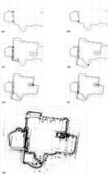
Figure 1: Geometry estimation steps: (a) day 1 sequence, (b) re-move drift, (c) merge day 1-2 sequences, (d-f) rere-move drifts, (g) use all features. All results are registered in rectangle [0, 1] × [0, 0.8] by enforcing constant coordinates on the two poses
sur-rounded by gray disks in (a). Gray disks in (b,d,e,f) show poses where drift is corrected. Day 1-2 sequences are merged on gray disk in (c).
remove drifts usingk = 1. Cases (b,d,e,f) of Fig. 1 are
trajec-tory loops with (424,451,1434,216) images and are obtained by (16,62,39,9) CBA iterations in (190,2400,1460,370) seconds, re-spectively. We think that a large part of the drift in case (d) is due to the single view point approximation, which is inaccurate in the outdoor corridor (top right corner of Fig. 4) with small scene depth. A last BA is applied to refine the geometry (3D and intrinsic parameters) and to increase the list of reconstructed points. The final geometry (Fig. 1.g) has 699410 points recon-structed from 3.9M Harris features; the means of track lengths and 3D points visible in one view are 5.5 and 1721, respectively. Then, 2256 view-centered models are reconstructed thanks to the methods in Section 2.4 and 2.5 usingk = 1. This is the most time
consuming part of the method since one view-centered model is computed in about 3 min 30s. The first step of view-centered model computation is the over-segmentation mesh in the refer-ence image. It samples the view field such that the super-pixels at the neighborhood of horizontal plane projection are initialized by squares of size8 × 8 pixels in the images. The mean of number
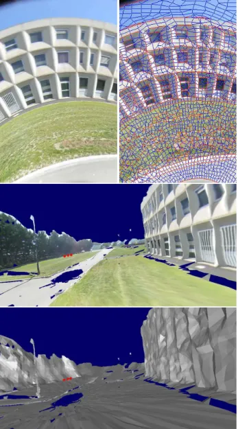
of 3D triangles is 17547. Fig. 3 shows super-pixels of a reference image and the resulting view-centered model.
Figure 2: From top to bottom: 722 and 535 matches ofLi,jused
to remove drift in cases (d) and (e) of Fig. 1. Images of days 1 and 2 are on the left and right, respectively.
Last, the methods in Section 2.6 are applied to filter the 39.6M triangles stored in hard disk. A first filtering is done using relia-bility (α0 = 5 degrees), prior knowledge and uncertainty filters
(u0= 1.1): we obtain 6.5M triangles in 40 min and store them in
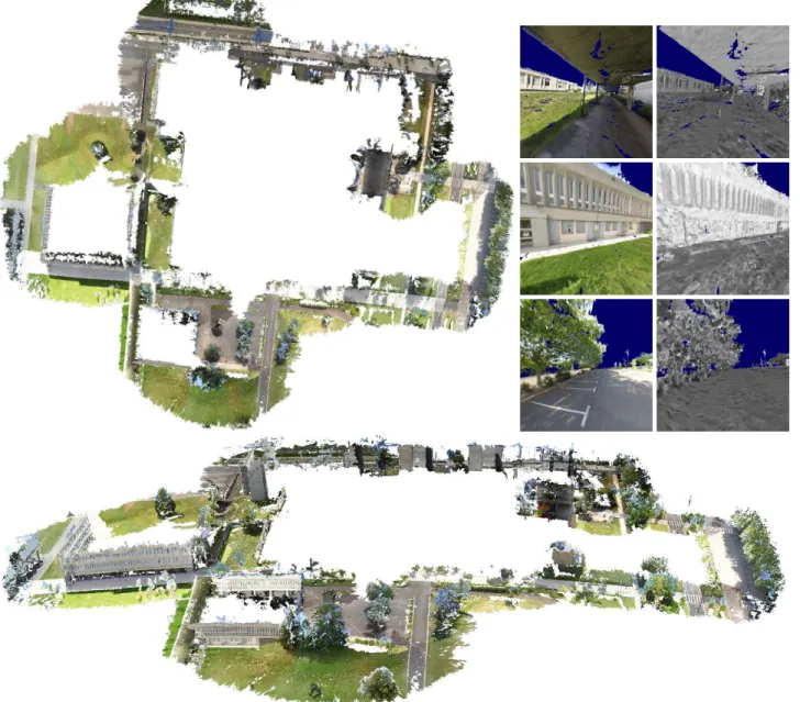
RAM. Redundancy removal is the last filtering and selects 4.5M triangles in 44 min. Texture packing and VRML file saving take 9 min. Fig. 4 shows views of the final model. We note that the scene is curved as if it lie on a sphere surface whose diameter has several kilometers: a vertical component of drift is left.
An other experiment is the quantitative evaluation of scene ac-curacy (discrepancy between scene reconstruction and ground truth) for a view-centered model using k = 1. A
represen-tative range of baselines is obtained with the following ground truth: the [0, 5]3 cube and camera locations defined by c
i =
`1 1 + i/5 1´T
, i ∈ {0, 1, 2} (numbers in meters). First,
synthetic images are generated using ray-tracing and the knowl-edge of mirror/perspective camera/textured cube. Second, meth-ods in Sections 2.1, 2.2, 2.4 and 2.5 are applied. Third, a camera-based registration is applied to put the scene estimation in the coordinate frame of ground truth. Last, the scene accuracya0.9
is estimated using the distancee between vertex v of the model
and the ground truth surface: inequality|e(v)| ≤ a0.9||v − c1||
is true for 90% of vertices. We obtaina0.9= 0.015.
4 CONCLUSION
We present an environment reconstruction system from images acquired by a $1000 camera. Several items are described: camera model, structure-from-motion, drift removal, view field sampling by super-pixels, view-centered model and triangle filtering. Un-like previous work, image meshes define both super-pixels (con-vex polygons) and triangles of 3D models. The current system is fully automatic up to the loop detection step (that previous methods could solve). Last it is experimented on a challenging sequence.
Future work includes loop detection integration, better use of visibility and prior knowledge for scene reconstruction, joining
Figure 4: Top view (top left), local views (top right) and oblique view (bottom) of the final 3D model of the campus. The top view can be matched with Fig. 1.g. The transformation between top and oblique views is a rotation around horizontal axis.
meshes of view-centered models to form a continuous surface, and accelerations using GPU.
REFERENCES
Anan, C. S. and Hartley, R., 2005. Visual localization and loop-back detection with a high resolution omnidirectional camera. In: OMNIVIS Workshop.
Chai, B., Sethuraman, S., Sawhney, H. and Hatrack, P., 2004. Depth map compression for real-time view-based rendering. Pat-tern recognition letters 25(7), pp. 755–766.
Cornelis, K., Verbiest, F. and Gool, L. V., 2004. Drift removal for sequential structure from motion algorithms. PAMI 26(10), pp. 1249–1259.
Doubek, P. and Svoboda, T., 2002. Reliable 3d reconstruction from a few catadioptric images. In: OMNIVIS Workshop. Havlena, M., Torri, A., Knopp, J. and Pajdla, T., 2009. Ran-domized structure from motion based on atomic 3d models from camera triplets. In: CVPR’09.
Lhuillier, M., 2008a. Automatic scene structure and camera mo-tion using a catadioptric system. CVIU 109(2), pp. 186–203. Lhuillier, M., 2008b. Toward automatic 3d modeling of scenes using a generic camera model. In: CVPR’08.
Lhuillier, M. and Quan, L., 2002. Match propagation for image-based modeling and rendering. PAMI 24(8), pp. 1140–1146. Micusik, B. and Kosecka, J., 2009. Piecewise planar city 3d mod-eling from street view panoramic sequence. In: CVPR’09. Pollefeys, M., Nister, D., Frahm, J., Akbarzadeh, A., Mordohai, P., Clipp, B., Engels, C., Gallup, D., Kim, S., Merell, P., Salmi, C., Sinha, S., Talton, B., Wang, L., Yang, Q., Stewenius, H., Yang, R., Welch, G. and Towles, H., 2008. Detailed real-time urban 3d reconstruction from video. IJCV 78(2), pp. 143–167. Schindler, K. and Bischof, H., 2003. On robust regression in photogrammetric point clouds. In: DAGM’03.
Triggs, B., McLauchlan, P., Hartley, R. and Fitzgibbon, A., 2000. Bundle adjustment – a modern synthesis. In: Vision Algorithms Workshop.
Figure 3: From top to bottom: part of reference image, over-segmentation using polygons (contours in red), view-centered model (texture and normals) reconstructed from 3 poses (in red). www.0−360.com, 2010.
www.ptgrey.com, 2010.
Zitnick, C. and Kang, S., 2007. Stereo for image-based rendering using image over-segmentation. IJCV 75(1), pp. 49–65.
APPENDIX A: POINT AND PLANE THRESHOLDING
Let p be a 3D point. The covariance matrix Cp of p is
pro-vided by ray intersection from p projections in imagesN (i) = {i − k · · · i · · · i + k} using Levenberg-Marquardt. In this
pa-per, ray intersection and covariance Cpresult from the angle
er-ror in (Lhuillier, 2008b). The Mahalanobis distanceDpbetween
points p and p′isDp(p
′) =q(p − p′)TC−1
p (p − p′).
We define points p= ci+ zu and p′= ci+ z′u using camera
location ci, ray direction u and depthsz, z′. Ifz is large enough,
u is a good approximation of the main axis of Cp: we have Cp≈
σ2 puu T and uTC−1 p u ≈ σ −2 p whereσ 2
p is the largest singular
value of Cp. In this context, we obtainDp(p
′) ≈|z−z′|
σp .
If x has the Gaussian distribution with mean p and covariance
Cp,Dp2(x) has the X
2distribution with 3 d.o.f. We decide that
points p and p′ are the same (up to error) if bothDp2(p ′) and
D2
p′(p) are less than the 90% quantile of this distribution: we
decide that p and p′are the same point ifD(p, p′) ≤ 2.5 where D(p, p′) = max{Dp(p ′), D p′(p)} ≈ |z−z′| min{σp,σp′} .
Letπ be the plane nTx+d = 0. The point-to-plane Mahalanobis
distance isD2 p(π) = minx∈πD 2 p(x) = (nTp+d)2 nTCpn (Schindler
and Bischof, 2003). Thus Cp ≈ σ 2 puu T and p′ ∈ π imply D2 p(π) ≈ (nT p′+d+nT(p−p′))2 σ2p(nTu)2 = (z−z′)2 σ2 p ≈ D2 p(p ′).
Last, we obtain the point-to-plane thresholding and distance used in Section 2.5. We decide that p is in planeπ if D(p, p′) ≤ 2.5 where p′ ∈ π. The robust distance between p and π is min{D(p, p′), 2.5} ≈ min{min{σ|z−z′|
p,σp′}
, 2.5}, z′= −nTci+d
nTu .
APPENDIX B: CONSTRAINED BUNDLE ADJUSTMENT
In Section 2.3, we would like to apply CBA (constrained bun-dle adjustment) summarized in (Triggs et al., 2000) to remove the drift. This method minimizes the re-projection error func-tion x7→ f (x) subject to the drift removal constraint c(x) = 0,
where x concatenates poses and 3D points. Here we havec(x) = x1 − xg1 where x1 and xg1 concatenate 3D locations of images
N (i) and their duplicates of images N (n + k), respectively. All
3D parameters of sequence{0 · · · n + 2k} are in x except the 3D
locations ofN (j) and N (n + k). During CBA, xg
1is fixed and
x1evolves towards xg1.
However, there is a difficulty with this scheme. CBA iteration (Triggs et al., 2000) improves x by adding step ∆ which mini-mizes quadratic Taylor expansion off subject to 0 ≈ c(x + ∆)
and linear Taylor expansionc(x + ∆) ≈ c(x) + C∆. We use
no-tations xT =`xT
1 xT2´, ∆T =`∆1T ∆T2´, C = `C1 C2´
and obtain C1 = I, C2 = 0. Thus, we have ∆1= −c(x) at the
first CBA iteration. On the one hand, ∆1 = −c(x) is the drift
and may be very large. On the other hand, ∆ should be small enough for quadratic Taylor approximation off .
The “reduced problem” in (Triggs et al., 2000) is used: BA itera-tion minimizes the quadratic Taylor expansion of ∆27→ g(∆2)
whereg(∆2) = f (∆(∆2)) and ∆(∆2)T =`−c(x)T ∆T2´.
Step ∆2 meets H2(λ)∆2 = −g2, where(λ, g2, H2(λ)) are
damping parameter, gradient and damped hessian ofg. Update x← x + ∆(∆2) holds if g(∆2) < min{1.1f0, g(0)}, where
f0 is the value off (x) before CBA. It can be shown that this
inequality is true ifc(x) is small enough and λ is large enough.
Here we resetc by cnat thenthiteration of CBA to have a small
enoughc(x). Let x0
1 be the value of x1 before CBA. We use
cn(x) = x1− ((1 − γn)x10+ γnxg1), where γnincreases
pro-gressively from0 (no constraint at CBA start) to 1 (full constraint
at CBA end). One CBA iteration is summarized as follows. First, estimate ∆2(γn) for the current value of (λ, x) (a single linear
systemH2(λ)X = Y is solved for all γn ∈ [0, 1]). Second, try
to increaseγnsuch thatg(∆2(γn)) < min{1.1f0, g(0)}. If the
iteration succeeds, apply x← x + ∆(∆2). Furthermore, apply
λ ← λ/10 if γn= γn−1. If the iteration fails, applyλ ← 100λ.
Ifγn > γn−1orγn = 1, choose γn+1 = γnat the(n + 1)th
iteration to obtain∆(∆2)T =`0T ∆T2´ and to decrease f as