D-efficient or deficient? A robustness analysis
of stated choice experimental designs
The MIT Faculty has made this article openly available.
Please share
how this access benefits you. Your story matters.
Citation
Walker, Joan L., et al. “D-Efficient or Deficient? A Robustness
Analysis of Stated Choice Experimental Designs.” Theory and
Decision, vol. 84, no. 2, Mar. 2018, pp. 215–38.
As Published
http://dx.doi.org/10.1007/s11238-017-9647-3
Publisher
Springer US
Version
Author's final manuscript
Citable link
http://hdl.handle.net/1721.1/114301
Terms of Use
Creative Commons Attribution-Noncommercial-Share Alike
1
D-EFFICIENT OR DEFICIENT?
A Robustness Analysis of Stated Choice Experimental Designs
Joan L Walker (corresponding author)
Department of Civil and Environmental Engineering & Center for Global Metropolitan Studies University of California, Berkeley
111 McLaughlin Hall, Berkeley CA 94720 [email protected]
Yanqiao Wang
Department of Civil and Environmental Engineering University of California, Berkeley
116 McLaughlin Hall, Berkeley CA 94720 [email protected]
Mikkel Thorhauge
Department of Management Engineering Technical University of Denmark
Bygningstorvet 116B, 2800 Kgs. Lyngby, Denmark [email protected]
Moshe Ben-Akiva
Department of Civil and Environmental Engineering Massachusetts Institute of Technology
Room 1-181, 77 Massachusetts Avenue, Cambridge, MA 02139 [email protected]
Submitted: November 2016
2
ABSTRACT
This paper is motivated by the increasing popularity of efficient designs for stated choice experiments. The objective in efficient designs is to create a stated choice experiment that minimizes the standard errors of the estimated parameters. In order to do so, such designs require specifying prior values for the parameters to be estimated. While there is significant literature demonstrating the efficiency improvements (and cost savings) of employing efficient designs, the bulk of the literature tests conditions where the priors used to generate the efficient design are assumed to be accurate. However, there is substantially less literature that compares how different design types perform under varying degree of error of the prior. The literature that does exist assumes small fractions are used (e.g., under 20 unique choice tasks generated), which is in contrast to computer aided surveys that readily allow for large fractions. Further, the results in the literature are abstract in that there is not a reference point (i.e., meaningful units) to provide clear insight on the magnitude of any issue. Our objective is to analyze the robustness of different designs within a typical stated choice experiment context of a trade-off between price and quality. We use as an example transportation mode choice, where the key parameter to estimate is the value of time (VOT). Within this context, we test many designs to examine how robust efficient designs are against a misspecification of the prior parameters. The simple mode choice setting allows for insightful visualizations of the designs themselves and also an interpretable reference point (VOT) for the range in which each design is robust. Not surprisingly, the D-efficient design is most efficient in the region where the true population VOT is near the prior used to generate the design: the prior is $20/hour and the efficient range is $10/hour -$30/hour. However, the D-efficient design quickly becomes the most inefficient outside of this range (under $5/hour and above $40/hour), and the estimation significantly degrades above $50/hour. The orthogonal and random designs are robust for a much larger range of VOT. The robustness of Bayesian efficient designs varies depending on the variance that the prior assumes. Implementing two-stage designs that first use a small sample to estimate priors are also not robust relative to uninformative designs. Arguably, the random design (which is the easiest to generate) performs as well as any design, and it (as well as any design) will perform even better if data cleaning is done to remove choice tasks where one alternative dominates the other. Keywords: stated choice experiments, robustness, mode choice model, value-of-time, experimental design, d-efficient.
3
1 INTRODUCTION
Within discrete choice models, data sources can be defined in one of two categories: Revealed Preference (RP) data and Stated Preference (SP) data. RP data is “observed” and relies on actual behavior. A number of disadvantages in using RP data, including little variation in the data and impracticality when dealing with new alternatives which are not yet available, have made the use of SP data a more popular method to estimate discrete choice models (Louviere and Hensher, 1982; Louviere and Woodworth, 1983). SP data are hypothetically created choice situations in which the researcher has the freedom to define the tradeoff faced by the respondent. SP data gained attention in the early 1970s after Davidson (1973) and Louviere et al. (1973) highlighted the desirable properties of SP studies, such as the evaluation of non-existing alternatives (Hensher, 1982; Louviere and Hensher, 1983) and the evaluation of choice with attributes that differ from the alternatives which currently exist (Kocur et al., 1982; Hensher and Louviere, 1983; Louviere and Kocur, 1983; Bradley and Bowy, 1984). However, the hypothetical nature of SP data is also its biggest criticism since SP data does not capture actual behavior (Cummings et al., 1986; Mitchell and Carson, 1989). For an in-depth discussion of advantages and disadvantages of RP and SP data see, for example, Adamowicz et al. (1994) and Hensher (1994).
We focus on stated choice (SC) experiments where the respondent is presented with hypothetical alternatives and asked to choose one. To create a stated choice design, one defines the alternatives that make up a choice set, determines the set of attributes that describe each alternative and, for each attribute, determine a set of discrete levels (i.e., values that the attribute can be). Then a set of specific choice contexts (i.e., specific alternatives with specific values of each attribute) that will be presented to respondents need to be defined. In the simple binary mode choice context used throughout this paper, an example choice context from which a respondent may be asked to make a choice is: alternative 1 costs $10 and takes 30 minutes and alternative 2 costs $4 and takes 60 minutes. Determining the sets of values (e.g., {($10, 30 minutes), ($4, 60 minutes)}) to use in the experiment is the art of experimental design. The full factorial design consists of all possible ways these attribute levels can be combined to make different choice sets. Typically, the full factorial design is extremely large and impractical to use in practice. Therefore, a subsample of the full factorial design, called a fractional factorial design, is selected for use in the experiment.
There are different ways to reduce the full factorial to the fraction that is used. One straightforward approach is to randomly select choice tasks from the full factorial design. However, the art of experimental design is to develop techniques that make this selection more thoughtfully so as to improve estimation results. The objective is typically to improve asymptotic efficiency (reduce standard errors of the estimates) while of course maintaining consistency of estimates (asymptotic unbiasedness). Orthogonal designs are a common approach for building SC designs. The motivation behind orthogonal designs is the ability to identify (i.e., estimate) the most important parameters in the model (i.e. the main effects) and also to estimate these parameters with precision (i.e., with minimal standard errors). A design is orthogonal if all the attributes in the design are uncorrelated, and it is also desirable to evenly distribute (i.e., balance) levels among the choice tasks (ChoiceMetrics, 2012). Although orthogonal designs are widely used and are optimal for linear regression (in terms of producing unbiased estimates with minimum standard error), they are not necessarily efficient for discrete choice analysis (Kuhfeld et al., 1994).
In recent years, efficient designs have emerged. The aim of efficient design is to minimize the standard error of the estimated model parameters. This is done via optimization based on the asymptotic variance-covariance (AVC) matrix. Unlike linear regression, the AVC matrix for discrete choice models is a function of the model parameters. Therefore, in order to minimize the AVC matrix for discrete choice, the values of the parameters must be known. However, the purpose of the model specification is to estimate the parameters, which are not known. To overcome this problem, efficient designs make use of prior parameter information as a best guess of the true parameters. Four different common strategies exist when defining the prior parameters. The first approach is to set the prior parameters equal to zero (a naïve prior). The second approach is to set the prior parameters to fixed, non-zero values. The third approach (introduced by Sándor and Wedel, 2001, 2002) is to define the prior parameters as coming from a known distribution with known parameters (Bliemer et al., 2008). A fourth approach is to update the design during the data collection phase as knowledge of the true parameters increases (Kanninen, 2002; Johnson et al., 2007 and 2013). Priors are sometimes determined based on pilot studies (Bliemer and Collins, 2016), but due to various reasons (such as time and budget constraints) researchers tends to rely solely on previous studies or expert judgement. Less known methods to generate the stated choice experiment exist, such as optimal orthogonal choice designs (see, e.g., Street et al., 2001, 2004, and 2005; Burgess and Street, 2005), and optimal choice probability
4
designs (Kanninen, 2002; Toner et al., 1999; Fowkes, 2000). Further, new approaches are regularly being presented, such as Bliemer and Collins’ (2016) proposal of a methodology to obtain priors without the need for conducting pilot studies. However, we keep our focus in this study on the most commonly used design approaches.
Studies in the literature have discussed the benefits and disadvantages of various methods and also compared subsets of methods. For example, Rose and Bliemer (2008) compared three different designs: optimal orthogonal design, efficient design, and optimal choice probability designs (where the latter two assume Bayesian prior parameters). Based on two different sets of prior parameters (one assumed to be correct and the second to test for misspecification), the authors highlight that different designs perform better under certain circumstances (and prior assumptions) and conclude that care is needed when constructing stated choice experiments since the choice of prior parameters can influence the design. Rose et al. (2008) studied a pivot design around a reference alternative and compared four different efficient designs with a traditional orthogonal design. They found that all four efficient designs outperformed the orthogonal design. Bliemer et al. (2008) compared several methods to generate Bayesian efficient designs and found that the quasi Monte Carlo methods (Halton, Sobol, and Modified Latin Hypercube Sampling) outperformed pseudo Monte Carlo draws, while the Gaussian quadrature method performed best. Rose and Bliemer (2009) compared a wide range of designs, such as orthogonal, efficient, optimal orthogonal, and optimal choice probability designs. They selected the level values and prior parameters arbitrarily and concluded that the optimal orthogonal design is better if all priors are assumed to be zero. The efficient design and optimal choice probability designs (which both rely on prior parameters) are superior when non-zero parameters are assumed, except at the outer most extreme areas of the interval range. Bliemer et al. (2009) extended the work on efficient designs for the Nested Logit (NL) model. They compared an efficient design (assuming correct priors) with two orthogonal designs (the orthogonal designs with the highest and lowest efficiency), and found that the D-error of the orthogonal designs was 2.1 and 7.4 times higher than the efficient design, respectively. They then proceeded to test for misspecification of 1) the priors, 2) the model type, and 3) nesting structures in the NL model. They found that the efficient design for the NL model is sensitive to a misspecification and that this effect can be mitigated by using a Bayesian efficient design. Furthermore, assuming a Multinomial Logit (MNL) form in the design phase leads to loss in efficiency, and thereby larger standard errors, if the true model form is a NL (though the loss in efficiency from NL to MNL is less critical). Finally, they found that specifying the nests incorrectly also leads to loss in efficiency. Bliemer and Rose (2010a) investigated a serial efficient design (or serial design), i.e. an efficient design in which the prior parameters are repeatedly updated as data is collected. They compared the serial design with an orthogonal and an efficient design. Results indicated that the serial design performed as well as an efficient design based on true parameters, and both outperformed the orthogonal design. The advantage of the serial design is that it is not sensitive to a misspecification of the priors, as these are constantly updated in accordance with collected data. The downside is that data collection is rather cumbersome. Bliemer and Rose (2010b) generated efficient designs for the Mixed Logit (ML) model and tested the performance in three case studies. They compared three efficient designs (using true parameters as priors) assuming the following model forms in the design phase: MNL model, cross-section ML model, and panel ML model. (In case study two they also compared a D-optimal orthogonal design assuming zero priors). Overall, they found that misspecification of the model form, e.g. constructing an experimental design assuming an MNL model form but relying on an ML model form for estimation results in loss in efficiency. Furthermore, they tested the influence of a misspecification of the prior parameters for the third and last case study. They found that the efficient design is indeed sensitive to a misspecification of the priors. Finally, Bliemer and Rose (2011) did an empirical comparison of an orthogonal design (with 108 choice tasks) and two Bayesian efficient designs (with 108 and 18 choice tasks respectively) in a case study of airline travel. They performed pilot studies in order to generate the Bayesian efficient designs. They found that the two Bayesian efficient designs produced lower standard errors in the estimated parameters as compared to the orthogonal design, which indicates smaller sample sizes are required (given the same statistical parameter significance). They also found different parameter estimates among the designs. Regarding the sample size advantages of efficient designs, Rose and Bliemer (2013) also concludes that efficient designs (both D-efficient and S-efficient designs) “require a (much) smaller sample size than a random orthogonal design in order to estimate all parameters at the level of statistical significance.” While we have touched on the literature most relevant to our paper, the reader is referred to Rose and Bliemer (2014) for an overview of different research streams within stated choice experimental design theory.
While the work referenced above focuses primarily on issues of efficiency, recent work highlights how the SP design in combination with specification issues can impact the coefficient values estimated by the model. For example, Fosgerau and Börjesson (2015) and Ojeda-Cabral et al. (2016) examine, among other things, the impact of
5
restricting the range of trade-offs presented in the choice tasks of an SC design. Both papers demonstrate how the estimated marginal rate of substitutions vary when estimated on sub-samples of their SC dataset that are defined based on a restricted range of trade-offs. However, the papers have different explanations as to the cause; Fosgerau and Börjesson (2015) conclude the issue is bias due to model misspecification (namely, not accounting for preference heterogeneity), whereas Ojeda-Cabral et al. (2016) use a more complicated model structure and conclude that the remaining variation is due to preferences varying across choice contexts (as reflected via the restricted range of trade-offs). Bliemer et al. (2017) discuss the implication of dominant alternatives in the choice tasks, and conclude that the presence of dominant alternatives may lead to bias in the parameter estimates or scale. While related, this direction of research is orthogonal to our paper as we have designed our experiment to avoid these issues. Our focus is on efficiency, not bias or specification errors.
1.1 Summary of the Literature and Contribution of this paper
Although orthogonal designs, efficient designs and Bayesian efficient designs have been widely used in the literature, more research is needed in order to understand how well the different design-approaches perform along a range of (true) parameters. The literature described above demonstrates that when good prior knowledge of the true parameters is known (i.e., an informative prior that is close to the true parameter), the efficient design will perform better in that they will produce estimates with smaller relative standard errors than other designs. On the other hand, orthogonal or random design may be more robust in cases where good prior information is not known, meaning they may perform better (i.e., lower relative standard errors) over a large range of parameters. However, very little research has been done to highlight this. Here we build on the work by Rose and Bliemer (2008, 2009) described above to further investigate how a misspecification of the prior parameters may affect design performance. We extend their work on several fronts, primarily by using a different design setup. First, the dimensions of our test case are consistent with current practice in terms of the size of the design, resulting in a generated number of choice contexts that is significantly higher. Second, we focus on the typical trade-off of travel time and travel cost attributes, thus computing the value of time (VOT) and providing a useful reference point to understand the range of values for which different designs are robust. Finally, we focus on a simple binary choice setting, which produces insightful visualizations of the difference between the choice contexts generated by each design. We focus throughout on the case of homogeneous preferences, because we can more effectively make our point within our simple, one parameter context. A heterogeneous assumption adds unnecessary complexity in terms of the SC design generation, the model specification, and the graphical representations of estimation results. The conclusions we reach with a heterogeneous assumption would be qualitatively the same as with the homogeneous assumption.
1.2 Methodology
Our objective is to analyze the robustness of different designs within a typical stated choice experiment context of a trade-off between price and quality. We make use of a classic binary transport mode choice context with two explanatory variables: travel time (i.e., quality) and travel cost (i.e., price), each with an associated parameter. We use a typical linear in parameter specification and we assume the parameters are homogeneous across the population. The key parameter to estimate is the VOT in $/hour, which is the marginal rate of substitution between time and price. In a linear-in-parameters model, VOT is equal to the ratio of the time parameter and the cost parameter. We generate ten different experimental designs, including variations of random, orthogonal, d-efficient, Bayesian, and 2-stage designs. For those designs that require priors, we base the priors on an estimated VOT of $20/hour (consistent with literature in the United States: Belenky, 2011). We then test the robustness of the different design approaches by applying the design to different simulated scenarios, each with a different true level of VOT in the population (ranging from $0/hour to $100/hour). We calculate the D-errors and standard errors of the estimated VOT under these conditions, and highlight the influence on the model estimations if priors are inaccurate or wrong. While most of this paper focuses on a simple context of binary mode choice with time and cost, we follow up with a significantly more complex design used in a real application (Thorhauge et al., 2016a,b) to test if the results are similar to our highly controlled experiment.
1.3 Structure of the paper
The remainder of this paper is structured as follows. Section 2 presents the detail of our choice context and generated designs. Section 3 presents the visualization results of the generated designs, highlighting the stark differences in the resulting combinations represented by the choice tasks. Section 4 presents the results of robustness analysis of the experimental designs, focusing on the D-error and standard error that result under various versions of
6
the true value of time. Section 5 extends the analysis to examine two-stage experimental designs, Section 6 presents results from a more realistic context, and Section 7 summarizes the conclusions.
2 GENERATION OF THE EXPERIMENTAL DESIGNS
Since we are interested in testing how different types of designs are able to recuperate different values of the true parameters, we need a controlled and simple example. We also want to mimic a realistic SC experiment that incorporates a basic trade-off between price and quality, which is at the heart of most SC experiments. For this, we use the classic transportation problem of estimating value of time from a binary mode choice scenario. Our model specification is linear in parameters with two attributes (travel time and cost), which vary across the two alternatives. We focus on estimating the value-of-time (VOT), which is the ratio of the time and cost parameter, and we assume it to be homogeneous across the population. The advantage of this setup is that we are only estimating one parameter, and we can produce insightful visualizations for analysis. We will describe in section 2.1 the model specification and in 2.2 the experimental designs we created for this study.
2.1 Model specification
The binary mode choice model specification is described qualitatively above. Mathematically, the model is specified as:
Uin= 𝛽𝑡𝑖𝑚𝑒∗ timein+ 𝛽𝑐𝑜𝑠𝑡∗ costin+ εin , (1)
where Uin is the utility for alternative i and individual n, and it is comprised of two components: a deterministic part (𝛽𝑡𝑖𝑚𝑒∗ timein+ 𝛽𝑐𝑜𝑠𝑡∗ costin) and a stochastic part (the error term εin). In the deterministic component, timein and costin represent the travel time and cost for alternative i and individual n, while parameters 𝛽𝑡𝑖𝑚𝑒 and 𝛽𝑐𝑜𝑠𝑡 are the corresponding population-level parameters to be estimated. The stochastic component εin represents unobserved utility of individual n for alternative i. The error terms are independent and identically distributed (i.i.d.) extreme value (EV) type 1 and the scale of this error term (a parameter inversely related to its variance) is set to 1 per convention to identify the model. Therefore, the probability of individual n choosing alternative i can be expressed as follows:
Pin= exp(βtime∗timein+βcost∗costin
)
∑2j=1exp(βtime∗timejn+βcost∗costjn) , (2)
where i = 1, 2.
We convert this model to willingness to pay space by dividing through by the cost parameter as follows:
Uin′ =βUin
cost, εin
′ = εin
βcost, and VOT =
βtime
βcost, where i = 1, 2 . (3) Reducing the model to only one parameter:
Uin′ = VOT ∗ timein+ costin+ εin′ . (4)
All of our results will be presented in relation to this single VOT parameter.
2.2 Experimental designs
In this section, we describe how we built the experiment designs. Various designs and their literature were introduced and discussed in the introduction of the paper. We focus on the most widely used experimental designs: random, orthogonal, D-efficient (fixed prior parameters), and Bayesian efficient (normally distributed prior parameters).
An experimental design consists of a predefined number of choice tasks, each presenting a choice between the available alternatives (in our case mode 1 with its time and cost and mode 2 with its time and cost). To generate any of our experimental designs, we need to specify the number of levels and the attribute level values. The attribute
7
level values determine the specific values (in our case for travel time and cost) that can be presented in the choice tasks. In the computer-aided SC designs performed today, there is generally no reason to generate a small fraction (i.e., a small number of choice tasks). It is preferable for estimation to have attribute values that vary widely across the different responses, and computers can easily automate this process. Therefore, in our design setup, we aim for a reasonably large (but not extreme) fraction of 200 choice tasks. We can therefore have a relatively large number of levels for each attribute. We choose to have 8 levels for both time and cost with the attribute levels as follows:
𝑡𝑖𝑚𝑒 = [30, 36, 42, 48, 54, 60, 66, 72] (mins) and 𝑐𝑜𝑠𝑡 = [1, 4, 7, 10, 13, 16, 19, 22] ($).
We designed our simulation experiment to avoid the bias issue highlighted in Fosgerau and Börjesson (2015) and Ojeda-Cabral et al. (2016). This is done by generating a sufficiently wide range of time/cost trade-offs. Our trade-off values for binary choice tasks that do not have a dominant alternative range from $4.28-$210 and the full factorial spans trade-offs from negative to positive infinity. We removed the bias issue in our setup specifically so that we could focus on efficiency, which is the focus of the experimental design literature to which we are contributing. In total, we constructed ten different designs, each resulting in a fraction of 200 choice tasks. We will use the 1-10 numbering system throughout the rest of the paper to refer to specific designs.
Designs that do not require priors for the parameters to be estimated:
1. Random design: choice tasks are randomly chosen from full factorial design.
2. Orthogonal design: choice tasks are chosen from full factorial design such that they satisfy orthogonality (ChoiceMetrics, 2012a).
3. Orthogonal design without dominant alternatives: We generate an orthogonal design with 400 choice tasks, and then reduce it to 200 non-dominant choice tasks (i.e., we remove those where one alternative is both cheaper and faster). This is effectively introducing a prior regarding the sign of the parameters, although the procedure does not require any optimization to implement.
Designs that require priors for the parameters to be estimated:
4. D-efficient design with zero prior assumption: prior of 𝛽time= 0, 𝛽cost= 0. (VOT undetermined) 5. D-efficient design with plausible prior assumption: prior of 𝛽time= −0.33, 𝛽cost= −1. (VOT=$20/
hour)
6. D-efficient design with poor prior assumption: prior of 𝛽time= 0, 𝛽cost= −1. (VOT=$0/ hour)
7. Bayesian efficient design with smaller standard deviation: prior of 𝛽𝑡𝑖𝑚𝑒 is normally distributed with mean = $20/hour, and standard deviation = $6/ hour, 𝛽𝑐𝑜𝑠𝑡= −1.
8. Bayesian efficient design with larger standard deviation: prior of 𝛽𝑡𝑖𝑚𝑒 is normally distributed with mean = $20/hour, and standard deviation = $12/ hour, 𝛽𝑐𝑜𝑠𝑡 = −1.
Two-stage designs in which a small sample is first used to generate initial parameter estimates, which are used as priors to generate an efficient design for the second and larger sample:
9. efficient second stage: The point estimates from the first stage are used as priors to generate a D-efficient design in the second stage.
10. Bayesian efficient second stage: The point estimates and their standard errors from the first stage are used as priors to generate a Bayesian efficient design in the second stage.
These provide a reasonable representation of designs regularly seen in practice from which we can highlight the differences between design performance in terms of robustness of parameter estimation. The orthogonal design was selected because it is the dominant approach in experimental designs, and together with the random factorial design it serves as a good benchmark. Furthermore, we test three different assumption for the priors of the D-efficient designs: naïve (4), reasonable educated guess (5), and obviously poor (6). Finally, we test two Bayesian efficient designs with relatively larger and smaller standard deviation of the prior parameters. All experimental designs were created using the software package Ngene (ChoiceMetrics, 2012b).
While the reader is referred to the literature described in the introduction for more details on the theoretical foundations of efficient designs, here we provide a brief overview to their mathematical foundations. The key element in efficient designs is that they seek to minimize the standard error of the estimated parameters. This can be
8
done by minimizing the elements in the AVC-matrix, which is denoted as 𝛺𝑁 for N respondents with S choice scenarios. Let X be the experimental design matrix, 𝛽 be the parameters, and outcome matrix 𝑌 = [𝑦𝑗𝑠𝑛] where element 𝑦𝑗𝑠𝑛 is one if respondent n chooses alternative j in choice scenario s and zero otherwise. The AVC matrix 𝛺𝑁 is the negative inverse of the expected Fisher information matrix and is calculated as:
𝐴𝑉𝐶 = −[𝐸(𝐼𝑁)]−1= − [ 𝜕2𝐿𝑁
𝜕𝛽2] −1
,
where 𝐼𝑁 is the Fisher information matrix with N respondents and the log-likelihood function 𝐿𝑁 is defined as: 𝐿𝑁= ∑ ∑ ∑ 𝑦𝑗𝑠𝑛log 𝑃𝑗𝑠𝑛(𝛽) 𝑆 𝑠=1 𝐽 𝑗=1 𝑁 𝑛=1 .
The D-error is calculated by taking the determinant of the AVC-matrix for a single respondent Ω1: D𝑧− error = det (Ω1(𝑋, 0)) 1 𝐾⁄ , (5) D𝑝− error = det (Ω1(𝑋, 𝛽)) 1 𝐾⁄ , (6) D𝑏− error = ∫ det (Ω1(𝑋, 𝛽̃)) 1 𝐾⁄ 𝛽̃ 𝜑(𝛽̃|𝜃)𝑑𝛽̃, (7)
where the Dz, Dp, and Db are the D-error for efficient designs with zero prior knowledge (parameters assumed to be zero), exact prior knowledge and Bayesian distributed prior parameters, respectively, and K is the number of parameters to be estimated.
3 DESIGN VISUALIZATION
Since this is a 2-attribute, 2-alternative design, it is possible to visualize the tradeoffs between travel time and cost in the choice tasks. Visualizing designs is a quick and effective way to understand their characteristics and performance and is a key advantage of our simple experimental setup.
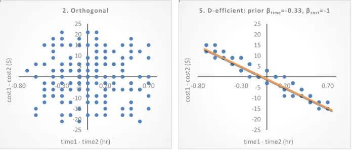
The information contained in each generated design can be plotted graphically as in Figure 1 (where we show the results for design 2 orthogonal and design 5 D-efficient with VOT prior of $20/hour). Each point on this plot represents a choice task in the design, and the location of the point represents the hypothetical travel times and travel costs presented in that choice task. More specifically, the points are plotted as the difference in travel time and cost between the two alternatives in the binary choice set. For example, using the example choice task that was provided in the introduction of ($4, 60 minutes) versus ($10, 30 minutes), this point would be shown on the graph as X = 60 – 30 minutes = 0.5 hours and Y = $4 – $10 = -$6, i.e. the point at (0.5 hours, -$6). Any such choice task in this context can be represented by a point on this graph, although note that the same point on the graph can represent different choice tasks.
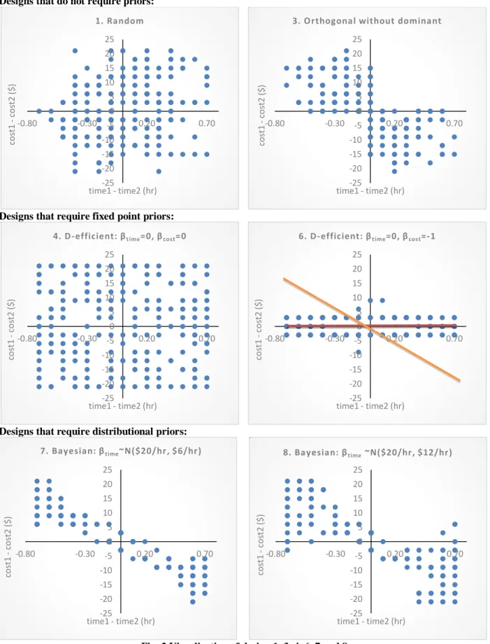
From Figure 1, we see that points in orthogonal design scatter across nearly the whole 2D space, while the D-efficient design points center around the orange line representing the prior assumption of VOT =$20/hour. Fig. 2 presents the visualization for designs 1, 3, 4, 6, 7 and 8 (the remaining one-stage designs), for which we see the same trend: efficient designs (both D-efficient and Bayesian efficient) are tailored much closer around the prior assumption about the parameters (except for the D-efficient design that assumes priors equal to zero), while the random and orthogonal design are much more scattered. This is expected and a result of the theoretical foundation of the designs. The choice contexts in the efficient designs are such that, if the prior were true, the two alternatives presented against each other have nearly equal systematic utilities. These are the choice contexts in which the decision maker has to be most discerning, i.e. it is hardest for him/her to make a choice because the alternatives are nearly balanced. (In Fosgerau and Börjesson, 2015, this area where the respondent has to be most discerning is the 0.4-0.6 probability zone shaded in their Figure 1.) If one thinks of the S-curve choice probability function (X axis is the difference in systematic utilities and Y axis is the probability of choosing alternative 1), these generated choice tasks would be clustered along the region where the curve is steep, i.e. sloping up from probability of zero to probability of 1. On the other hand, having respondents make choices from choice contexts that are closest to the X or Y axis along the S-curve does not provide much information to infer VOT (such points would be along the flatter parts of the S-curve). At the extreme, points in the 2 quadrants where the systematic utility of one alternative
9
dominates the other provide little information on VOT. Under the reasonable assumption that the time and cost parameters are negative, people choose the cheapest AND fastest alternative if such a case is presented to them. In a deterministic model, indeed such dominated choice tasks provide no additional information beyond confirming the signs of the parameters. In a stochastic model, such tasks with dominated alternatives do inform the estimates (e.g, the scale), but relatively minimally. With limited resources, one will gain more information from responses to choice tasks in the trade-off quadrants than in the dominated quadrants. Therefore, there are a lot of “wasted” points in designs such as the orthogonal design which has numerous points in the relatively uninformative quadrants where either alternative 2 is dominant (upper right quadrant) or alternative 1 is dominant (the lower right quadrant). The question is then whether the D-efficient design is able to estimate the true parameters in situations where the priors are highly incorrect. Such a situation is demonstrated with design 6, where the red line is the VOT that was used for the prior in the D-efficient design (time parameter = 0 and cost parameter = -1). Since the red line was used as a prior, the generated choice contexts cluster around this red line. If the true value is the orange line ($20/hour), it appears this design will perform poorly as most of the choice contexts do not provide much information.
As we would expect, these visualizations suggest that the efficient designs (both D-efficient and Bayesian efficient) will perform better if the prior parameters are close to the truth, but also will be more sensitive towards a misspecification of the prior parameters. That said, the Bayesian efficient designs (7 and 8) appear more robust to incorrect priors as the points cover a broader range, even more so with a larger standard deviation (8). The next section explores these expectations empirically.
Fig. 1 Visualization of design 2 and 5
-25 -20 -15 -10 -5 0 5 10 15 20 25 -0.80 -0.30 0.20 0.70 cost 1 - cost 2 ($ ) time1 - time2 (hr) 2. Orthogonal -25 -20 -15 -10 -5 0 5 10 15 20 25 -0.80 -0.30 0.20 0.70 cost 1 - cost 2 ($ ) time1 - time2 (hr)
10
Designs that do not require priors:
Designs that require fixed point priors:
Designs that require distributional priors:
Fig. 2 Visualization of design 1, 3, 4, 6, 7 and 8
-25 -20 -15 -10 -5 0 5 10 15 20 25 -0.80 -0.30 0.20 0.70 cost 1 - cost 2 ($ ) time1 - time2 (hr) 1. Random -25 -20 -15 -10 -5 0 5 10 15 20 25 -0.80 -0.30 0.20 0.70 cost 1 - cost 2 ($ ) time1 - time2 (hr)
3. Orthogonal without dominant
-25 -20 -15 -10 -5 0 5 10 15 20 25 -0.80 -0.30 0.20 0.70 cost 1 - cost 2 ($ ) time1 - time2 (hr)
4. D-efficient: βtime=0, βcost=0
-25 -20 -15 -10 -5 0 5 10 15 20 25 -0.80 -0.30 0.20 0.70 cost 1 - cost 2 ($ ) time1 - time2 (hr) 6. D-efficient: βtime=0, βcost=-1
-25 -20 -15 -10 -5 0 5 10 15 20 25 -0.80 -0.30 0.20 0.70 cost 1 cost 2 ( $) time1 - time2 (hr) 7. Bayesian: βtime~N($20/hr, $6/hr) -25 -20 -15 -10 -5 0 5 10 15 20 25 -0.80 -0.30 0.20 0.70 cost 1 cost 2 ( $ ) time1 - time2 (hr) 8. Bayesian: βtime ~N($20/hr, $12/hr)
11
4 ROBUSTNESS ANALYSIS
In this section, we perform a robustness analysis to see how well the different designs perform under a wide range of true values of time. Recall that we are using the design to collect data to estimate VOT according to equation 4, and recall that the efficient designs were generated based on prior assumptions regarding the true parameter. Presumably, if the prior is $20/hour and the truth is (also) $20/hour, the efficient design will outperform the orthogonal and random designs. The central question here is what happens when the truth is far from the prior. For each of the eight single stage designs (the two-stage designs are described in the next section) we test how each performs for 15 different true VOTs: 0, 1, 2, 5, 10, 15, 20, 30, 40, 50, 60, 70, 80, 90, 100. In order to evaluate the performance of each design we need to measure the efficiency. We do this in 2 ways: an analytical calculation of the D-error and a microsimulation of the standard error.
The analytical computation of the D-error efficiency is equivalent to computing the D-error when creating the efficient designs, see eq. 5-7, but instead of using the prior parameters, we now use the candidates for the true parameters that we want to test.
To calculate the standard error using microsimulation, we relied on synthetic datasets generated by assuming a set of true parameters and simulating choices from a set of simulated respondents. As described above, each design results in 200 choice tasks. We double that to obtain a total of 400 choice responses, i.e. we simulate that each choice task is presented to two (different) individuals. We chose this sample size as being representative of a real (albeit fairly small) VOT study. We assume that the 400 responses are independent. Next, we specify a VOT, e.g. $10/hour, and for each simulated individual we draw two random error terms (one for each alternative) from the Extreme Value type 1 distribution. We then calculate the utility based on the level values in the choice tasks, the drawn error terms, and the assumed (true) VOT. The alternative with the highest utility is then labeled the chosen alternative for that simulated individual. We perform this simulation 100 times with new random draws for the error terms. We estimate the model for each of the 100 synthetic datasets, and for each obtain the estimated VOT. As the simulated measure of robustness, we calculate the standard deviation among the estimated VOTs for each given true VOT and experimental design combination. This process is repeated for all eight designs for each of the 15 different true VOTs.
It’s important to note that while we focus on efficiency throughout this paper, we did confirm that (as intended) all of our estimates from the random and orthogonal designs produce unbiased estimates for the entire range of VOT that was tested. We also can confirm that the efficient designs also produced unbiased estimates for a broad range of VOTs tested. However, for high values of times (>$60/hour for D-efficient and >$80 for Bayesian D-efficient) we could not demonstrate the unbiasedness for the efficient designs due to the very large standard errors. The issue is that the choice task selection process in the efficient designs results in a lack of choice tasks presented with trade-offs in the vicinity of the true value of time (when it was significantly higher than the prior used to generate the design). In a deterministic model, such efficient design would not yield a unique estimate as the VOTs within this unobserved range would result in equal fit to the data. In a stochastic model, the VOT is identified but with extremely large standard errors such that unbiasedness could not be demonstrated with a finite sample. Further, unlike Bliemer et al (2015), we do not find evidence in our simulation that bias is introduced by either inclusion or by exclusion of the dominant alternatives; designs 1 and 2 include dominant alternatives while design 3 excludes dominant alternatives, and all three designs lead to unbiased estimates of VOT across our range of tested VOTs. The results of these robustness tests are shown in Figures 3 and 4. Due to space, we only plot the D-error results, but the microsimulation results are comparable although not quite as smooth due to simulation error. One additional aspect that the microsimulation provides is that the standard error is in the units of the VOT and is a function of the number of responses, so it provides a nice reference point of the magnitudes of the differences (rather than the unit-less D-error). We provide these units along the right vertical axis as an approximation since the graphs are not exactly identical. Figure 3 presents the results for true VOTs from $10/hour to $30/hour – and centered on $20/hour, the basis of most of our priors. With the exception of design 6, the designs perform similarly in this range. Design 6 was generated by assuming a prior of 0 for the time parameter and a prior of -1 for the cost parameter. It is not surprising this design performs poorly over most of the range given the plot in Figure 2, and performs best near $0/hour (which is its prior). The efficient designs based on the $20/hour prior (designs 5, 7, and 8) perform best
12
Fig. 3 Robustness results focusing on region around prior VOT of $20/hour
0.0 0.5 1.0 1.5 2.0 2.5 0.000 0.005 0.010 0.015 0.020 0.025 10 12 14 16 18 20 22 24 26 28 30 A ppr o xi m at e Sta nda rd Er ro r o f V O T pa ram eter ($ /hr ) f o r 40 0 o bs er vat io ns D -er ro r (uni tl es s) True VOT ($/hr) (1) Random design (2) Orthogonal design
(3) Orthogonal design without dominant alternatives (4) D-efficient: β_time=0, β_cost=0, VOT: undefined (5) D-efficient: β_time=-0.33, β_cost=-1, VOT=$20/hour (6) D-efficient: β_time=0, β_cost=-1, VOT=$0/hour
(7) Bayesian: β_time~Normal($20/hour, $6/hour), β_cost=-1 (8) Bayesian: β_time~Normal($20/hour, $12/hour), β_cost=-1
13
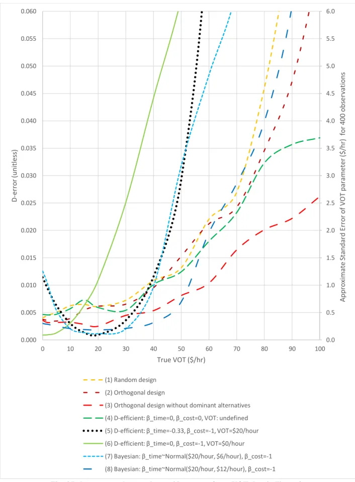
Fig. 4 Robustness results covering a wider range of true VOT than in Figure 3
0.0 0.5 1.0 1.5 2.0 2.5 3.0 3.5 4.0 4.5 5.0 5.5 6.0 0.000 0.005 0.010 0.015 0.020 0.025 0.030 0.035 0.040 0.045 0.050 0.055 0.060 0 10 20 30 40 50 60 70 80 90 100 A ppr o xi m at e Sta nda rd Er ro r o f V O T pa ram eter ($ /hr ) f o r 40 0 o bs er vat io ns D -er ro r (uni tl es s) True VOT ($/hr) (1) Random design (2) Orthogonal design
(3) Orthogonal design without dominant alternatives (4) D-efficient: β_time=0, β_cost=0, VOT: undefined (5) D-efficient: β_time=-0.33, β_cost=-1, VOT=$20/hour (6) D-efficient: β_time=0, β_cost=-1, VOT=$0/hour
(7) Bayesian: β_time~Normal($20/hour, $6/hour), β_cost=-1 (8) Bayesian: β_time~Normal($20/hour, $12/hour), β_cost=-1
14
across most of this range but begin to degrade at the edges. The three designs that cover the 2D space (1, 2, and 4) perform similarly. Design 3, which is the orthogonal with dominated choice tasks removed, performs better than 1, 2 and 4 and is closer to the efficient designs. This suggests that cleaning out the dominated choice tasks does a lot to achieve the efficiency gains of an efficient design. It also supports our earlier statement that choice tasks in the dominant quadrants would be better spent if shifted to choice tasks in the trade-off quadrants. (Also note that we found no evidence that either including or excluding dominated choice tasks lead to bias as suggested in Bliemer et al., 2015. The caveat, which may add some insight into that work, is that we did find that the points on the X and Y axis—which have dominant alternatives—did need to be included in order to obtain unbiased estimates.)
The conclusions from Figure 3 are comparable to what has been produced in the literature (e.g., Rose and Bliemer, 2009) in that the efficient designs appear to perform better across a range of true values although begin to degrade at the edges. In which case, the range of the X-axis of the plot becomes critical to evaluating the designs. This also points to the power of our setup that plots the results for clear units of VOT, rather than the fairly meaningless units from a single parameter (such as util/$ for a cost parameter) or an abstract setup where the explanatory variables have no meaningful units. Indeed, when we plot the same data in Figure 3 across a wider VOT range as shown in Figure 4, we draw very different conclusions. We saw an inkling of the efficient designs degrading in Figure 3, and here it becomes much more pronounced. Design 5 (D-efficient with $20/hour as prior) and design 7 (Bayesian with smaller variance) perform similarly and begin to rapidly deteriorate around $50/hour. Increasing the variance in the Bayesian design (design 8) extends this breakdown point out to around $80/hour, which is similar to where the random and orthogonal designs rapidly deteriorate. Interestingly, the D-efficient design with naïve priors (design 4 with priors set to 0) follows the orthogonal and random designs for most of the range, but then performs better at the higher values of $90/hour and $100/hour. Looking at Figure 1, this is explained by the fact that the D-efficient design with naïve priors more uniformly covers the extremities of the 2D space. The design that is most robust for high VOTs (i.e. above $50/hour) is the cleaned orthogonal design (3). This makes sense as this design covers a wide range of VOT, but does not “waste” observations on dominated choice tasks, which reveal little about the trade-off. The cleaned orthogonal design seems to be the overall best performer of those we tested, but such cleaning would help any design.
5 VARIATIONS ON A THEME: 2 STAGE DESIGNS
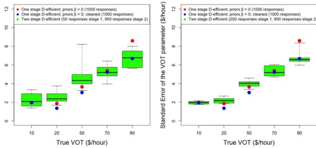
To address the issue of needing to have estimates of the parameters before creating efficient designs, a relatively common practice is to conduct a 2-stage survey design. In the first stage, a design with naïve priors is used to collect a small sample in order to estimate initial values of the parameters. These initial values are then used in the second stage as priors to create an efficient design, which is then applied to a larger sample to generate the final estimation results. Either fixed values from the first stage can be used to produce a D-efficient design in the second stage, or the distribution of the estimate (point estimate and standard error with normal distribution) can be used to produce a Bayesian efficient design. We analyzed both of these cases, and the results are shown in Fig. 5. The key metric reported is the microsimulated standard error of the VOT estimate. For this scenario, we assume there are resources for a total of 1000 respondents and that a subset of this sample may be used in the first stage to estimate priors for the second stage. The top row reports the D-efficient results, where the left figure has a smaller stage 1 sample (50 responses) and the right figure has a larger stage 1 sample (200 responses). The bottom row reports the Bayesian efficient design with the same assumptions on the size of the first stage. For comparison, the microsimulated standard errors for the naïve D-efficient one-stage samples where all 1000 responses are used in the first stage are also reported: the red dot is for a D-efficient design with priors set to 0 (equivalent to design 4 in Fig. 2) and the blue dot is also D-efficient with priors set to 0, except that all responses in the dominant quadrants (upper right and lower left) are removed. The 2-stage results have a distribution because the parameters produced in the first stage are a random variable. Fig. 5 was produced by doing 10 different runs for each case.
The conclusion from this single example is that the 2-stage results do not appear to be more robust than the naïve 1-stage results. While the Bayesian second 1-stage outperforms the D-efficient second 1-stage in terms of lower standard errors and less variability, the naïve 1-stage model (particularly the cleaned version) outperforms the 2-stage approach for moderate true values of time. Results will of course vary based on the specific context, and may be particularly sensitive to the variance of the error.
15
(a) Two stage with 50 responses used in stage 1 (b) Two stage with 200 responses used in stage 1 to generate priors for a D-efficient design to generate priors for a D-efficient design
to be applied to 950 responses in stage 2. to be applied to 800 responses in stage 2.
(c) Two stage with 50 responses used in stage 1 (d) Two stage with 200 responses used in stage 1 to generate priors for a Bayesian D-efficient design to generate priors for a Bayesian D-efficient design to be applied to 950 responses in stage 2. to be applied to 800 responses in stage 2.
16
6 REAL DESIGN EXPERIMENT
To build on the previous analysis, we test our results using a more complex context of departure time choice. This is the experiment that motivated the investigation presented in this paper. For the original experiment, significant effort was expended to generate an efficient design. The model specification led to a particularly complex design, and it resulted in potentially important explanatory variables being excluded from the choice tasks. Further, the design was generated based on a relatively simple, homogeneous logit formulation; and then the dataset produced was used to estimate far more complex, heterogeneous models. This lead us to explore the potential value of the efficient design approach in the relatively more straightforward setting described in the paper thus far. Now we return to our motivating case to explore the ideas in a more complex context.
The objective of the experiment was to study departure time choices in the capital region of Denmark, i.e. the Greater Copenhagen Area. The stated choice experiment was built specifically for the scheduling model (Small, 1982):
Vint= ASC𝑖+ βTT∙ TTint+ βTC∙ TCint+ βSDE∙ SDEint+ βSDL∙ SDLint, (8) where:
SDEint= max(−SDint; 0), (9)
SDLint= max(0; SDint), and (10)
SDint= ATint− PAT𝑛 . (11)
Vint is the systematic utility for alternative i, individual n and choice task t. It is a function of the alternative specific constant (ASC), the attributes travel time (TT), travel cost (TC), scheduling delay early (SDE), and scheduling delay late (SDL), and their corresponding parameters to be estimated. Note that the scheduling delay (SD) is divided into two parts (i.e. being early or being late), and it is calculated as the difference between actual arrival time (AT) and preferred arrival time (PAT) at work.
The design was built with three departure time options, and all attributes were defined by three level values, except TC which had four levels. The design was constructed using a D-efficient design, and the prior parameters were defined based on the existing literature. The priors used to generate the final design are β̃𝑇𝑇= -0.012, β̃TC= -0.018, β̃SDL= -0.008, and β̃SDL= -0.012. Six different designs were built based on different travel time durations (ranging from 10-60 minutes) but otherwise are identical. The respondents were then assigned to the design which best resembles their actual trip to work. We did this in order to mimic a real life situation as realistically as possible. Note that each of the six designs was constructed with a total of 27 choice tasks (divided into three blocks with 9 choice tasks). For a detailed description of the stated choice experimental design see Thorhauge et al. (2014).
As in the controlled experiment, the aim is to see how the design performs when the true parameter is close and far away from the prior parameters used to build the efficient design. To test the robustness of the design, we relied on microsimulation to generate synthetic datasets. More specifically, we collapsed all six designs into one experimental design consisting of 162 choice tasks in order to cover the entire range of choice tasks, and then we assumed that each choice task was presented to 100 individuals, hence a total of 16,200 observations. We assumed a set of true parameters and simulated the choice by drawing random numbers from the EV type 1 distribution for each observation and alternative. We generated 100 synthetic datasets and calculated the average standard error across the 100 estimations. We repeated the process for true parameters ranging from 10 times smaller than the prior to 10 times larger with a step size equal to 1/10 of the prior parameter and we tested a total of 100 different values of the true parameter. We performed this test for each of the four variables separately and kept the remaining three constant.
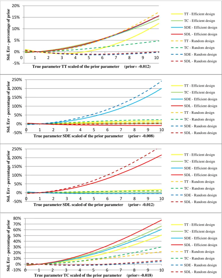
For comparison, we also created a random factorial design and simulated it in the same way. Figure 6 shows how the (average) standard errors change (with respect to the standard error when using the prior parameter values as the true parameter) when the true parameter changes for both the efficient and random design.
The design is able to recover the true parameters even when it is different from the prior parameters. However, as the difference between the prior and the true parameter increases, the standard error increases and many model estimations are unidentified. This indicates a poorly performing design not built to estimate true parameters far from the prior parameters. The design seems to be more sensitive to changes in TC and especially SDL and SDE (the standard error increases by 200%, see Figure 6). However, when changing the true parameter of ETT, the lowest
17
Fig. 6 Standard error in percent with respect to the standard error of the prior as function of scaled true parameters
-5% 0% 5% 10% 15% 20% 0 1 2 3 4 5 6 7 8 9 10 S td . E rr p er ce n tage o f p ri o r
True parameter TT scaled of the prior parameter (prior= -0.012)
TT - Efficient design TC - Efficient design SDE - Efficient design SDL - Efficient design TT - Random design TC - Random design SDE - Random design SDL - Random design -50% 0% 50% 100% 150% 200% 250% 0 1 2 3 4 5 6 7 8 9 10 S td . E rr p er ce n tage o f p ri o r
True parameter SDE scaled of the prior parameter (prior= -0.008)
TT - Efficient design TC - Efficient design SDE - Efficient design SDL - Efficient design TT - Random design TC - Random design SDE - Random design SDL - Random design -50% 0% 50% 100% 150% 200% 250% 0 1 2 3 4 5 6 7 8 9 10 S td . E rr p er ce n tage o f p ri o r
True parameter SDL scaled of the prior parameter (prior= -0.012)
TT - Efficient design TC - Efficient design SDE - Efficient design SDL - Efficient design TT - Random design TC - Random design SDE - Random design SDL - Random design -10% 0% 10% 20% 30% 40% 50% 60% 70% 80% 0 1 2 3 4 5 6 7 8 9 10 S td . E rr p er ce n tage o f p ri o r
True parameter TC scaled of the prior parameter (prior= -0.018)
TT - Efficient design TC - Efficient design SDE - Efficient design SDL - Efficient design TT - Random design TC - Random design SDE - Random design SDL - Random design
18
standard error does not occur at the value of the prior but instead at a true parameter that is 2.8 times higher than the prior. Comparing this design with the random design, we see that the performances are rather close when varying the true parameter for SDE and SDL. As we increase the true parameter for TC we see that all parameters in the efficient designs have higher standard errors. We see the same picture when we increase the true parameter for TT, except for one of the parameters. Overall, we see tendencies that could verify the findings in our controlled experiment, but more research is needed as many factors can influence performance in a complex non-controlled experiment.
7 CONCUSIONS
There is a substantial amount of literature demonstrating the efficiency improvements of employing efficient designs when the priors used to generate the efficient designs are assumed to be accurate. Far less literature exists that compares how different design types perform for different values of the true parameters. Our paper analyzes the robustness of different designs within a typical stated choice experiment context of a trade-off between price and quality. The key parameter to estimate is the value of time (VOT), and we test many designs to examine how robust efficient designs are against a misspecification of the prior parameters. Our experimental design is such to ensure consistent estimates so that we can focus on efficiency as our robustness metric. Our analysis builds on previous literature by using an extremely simple experimental setup in order to provide insightful visualizations of the designs and an interpretable reference point (VOT) for the range in which the design is robust. Our findings indicate that efficient experimental design is a good first choice if one is confident in the prior parameters that are to be estimated. However, it is risky to use an efficient design with uncertain priors. In our example, the D-efficient design is most efficient in the region where the true population VOT is near the prior used to generate the design: the prior is $20/hour and the efficient range is $10/hour -$30/hour. However, the D-efficient design quickly becomes the most inefficient outside of this range (under $5/hour and above $40/hour), and the estimation significantly degrades above $50/hour. Bayesian efficient designs are more robust than D-efficient designs since they take uncertainty into account, although in our simple example the Bayesian designs also degraded above $80/hour even with a seemingly large variance used for the prior (and degraded above $50/hour with a smaller variance). Introducing a 2-stage design where a small sample is used to generate priors also did not prove to produce robust estimates across a large range of VOT. Interestingly, 2-stage designs did better for extreme values of time, however, naïve designs did better for moderate values of time. While we assume a heterogeneous population throughout, results for a heterogeneous population could exacerbate the limitations of the less robust models as it is more likely that portions of the population fall outside of the robust range of parameter values. Arguably, the random design (which is the easiest to generate) performs as well as any design, and it (as well as any design) will perform even better if data cleaning is done to remove choice tasks where one alternative dominates the other. While our example is a simplified one, real applications are rarely so simple; models are often highly complex with numerous parameters and significant heterogeneity (both systematic and random), as demonstrated in our real design experiment. Further research is needed as many factors influence performance. In the meantime, our results suggest that efficient designs only be used when we have excellent priors, and this paper serves as a reference to support the use of non-efficient design methods in stated choice experiments.
ACKNOWLEDGEMENTS
An earlier draft of this work was initially presented at the Transportation Research Board annual meeting in January of 2015 (Walker et al., 2015), and we thank the reviewers from that process as well as the discussion that followed from the presentation and circulation of the working paper. We thank Andre de Palma and Nathalie Picard for organizing the symposium in honor of Daniel McFadden and for following it up with this special issue. We thank two anonymous reviewers assigned by this journal. We also thank Michael Galczynski for the idea for the title.
19
REFERENCES
Adamowicz, W., Louviere, J. & Williams, M., 1994, Combining Revealed and Stated Preference Methods For Valuing Environmental Amenities, Academic Press Inc JNL-Comp Subscriptions.
Belenky, P., 2011, Revised Departmental Guidance on Valuation of Travel Time in Economic Analysis (Revision 2), U.S. Department of Transportation, Washington DC.
Bliemer, M.C.J. & Collins, A.T., 2016, On determining priors for the generation of efficient stated choice experimental designs, The Journal of Choice Modelling, 21, 10-14.
Bliemer, M.C.J. & Rose, J.M., 2010a, "Serial Choice Conjoint Analysis for Estimating Discrete Choice Models" in Choice Modelling: The State-of-the-art and the State-of-practice (Proceedings from the inaugural International Choice Modelling Conference), eds. S. Hess & A. Daly, Emerald Group Publishing, Bingley, UK, 139-161. Bliemer, M.C.J. & Rose, J.M., 2010b, Construction of experimental designs for mixed logit models allowing for
correlation across choice observations, Transportation Research Part B: Methodological, 6, 720-734.
Bliemer, M.C.J. & Rose, J.M., 2011, Experimental design influences on stated choice outputs: An empirical study in air travel choice, Transportation Research Part A: Policy and Practice, 1, 63-79.
Bliemer, M.C.J., Rose, J.M. & Chorus, C.G., 2017, Detecting dominance in stated choice data and accounting for dominance-based scale differences in logit models, Transportation Research Part B: Methodological, 201, 83-104.
Bliemer, M.C.J., Rose, J.M. & Hensher, D.A., 2009, Efficient stated choice experiments for estimating nested logit models, Transportation Research Part B: Methodological, 1, 19-35.
Bliemer, M.C.J., Rose, J.M. & Hess, S., 2008, Approximation of Bayesian efficiency in experimental choice designs, Journal of Choice Modelling, 1, 98-126.
Bradley, M. & Bowy, P.H.L., 1984, A stated preference analysis of bicyclist route choice, PTRC, Summer Annual Meeting, Sussex, 39-53.
Burgess, L. & Street, D.J., 2005, Optimal designs for choice experiments with asymmetric attributes, Journal of Statistical Planning and Inference, 1, 288-301.
ChoiceMetrics, 2012a, Ngene 1.1.1 User Manual & Rerence Guide, ChoiceMetrics.
ChoiceMetrics, 2012b, Ngene software, version: 1.1.1, Build: 305, developed by Rose, John M.; Collins, Andrew T.; Bliemer, Michiel C.J.; Hensher, David A.
Cummings, R.G., Brookshire, D.S. & Schulze, W.D. (eds) 1986, Valuing Environmental Goods: A state of the Arts Assessment of the Contingent Method, Rowman and Allanheld, Totowa, NJ.
Davidson, J.D., 1973, Forecasting Traffic on STOL, Oper Res Q, 4, 561-569.
Fosgerau, M. & Börjesson, M., 2015, Manipulating a stated choice experiment. Journal of Choice Modelling, 16, 43-49.
Fowkes, A.S., 2000, "Recent developments in state preference techniques in transport research" in Stated Preference Modelling Techniques, ed. J.d.D. Ortúzar, PTRC Education and Research Services, London, 37-52.
Hensher, D.A. & Louviere, J.J., 1983, Identifying Individual Preferences For International Air Fares - An Application Of Functional-Measurement Theory, Univ Bath.
Hensher, D.A., 1982, Functional-Measurement, Individual Preference And Discrete-Choice Modeling - Theory And Application, Journal of Economic Psychology, 4, 323-335.
Hensher, D.A., 1994, Stated Preference Analysis Of Travel Choices - The State Of Practice, Kluwer Academic Publ. Johnson, F.R., Kanninen, B., Bingham, M. & Özdemir, S., 2007, "Experimental Design for Stated Choice Studies"
in Valuing Environmental Amenities Using Stated Choice Studies, ed. B.J. Kanninen, Springer, Dordrecht, 159-202.
Johnson, F.R., Lancsar, E., Marshall, D., Kilambi, V., Muehlbacher, A., Regier, D.A., Bresnahan, B.W., Kanninen, B. & Bridges, J.F.P., 2013, Constructing Experimental Designs for Discrete-Choice Experiments: Report of the ISPOR Conjoint Analysis Experimental Design Good Research Practices Task Force, Value in Health, 1, 3-13. Kanninen, B.J., 2002, Optimal design for multinomial choice experiments, Journal of Marketing Research, 2,
214-227.
Kocur, G., Adler, T., Hyman, W. & Audet, E., 1982, Guide to Forecasting Travel Demand with Direct Utility Measurement, UMTA, USA Department of Transportation, Washington D.C.
Kuhfeld, W.F., Tobias, R.D. & Garratt, M., 1994, Efficient Experimental Design with Marketing Research Applications, Journal of Marketing Research (JMR), 4.
Louviere, J.J. & Hensher, D., 1982, Design And Analysis Of Simulated Choice Or Allocation Experiments In Travel Choice Modeling, Transportation Research Record, 11-17.
20
Louviere, J.J. & Hensher, D.A., 1983, Using Discrete Choice Models With Experimental-Design Data To Forecast Consumer Demand For A Unique Cultural Event, Journal of Consumer Research, 3, 348-361.
Louviere, J.J. & Kocur, G., 1983, The magnitude of individual-level variations in demand coefficients: a Xenia, Ohio case example, Transportation Research, Part A, 5, 363-373.
Louviere, J.J. & Woodworth, G., 1983, Design and Analysis Of Simulated Consumer Choice Or Allocation Experiments - An Approach Based On Aggregate Data, Journal of Marketing Research, 4, 350-367. Louviere, J.J., Meyer, R., Stetzer, F. & Beavers, L.L., 1973, Theory, methodology and findings in mode choice
behavior, Working Paper No., The Institute of Urban and Regional Research, The University of Iowa, Iowa City.
Mitchell, R.C. & Carson, R.T. (eds) 1989, Using Surveys to Value Public-Goods - The Contingent Valuation Method, John Hopkins Univ. Press for Resources for the Future, Baltimore, MD.
Ojeda-Cabral, M., Hess, S. & Batley, R., 2016, Understanding valuation of travel time changes: are preferences different under different stated choice design settings? Transportation, 1-21.
Rose, J.M. & Bliemer, M.C.J., 2008, "Stated preference experimental design strategies" in Handbook in Transport, vol. 1, eds. D.A. Hensher & K. Button, second edn, Elsevier Science, Oxford.
Rose, J.M. & Bliemer, M.C.J., 2009, Constructing Efficient Stated Choice Experimental Designs, Transport Reviews, 5, 587-617.
Rose, J.M. & Bliemer, M.C.J., 2013, Sample size requirements for stated choice experiments, Transportation, vol. 40, 5, 1021-1041.
Rose, J.M. & Bliemer, M.C.J., 2014, "Stated choice experimental design theory: the who, the what and the why” in Handbook of Choice Modelling, eds. S. Hess & A. Daly, Edward Elgar Publishing, ch. 7, 152–177.Rose, J.M., Bliemer, M.C.J., Hensher, D.A. & Collins, A.T., 2008, Designing efficient stated choice experiments in the presence of reference alternatives, Transportation Research Part B, 4, 395-406.
Sándor, Z. & Wedel, M., 2001, Designing Conjoint Choice Experiments Using Managers' Prior Beliefs, Journal of Marketing Research, 4.
Sándor, Z., Wedel, M., 2002, Profile construction in experimental choice designs for mixed logit models, Marketing. Science, vol. 21, 4, 455-475.Small, K.A., 1982, The Scheduling of Consumer Activities: Work Trips, American Economic Review, 3, 467–479.
Street, D.J. & Burgess, L., 2004, Optimal and near-optimal pairs for the estimation of effects in 2-level choice experiments, Journal Of Statistical Planning And Inference, 1-2, 185-199.
Street, D.J., Bunch, D.S. & Moore, B.J., 2001, Optimal designs for 2k paired comparison experiments, Communications in Statistics - Theory and Methods, 10, 2149-2171.
Street, D.J., Burgess, L. & Louviere, J.J., 2005, Quick and easy choice sets: Constructing optimal and nearly optimal stated choice experiments, International Journal Of Research In Marketing, 4, 459-470.
Thorhauge, M., Cherchi, E. & Rich, J., 2014, Building efficient stated choice design for departure time choices using the scheduling model: Theoretical considerations and practical implications, Working paper.
Thorhauge, M., Cherchi, E. & Rich, J., 2016a, How Flexible is Flexible? Accounting for the Effect of Rescheduling Possibilities in Choice of Departure Time for Work Trips. Transportation Research Part A: Practice and Policy, 86, 177-193.
Thorhauge, M., Haustein, S. & Cherchi, E., 2016b, Social Psychology Meets Microeconometrics: Accounting for the Theory of Planned Behaviour in Departure Time Choice. Transportation Research Part F: Traffic Psychology and Behaviour, 38, 94-105.
Toner, J.P., Clark, S.D., Grant-Muller, S. & Fowkes, A.S., 1999, Anything you can do, we can do better: A provocative introduction to a new approach to stated preference design, World Transport Research, VOLS 1-4. Walker, J.L., Wang, Y., Mikkel, T., & Ben-Akiva, E., 2015, D-EFFICIENT OR DEFICIENT? A Robustness
Analysis of Stated Choice Experimental Designs, presented at the 94th annual meeting of the Transportation Research Board, Washington, D.C.