HAL Id: hal-01938713
https://hal.inria.fr/hal-01938713
Submitted on 28 Nov 2018
HAL is a multi-disciplinary open access
archive for the deposit and dissemination of
sci-entific research documents, whether they are
pub-lished or not. The documents may come from
teaching and research institutions in France or
abroad, or from public or private research centers.
L’archive ouverte pluridisciplinaire HAL, est
destinée au dépôt et à la diffusion de documents
scientifiques de niveau recherche, publiés ou non,
émanant des établissements d’enseignement et de
recherche français ou étrangers, des laboratoires
publics ou privés.
balancedness, efficiency
Luca Arpaia, Mario Ricchiuto
To cite this version:
Luca Arpaia, Mario Ricchiuto. r–adaptation for Shallow Water flows: conservation, well balancedness,
efficiency. Computers and Fluids, Elsevier, 2018, 160, pp.175 - 203. �10.1016/j.compfluid.2017.10.026�.
�hal-01938713�
r−adaptation for Shallow Water flows:
conservation, well balancedness, efficiency
Luca Arpaia* and Mario Ricchiuto*
*Team CARDAMOM
Inria Bordeaux Sud-Ouest
conservation, well balancedness, efficiency
Luca Arpaia and Mario Ricchiuto
early draft
Abstract
We investigate the potential of the so-called ”relocation” mesh adaptation in terms of resolu-tion and efficiency for the simularesolu-tion of free surface flows in the near shore region. Our work is developed in three main steps. First, we consider several Arbitrary Lagrangian Eulerian (ALE) formulations of the shallow water equations on moving grids, and provide discrete analogs in the Finite Volume and Residual Distribution framework. The compliance to all the physical constraints, often in competition, is taken into account. We consider di↵erent formulations allowing to combine volume conservation (DGCL) and equilibrium (Well-Balancedness), and we clarify the relations between the so-called pre-balanced form of the equations (Rogers et al., J.Comput.Phys. 192, 2003), and the classical upwiniding of the bathymetry term gradients (Bermudez and Vazquez, Computers and Fluids 235, 1994). Moreover, we propose a simple remap of the bathymetry based on high accurate quadrature on the moving mesh which, while preserving an accurate representation of the initial data, also allows to retain mass conserva-tion within an arbitrary accuracy. Second, the coupling of the resulting schemes with a mesh partial di↵erential equation is studied. Since the flow solver is based on genuinely explicit time stepping, we investigate the efficiency of three coupling strategies in terms of cost over-head w.r.t. the flow solver. We analyze the role of the solution remap necessary to evaluate the error monitor controlling the adaptation, and propose simplified formulations allowing a reduction in computational cost. The resulting ALE algorithm is compared with the rezoning Eulerian approach with interpolation proposed e.g. in (Tang and Tang, SINUM 41, 2003). An alternative cost e↵ective Eulerian approach, still allowing a full decoupling between adapta-tion and flow evoluadapta-tion steps is also proposed. Finally, a thorough numerical evaluaadapta-tion of the methods discussed is performed. Numerical results on propagation, and inundation problems shows that the best compromise between accuracy and CPU time is provided by a full ALE formulation. If a loose coupling with the mesh adaptation is sought, then the cheaper Eulerian approach proposed is shown to provide results quite close to the ALE.
1
Introduction
We investigate the potential benefits of r-adaptation techniques (or relocation adaptation) in the computa-tion of propagacomputa-tion and interaccomputa-tion of free surface waves, including their runup on complex bathymetries. The main building blocks of our study are the following. First, we use the well known Shallow Water equations to model the hydrostatic free surface hydrodynamics in vicinity of the shore. The use of moving meshes will lead us to investigate various forms of the model equations in an Arbitrary-Lagrangian-Eulerian (ALE) setting. Particular attention is paid to the respect of all the physical constraints. Second, the equa-tions are coupled with a Laplacian-based adaptive mesh deformation technique. The coupling between
flow evolution and mesh Partial Di↵erential Equation (PDE) is discussed. Third, a thorough quantita-tive evaluation of the resulting algorithms on benchmarks involving wave propagation and inundation of complex bathymetries is performed.
The numerical approximation of Shallow Water flows is still a subject of intense research. For our purposes, the most interesting issue is the need of preserving, possibly to machine accuracy, the so-called lake at rest steady state. This property is known as C-property or well balacedness (WB). The initial work of [1] on the construction of well-balanced Finite-Volume approximations in one dimension, has been led throughout the years to many di↵erent results allowing the construction of unstructured mesh discretizations verifying the C-property via an appropriate coupling of the numerical flux and numerical source terms [2, 3], or based on di↵erent forms of the equations, as the well-balanced form of [4, 5, 6], or the so-called pre-balanced form of Rogers et al. [7, 8, 9]. These ideas have been also incorporated in Finite Element, Residual Distribution, and Discontinuous Galerkin methods (see e.g. [10, 11, 12, 13, 14] and references therein).
To enhance the resolution of complex wave patterns, and of the wetting/drying dynamics we study the use of mesh adaptation techniques based on nodes redistribution (or relocation). These are known as r-adaptation techniques. The reason for this choice is, on one hand the overhead represented by remeshing techniques [15, 16] w.r.t. a single time step of a fully explicit discretization of the shallow water model, on the other the potential shown in the past for these techniques in e.g. [17], and in the numerous works of Budd and collaborators (see e.g. the review [18] and references therein). Nodal movement is obtained by solving an appropriate Moving Mesh Partial Di↵erential Equation (MMPDE). Originally, the equations for grid movement were developed using the visual analogy between potential solutions and curvilinear grids, thus solving, as for the flow potential, a Laplace equation for some reference/computational coordinates X on the actual/physical grid x. In case of solution-driven adaptation a forcing term is added to take into account the regularity of the solution, and usually defined through a monitor function, see [19] for a thorough derivation. Equidistribution of the monitor function is nowday a standard way to achieve an optimal mesh. The central idea is to find a transformation x = M (X, t) that equidistributes the monitor function on the reference domain. During the last decades theoretical arguments and experience lead to the design of quite general monitor functions which can ensure the adaptation to particular features of the solution; the arclenght-type monitor function of Winslow [20], based on solution gradients, is one of the most successful. Ceniceros and Hou [21], for example, used the temperature gradient in the computation of small scales blow up in Boussinesq convection. Budd, Callen and Walsh [22] compared arclength of the potential temperature with a di↵erent monitor function, based on potential vorticity, for the resolution of weather front formation. In more recent years, Huang [23] studied matrix valued monitor functions which can provide both control on mesh size and shape/orientation. A variational formulation of the equidistribution principle allows to take into account specific mesh quality measures such as orthogonality and smoothness, see here the pioneering work of Brackbill and Saltzman [24]. To further enhance the mesh quality, node insertion/deletion can be performed by appropriate local remeshing strategies. These, however, required much higher overheads and more complex data structures, compared to a single step of an explicit discretization of the flow PDEs, and are not considered here. For recent examples the interested reader may refer to [15, 16].
The coupling of the flow solver with the mesh at each time step is non-trivial, as the mesh equations depend on the solution on the (unknown) adapted mesh. In particular the Shallow Water equations and the MMPDE can be either solved simultaneously or alternately. The latter has been successfully implemented by [21], showing a significant reduction of sti↵ness problems even if it can lead to a lag in the mesh movement with respect to the physical features. Depending on the framework in which we evolve the PDE, two di↵erent alternate algorithms are tested at this point. If the PDE is written in Eulerian framework one get the rezoning method suggested in [17]. This approach, based on a sequence of mesh and flow iterations, uses the mesh solver as a black box, the flow equations being solved on a (di↵erent) fixed mesh at each time iteration. Its drawback is that, at each time iteration, the flow solver requires a remap/interpolation on the new mesh which may be quite expensive as it needs to guarantee the same properties as the flow solver itself (high order accuracy, non-oscillatory character/positivity preservation, C-property, mass conservation). At the opposite, once the grid has been adapted, one can evolve the flow with an Arbitrary-Lagrangian-Eulerian formulation of the equations, as suggested e.g. in [25]. In this case,
the properties of the flow solutions are only determined by the scheme. However, a proper ALE form of the numerical discretization has to be used. In particular, a well known requirement for ALE discretizations is the compatibility with a Geometric Conservation Law (GCL), which guarantees that no artificial volume (viz mass) is produced in the computational domain due to mesh motion. The discrete counterpart of this property is known as the DGCL (cf. [26], [27] for an overview). Ideally, in Shallow Water flows, we have to ensure the satisfaction of both a discrete analog of the GCL, and of the C-property, while still being able to conserve mass and momentum. A solution based on an ALE remap of the bathymetry has been suggested in [28]. However, unless such remap is very high order accurate, this quickly leads to a smoothing of the data, hence a re-initialization of the topography is required, spoiling mass conservation.
In this paper, we propose and evaluate simplified strategies allowing adaptive simulations of Shallow Water flows with wetting/drying fronts. In order to do this, we systematically review the forms of the equations which are best suited for the task of combining well-balancedness and DGCL on moving meshes; we use the resulting model equations to provide well-balanced high-order Finite Volume (FV) and Residual Distribution (RD) discretizations, clarifying the relations between the pre-balanced and well-balanced approaches; we provide a simple recipe to marry mass conservation and C-property on moving meshes using a re-interpolation of the nodal bathymetry based on accurate quadrature of the given bathymetric data; we define improved ad-hoc error estimators allowing to better track both smooth waves, and shorelines; finally, coupling strategies allowing cheaper and simpler interpolation algorithms in the adaptation phase, while retaining all the desired discrete properties, are evaluated in terms of CPU time for a given resolution, using standard benchmarks for near shore hydrodynamics.
The paper is organized as follows: section §2 presents the general setting, and it particular it recalls the main forms and properties of the Shallow Water equations, and of a simpler scalar model used to simplify part of the discussion. The well-balanced numerical approximation of the PDEs in ALE form with Finite Volume and Residual distribution schemes is discussed in section§3, with a discussion of the appropriate ALE form for balance laws. The moving mesh algorithm is presented in section §4, with some details concerning the management of wet-dry areas in shallow water simulations. In section §4.2 the interpolation strategy of [29] is presented as a conservative ALE remap. Three strategies to couple mesh movement and balance laws solution are presented in section section§5: the rezoning algorithm of Tang coupled with the SW equations, see Zhou [29] (EUL1), an improved version of the above algorithm (EUL2) and the ALE coupling. Finally, section§7 and section §8 presents a thorough study of the coupled algorithms in terms of accuracy, and CPU time for both simple academic problems and for some classical benchmarks involving the long wave runup on complex bathymetries. The paper is ended by a summary of the main results, and by an overlook at future developments.
2
Problem setting and model equations
2.1
Shallow Water equations and lake at rest
Our final objective is the simulation of the propagation and runup of free surface waves in the near shore region. A good model for the physics of these waves is given by the nonlinear Shallow Water equations, providing a depth averaged description of the flow, and reading
@u
@t +r · f(u) + S(u, b) = 0 , x2 ⌦ (1) where the conserved variables, flux function and source term are given by
u = 2 6 6 6 4 h hu hv 3 7 7 7 5, f (u) = 2 6 6 6 6 6 4 hu hv hu2+1 2gh 2 huv huv hv2+1 2gh 2 3 7 7 7 7 7 5 , S = 2 6 6 6 6 4 0 gh@b @x gh@b @y 3 7 7 7 7 5 (2)
with h the depth, u = (u, v) the depth averaged velocity, g the gravity acceleration, and b = b(x, y) the bathymetry level. Equations (1)-(2) consitutes a non-homogeneous hyperbolic system of partial di↵erential equations. In particular, given any vector ⇠ = (⇠x, ⇠y) 2 R2 the flux Jacobian K(⇠, u) = @(f (u)· ⇠)/@u
admits a full set of real eigenvalues and linearly independent eigenvectors, namely
K(⇠, u) = 0 @ 0c2⇠ ⇠x ⇠y x uu· ⇠ u · ⇠ + u⇠x u⇠y c2⇠ y vu· ⇠ v⇠x u· ⇠ + v⇠y 1 A (3) with eigenvalues 1,3(u, ⇠) = u· ⇠ ± ck⇠k, 2(u, ⇠) = u· ⇠ (4)
with c =pgh. Later in the text we will also make use of the Jacobian at rest A(⇠, h) = 0 @ 0gh ⇠x ⇠0x ⇠0y gh ⇠y 0 0 1 A (5)
In the context of Shallow Water flows, an important role is played by the so-called ”lake at rest” state which, denoting the free surface level ⌘ = h + b, and the discharge by q = hu, is the particular steady solution characterized by the two invariants :
q = 0, h(x, y) + b(x, y) = ⌘0= const (6)
A numerical method approximating solutions of (1)-(2) is said to enjoy the C-property or also to be well-balanced if (6) is also an exact steady solution of the discrete equations. In other words, Well-well-balanced schemes provide a discrete analog of the relation
r · f + S = 0 allowing to preserve (6) exactly at the discrete level.
2.2
A scalar model
To illustrate some concepts and to better highlight certain numerical e↵ects, we will also consider a simplified model mimicking the Shallow Water equations. This model reads
@u
@t +r · f(u) + S(u, x) = 0 , x2 ⌦ (7) where, for a given flux f (u), the source term is defined as
S = a(u)· rb
with b = b(x, y) a given function, and with the flux Jacobian a = @f (u)/@u. The following definition of the fluxes will be used, f (u) = a(x, y)u, withr · a = 0. Introducing the variable ⌘ = u + b, equation (7) admits a non-trivial steady state given by
u(x, y) + b(x, y) = ⌘0= const (8)
A numerical method approximating solutions of (7) is said to enjoy the C-property or also to be well-balanced if (8) is also an exact steady solution of the discrete equations. Well-well-balanced schemes provide a discrete analog of the relationr · f + S = 0 allowing to preserve (8) exactly at the discrete level.
3
Numerical approximation on moving meshes
To embed adaptive mesh deformation in the numerical solution of (1)(2) an appropriate Arbitrary La-grangian Eulerian (ALE) formulation will be used. The objective of the following sections is to recall some basic aspects related to ALE, to show how di↵erent forms of the PDE impact the possibility of combining the Geometric Conservation Law (DGCL) with the C-property. For more details concerning the ALE formalism, the interested reader can refer to e.g. [30].
3.1
ALE basics
We start by considering a field of displacements for the points of the domain ⌦, from the reference position X to the actual one x(t) according to the motion law
@x(t)
@t X= (x, t), (9)
The symbol|Xdenotes derivatives computed in a coordinate system following the trajectory of the domain points. Solving (9) with x(0) = X, gives back the actual configuration through the mapping
M (t) : ⌦X! ⌦(t), x = M (X, t) (10)
An important role is played by the Jacobian matrix of the mapping
JM = @x
@X, JM = detJM 0 The determinant of the Jacobian satisfies the fundamental relation
@JM
@t X = JMr · (11)
which is known as the Geometric Conservation Law (GCL), and is a local variant of volume conservation, reading for a moving control volume C(t)
@C(t) @t X=
Z
C(t)r · dx
(12)
Lastly, we note that for a given function of the spatial coordinates b(x), we can write
@b(x) @t X=
@x(t) @t X· rb so that using (9) we have
@b
@t X · rb = 0 (13)
This last equation rapresents the time variation of the function b(x(t)) measured from an observer which is following the domain motion x = M (X, t). Summing Eq. (13) (pre-multiplied by JM) to Eq. (11)
(pre-multiplied by b) leads to the ALE remap equation for the function b
@(JMb)
3.2
Notation for mesh, geometry and unkonwns
Consider a discretization of the spatial domain ⌦ composed by non overlapping triangular elements. We will denote the grid byTh, hK being the local reference element length. K is the generic triangle and|K|
its area. The vector x ={... xi... yi...} with i 2 Thdenotes the set of the nodal coordinates of the mesh.
For every node i of the triangulation,Didenotes the subset of triangles containing i. With a little abuse
in the notation j2 Diis the set of nodes j sharing an edge with node i. We then denote by Cithe median
dual cell obtained by joining the gravity centers of the triangles inDi with the midpoints of the edges
meeting in i |Ci| = X K2Di |K| 3
In a Finite Volume context we define also the boundary of the median dual cell as the interface @Ci =
P
j2Di@Cij. The interface belonging to nodes i, j, denoted as @Cij, is the union of two segments connecting
the baricenters of the adiacent triangles K 3 i, j with the midpoint of the edge ij (cf. right picture in figure 1). Cij is the area delimited by @Cij and by the two segments joining i with the gravity centers
of the elements K 3 i, j. Both Cij and @Cij can be splitted over the adiacent triangles. We define the
normal and area associated to the interface ij
nij=1 2 X K3i,j nKij, |Cij| = X K3i,j |CKij| whith|CK
ij| = |K|6 . We will evolve approximations of solution averages over the standard median dual cells
that we will denote as ui(ui in the scalar case)
ui(t) = 1 |Ci| Z Ci u(x, t) dx i |Ci| @Ci |Cij| @Cij i k j nij
Figure 1: Left: Computational stencil for FV method. Right: cell and interface normals
For a Residual Distribution method, {'i}i2T is the standard P1 continuous piecewise linear Lagrange
interpolation kernel. Given an approximation of nodal values ui(t) = u(xi, t), we introduce the following
continuous numerical approximation
uh(x, t) =
X
i2Th
'i(x)ui(t)
The method evolves values of the unknowns at mesh nodes which, for simplicity, we shall still denote by the vector ui, keeping the same notation of FV.
Note that, in the ALE case, the unknowns have both explicit and implicit dependence on time ui(t) =
u(xi(t), t). A discrete evaluation, for example in tn, will be denoted by uni = u(xi(tn), tn). Also geometrical
quantities and physical data, will change in time according to the transformation. Keeping the same notation we have Cn
3.3
Combining DGCL, C-property and mass conservation
Consider for the moment the simple scalar model (7). Using the relations recalled in the previous section, we can derive the di↵erential ALE formulation
@(JMu)
@t X+ JMr · f(u) u + JMS = 0 (15) or equivalently its integral form on a control volume C(t) whose boundary moves with the points of the domain @ @t X Z C(t) u dx + Z C(t)r · (f u ) dx + Z C(t) S dx = 0
A numerical method approximating solutions of (15) on a moving mesh is said to verify a DGCL if for S = 0, the state u = u0= const is an exact solution of the discrete equations. In other words, a numerical
method verifies the DGCL if it also embeds an exact dicretization of the GCL (11) (or (12)) allowing, for S = 0, constant states to remain constant independently on an externally imposed mesh movement. However, for a balance law S may be di↵erent from 0, and the relevant state to be preserved may not be u = const but ⌘ = const as seen before. Note in particular, that we may write (15) as
JM ✓ @u @t X · ru ◆ | {z } H1 +u ✓ @JM @t X r · ◆ | {z } H2 +JM ✓ r · f + S ◆ | {z } H3 = 0
Existing Eulerian discretization methods do embed integral (or even local) variants of H3= 0 (C-property)
and ALE discretization can provide exact integral variants of H2 = 0 (DGCL). However, unfortunately
Eulerian methods are unable to embed exact integral (or local) forms of the advection equation H1. So,
in correspondence of steady equilibria, these methods will always have a truncation associated to the term H1. On the other hand, at the continuous level we ca use (13) to deduce that
H1+ @b @t X · rb | {z } H4 = @⌘ @t X · r⌘
which is of course null when ⌘ is the invariant associated to the equilibrium H3= 0.
This suggests that, a better form of (7) for computations on moving meshes, is that obtained by summing Eq. (14) to Eq. (15). This leads to a Well-Balanced ALE form of the problem reading
@(JM⌘)
@t X+ JMr · f(u) ⌘ + JMS = 0 (16) In this case one can do much better job in the approximation of the lake at rest solution. In particular, we can write (16) as JM ✓ @⌘ @t X · r⌘ ◆ | {z } H1+H4 +⌘ ✓ @JM @t X r · ◆ | {z } H2 +JM ✓ r · f + S ◆ | {z } H3 = 0
If ⌘ is constant any Eulerian method will be able to embed the condition H1+ H4 = 0 while, choosing
appropriate schemes verifying both the DGCL and the C-property, we will be able to satisfy all the com-patibility requirements, and preserve steady equilibria independently on the mesh movement strategy.
For the shallow Water equations, one can proceed in a very similar fashion. A straightforward ALE formulation of (1) leads to the system
@(JMu)
@t X+ JMr · f(u) u + JMS = 0
which is not well suited to preserve the lake at rest equilibrium (6). Proceeding as before, we may add to the continuity equation expression (14) to obtain the well-balanced form
@(JMw)
@t X+ JMr · f(u) w + JMS = 0 (17) with u and f still given by (2), and with
w = 2 4 ⌘ hu hv 3 5 .
As we will see, this form easily allows to preserve exactly the steady state (6). As a particular case and for completeness, we recall that the pre-balanced form of the Shallow Water equations of [7] is obtained by introducing the modified flux and source functions
˜f(w; b) = 2 6 6 6 6 6 4 hu hv hu2+1 2g ⌘ 2 2⌘b huv huv hv2+1 2g ⌘ 2 2⌘b 3 7 7 7 7 7 5 , ˜S = 2 6 6 6 6 4 0 g⌘@b @x g⌘@b @y 3 7 7 7 7 5 (18)
These definitions lead to pre-balanced ALE form of the shallow-water system reading @(JMw)
@t X+ JMr · ˜f(w; b) w + JM˜S = 0 (19) We recall that the this form satisfies the relation, (see [7])
@˜f(w; b) @w =
@f (u) @u
so the pre-balanced system has the same eigen-structure of the standard one.
3.3.1 Mass conservation
We now consider the additional constraint of conserving the total water mass in the domain. We integrate the mass conservation equation in well-balanced form in space and in time
Z ⌦(t) ⌘(x(t), t) dx Z ⌦X ⌘(X, 0) dx + Z Z @⌦(t) (hu ⌘ )· n ds dt = 0
Let H(t) be the total mass of water at time t, H(t) = R⌦(t)h dx, and define B(t) =R⌦(t)b dx, we can rewrite mass conservation statement separating the terms in h and the terms in b
H(t) H(0) + Z Z @⌦(t) (hu h )· n dsdt + B(t) B(0) Z Z @⌦(t) b · n ds dt = 0 (20) which states that, modulo the boundary conditions, we have conservation over the full domain if the ALE remap equation (14) is satisfied, namely if
B(t) B(0) Z Z
@⌦(t)
So a scheme approximating (17) will be exactly mass conservative only if the bathymetry is evolved according to an integral form of the ALE remap (14). This is the strategy proposed in [28]. However, as pointed out in the same paper, this approach leads changes in the bathymetric altitudes which will depend on the scheme. For example, substantial smoothing of the bed slopes has been observed. To deal with this issues, in [28] the authors propose to regularly re-initialize the bathymetric data. This will however violate (14), and so a mass loss will be associated to each of these re-initialization steps. Here we propose an alternative solution, allowing to preserve mass down to almost machine accuracy. Assume for simplicity that the domain boundaries are not moving, or that · n is verified. We can write the mass error at time t as
Emass= H(t) H(0) +
Z Z
@⌦
hu· n ds dt = B(0) B(t)
We now remark that the two quantities on the right hand side are in principle equal, as they are both approximations of the integral of b(x) over the domain. If the domain boundaries are not moving, this quantity should remain constant in time. In practice however, these two integrals will be evaluated on a moving mesh. This means that, even if both the domain of integration and the data being integrated are constant, the quadrature points used will move, so the result will not be the same. To be more precise, with the numerical approximation, B(t) will be splitted in integrals over the set of median dual cell areas. In case of standard FV or P1 RD discretizations
B(t) = X i2Th Z Ci(t) b dx = X i2Th bi(t)|Ci(t)| (21)
with bi= b(xi(t)). Our idea is to compute di↵erent nodal values bi6= b(xi(t)) such that the total mass
error is reduced by simply increasing the accuracy which the elemental integrals are evaluated with. So we will set Z Ci(t) b(x(t)) dx⇡ |Ci(t)| Nq X f =1 !qb(xq(t))
and we we will compute bathymetric nodal values
bi= Nq
X
f =1
!qb(xq(t)) (22)
here it is essential to underline that b(xq), on the right hand side, is a given high accurate (analytical or
reference one, interpolated on a fine mesh) representation of the bathymetry.
The above analysis is correct if the entire domain is wet. In presence of wetting drying, there is a major complication related to the fact that the volume containing water mass is moving, and its movement is a-priori independent on the mapping defined by . Of course, in this case the flow equations are only solved in the wet region ⌦W(t). So mass conservation now reads
Z ⌦W(t) ⌘(x(t), t) dx Z ⌦W,X ⌘(X, 0) dx + Z Z @⌦W(t) (hu ⌘ )· n ds dt = 0
Water depth and discharge are both null at the shoreline @IW while the ALE flux is null at the domain
boundaries. So we choose to define two boundary regions @⌦W = @⌦\ @⌦W + @IW and write
H(t) H(0) + Z Z @⌦\@⌦W hu· n ds dt + BW(t) BW(0) Z Z @IW(t) b · n ds dt = 0 The mass error, due to the deformation of the computational domain, becomes
Emass= BW(t) BW(0)
Z Z
@IW(t)
b · n ds dt !
As before, this quantity is not zero, as we do not use the ALE remap to evolve the (given) bathymetry. To link this residual error to the previous case, we add and remove the following quantity:
Q = BD(t) BD(0)
Z Z
@ID(t)
b · n ds dt the sub-script·D denoting integrals over the dry area. We finally obtain
Emass= B(0) B(t) + Q
The di↵erence between the first two terms can be reduced as discussed before. The reminder Q is a geometrical term associated to the deformation in dry areas. Unfortunately, we are not able to guarantee any a-priori control on this term, since, as we will see later, grid adaptation w.r.t. the shoreline benefits from the possibility of exploiting points in the dry region. In this paper, this geometrical factor arising from deformation in dry areas will be accounted for by uniformly redistributing the mass excess/defect in the wet region,
3.4
Finite Volume discrete approximation
We consider the standard well balanced node-centered Finite Volume (FV) scheme based on Roe’s linearized Riemann solver. see [1, 2, 31] and references therein for details. From the final form of the discretization based on the well balanced ALE form of the equations, we will show the equivalence between the scheme obtained using the well-balanced form (17), and the pre-balanced formulation (19) obtained with definitions (18).
The FV discrete evolution equations read
|Cin+1|w⇤i =|Cin|wni t Ri(wn; bn) |Cn+1 i |wn+1i =|Cin|wni t 2 Ri(w n; bn) t 2 Ri(w ⇤; bn+1) (23) where we have Ri(w; b) = X j2Di (Fij+Sij) (24)
Fij is a consistent numerical approximation of the flux along @Cij, whileSij is an approximation of the
integral of the source term on Cij. In this work we use the Roe-type numerical flux which, on moving
meshes and for the well balanced formulations (16) and (17), reads
Fij=Fij(˘ui, ˘uj; ˘bi, ˘bj) =f (˘uj) + f (˘ui) 2 · nij ij ˘ wj+ ˘wi 2 Kij ijI3 2 (˘uj ˘ui) (25) with I3 the 3⇥3 identity matrix, where, the ˘· values denote linearly reconstructed values of a quantity,
while, using the notation of (3), Kij= K(nij, u⇤ij) is the flux Jacobian evaluated using a Roe linearization
u⇤
ij. The absolute value of a matrix is computed through eigenvalues decomposition|A| = R|⇤|R 1. Note
that the same reconstruction is used for the components of u and for b so that a constant state ⌘ = ⌘0 is
exactly approximated (see e.g. [32, 31, 12]). From (25), the scalar expressions are obtained by replacing f (u) by f (u), w by ⌘, and Kijby a·nij. Concerning the ALE related aspects, following the closure proposed
in [27], all the geometrical quantities needed to evaluate Riare obtained on the mid-point averaged mesh
Thn+1/2= (Th(t n) +
Th(tn+1))/2, while the projected interface velocities ij are defined as ij=
Z
@Cijn+1/2
h· n ds (26)
with ha piecewise linear continuous interpolation of the nodal discrete velocities h= X i2T 'i xn+1i xn i t (27)
Simple algebraic manipulations show that this definition satisfies the integral DGCL (see [33] for details) |Cin+1| |C n i| = t X j2Di ij= t Z Cin+1/2 r · h (28)
It is interesting to note the full analogy with the interface velocity consistency condition proposed in [34] where the DGCL closure is achieved within the approach of Wang, see [26].
Concerning the topography source term, following [2, 31], we distinguish two contributions, the first bal-ancing the central part of the fluxes, and the second the upwind dissipation term :
Sij=Sijc +Sij⇤ (29)
Introducing the average values
uij= ˘ ui+ ui 2 , uij= ˘ uj+ ˘ui 2
and the projected Jacobians aij= a(uij)· nij and aij= a(uij)· nij, in the scalar case, we have
Sc
ij= aij(˘bi bi) +
1
2aij(˘bj ˘bi) (30) For the Shallow Water equations, we can proceed analogously and introduce the averages
hij= ˘ hi+ hi 2 , hij= ˘ hj+ ˘hi 2 the bathymetry variation vectors
bij= 0 @ ˘bi0bi 0 1 A , bij= 0 @ ˘bj 0˘bi 0 1 A
and the Jacobians at rest Aij= A(nij, hij), and Aij= A(nij, hij) (cf. (5) for the notation). The centered
component of the source can be now written as
Sijc = Aij bij+
1
2Aij bij (31)
Concerning the upwind balancing term, the original definition given in [1, 2] leads to the following expres-sion for the Shallow Water system
Sij⇤ =
sign(Kij ijI3)
2 (Aij ijI3) bij (32) with the matrix sign computed by standard eigenvalue decomposition. For (16) we get the simpler expres-sion (cf. equation (30))
Sij⇤ = |a ij ij|
2 (˘bj ˘bi) (33) The bathymetric values bn+1i (in the previous paragraph time dependency has been dropped for clarity) are computed as explained in the previous section, cf. eq. (22). For the FV method the nodal values are computed using gaussian quadrature formula over each sub-triangle CK
ij bn+1i = 1 |Cn+1 i | X j2Di X K3i,j |Kn+1| 6 Nq X q=1 !qbn+1q
given bq= b(xq) with xq=Pj2K qjxjand yq=Pj2K qjyj. The baricentric coordinates of the
quadra-ture points qjare defined over the sub-triangles CK
in i corresponds to a constant approximation of the bathymetry function over the median dual cell (zero order, r = 0) and coincides with the standard choice bn+1i = b(xn+1i ). In the numerical experiments we will test the impact of first and second order accurate formulas (denoted respectively r = 1, 2), in order to arbitrarly decrease the mass error.
With these definitions we have now the following characterization.
Proposition 1. The finite volume discrete equations (23)-(24) with definitions (25), (26), (29), (31) (or (30) in the scalar case), and (32) (or (33) in the scalar case) verify the DGCL for constant b, and the C-property both on moving and fixed meshes, provided that the same reconstruction procedure is used for u and b.
Proof. For constant b, and constant u0, the discrete equations reduce to (28), which proves the first part
(DGCL) |Cn+1 i |un+1i |Cin|u0= t X j2Di iju0 ) un+1i = u0
For the second part, we need to prove that the steady equilibrium ⌘0 is preserved. In the scalar case we
have for ⌘ = ⌘0 constant, and under the hypotheses made
Ri= X j2Di (Fij+Sij) = X j2Di f (˘uj) f (˘ui) 2 · nij+ X j2Di (f (˘ui) f (ui))· nij X j2Di ij⌘0 +X j2Di aij(˘bi bi) + X j2Di 1 2aij(˘bj ˘bi) having already neglected the upwind terms
X
j2Di
|aij ij|
2 (˘⌘j ⌘˘i)
which vanish identically. We then have used the properties of the Roe average
Ri= X j2Di 1 2aij(˘uj u˘i) + X j2Di aij(˘ui ui) X j2Di ij⌘0+ X j2Di aij(˘bi bi) + X j2Di 1 2aij(˘bj ˘bi) = X j2Di 1 2aij(˘⌘j ⌘˘i) + X j2Di aij(˘⌘j ⌘i) X j2Di ij⌘0
proving the second part (C-property) in the scalar case:
|Cin+1|⌘in+1 |Cin|⌘0= t
X
j2Di
ij⌘0 ) ⌘in+1= ⌘0
For the Shallow Water equations the proof rests on the fact that, on the lake at rest state, we have Kij= Aij. In particular, proceeding as before we have using the last observation
Ri= X j2Di f (˘uj) f (˘ui) 2 · nij+ X j2Di (f (˘ui) f (ui))· nij X j ijw0 +X j2Di Aij bij+ 1 2 X j2Di Aij bij |Aij ijI3| 2 (˘uj ˘ui) sign(Aij ijI3) 2 (Aij ijI3) bij Note now that ˘uj ˘ui+ bij= ˘wj w˘i which vanishes by hypothesis, so that the last two terms cancel
each other. The rest of the proof is almost identical to the scalar case, and uses the fact that, on the selected equilibrium, (f (˘uj) f (˘ui))· nij= Aij(˘uj ˘ui) and the constancy of w = w0.
Before moving on, it is interesting to note that the use of the FV discrete equations obtained by using the pre-balanced form of the shallow equations (19) are almost identical to those presented above which are instead derived from (17). In particular, we have the following equivalence.
Proposition 2. The pre-balanced upwind FV discretization obtained from the pre-balanced form of the Shallow Water equation (19) with Roe’s numerical fluxes and a non-upwind source term approximation is equivalent to the scheme given by (23)-(24) with definitions (25), (26), (29), (31) and (32), setting in (29)
Sij⇤ =
sign(Kij ijI3)
2 (Kij ijI3) bij (34) Proof. The well balanced FV spatial discretization obtained from (17) wich incorporates (34) reads:
Ri= X j2Di f (˘uj) f (˘ui) 2 · nij+ X j2Di (f (˘ui) f (ui))· nij X j2Di ij ˘ wj+ ˘wi 2 +X j2Di Aij bij+ 1 2 X j2Di Aij bij |Kij ijI3| 2 (˘uj ˘ui) sign(Kij ijI3) 2 (Kij ijI3) bij (35)
The equivalencer · f(u) + ghrb = r ·˜f(w; b) + g⌘rb is written here at discrete level (cf. equation (18) for the notation)
(f (˘uj) f (˘ui))· nij+ Aij bij= ˜f ( ˘wj; ˘bj) ˜f ( ˘wi; ˘bi) + ˜Aij bij (36)
with (cf. equation (5)) ˜Aij= A(nij, ⌘ij) where, in analogy with the notation used so far, ⌘ij= (˘⌘j+ ˘⌘i)/2.
Similarly, we can also define ˜Aij= A(nij, ⌘ij) with ⌘ij= (˘⌘i+ ⌘i)/2
(f (˘ui) f (ui))· nij+ Aij bij= ˜f ( ˘wi; ˘bi) ˜f (wi; bi) + ˜Aij bij (37)
We now use the fact that definition (34) ofS⇤
ij is such that when added to dissipation of the numerical
flux one gets
|Kij ijI3|
2 (˘uj ˘ui) +S
⇤
ij= |Kij ijI3|
2 ( ˘wj w˘i) (38) Finally, substituting (36),(37) and (38) in the well balanced FV spatial discretization (35) we have
Ri=
X
j2Di
( ˜Fij+ ˜Sijc) (39)
with (cf. equation (18) for the notation)
˜ Fij= ˜f ( ˘wj; ˘bj) + ˜f ( ˘wi; ˘bi) 2 · nij ij ˘ wj+ ˘wi 2 Kij ijI3 2 ( ˘wj w˘i) and ˜ Sijc = ˜Aij bij+ 1 2A˜ij bij
which is exactly the pre-balanced FV discretization otained from (19) (cf. [7, 8, 9]).
⇤ The last proposition shows that the well balanced discretization of [1, 2] is equivalent to the use of the pre-balanced form of the equation for a particular choice of the upwind component of the source. The proposition also shows that another viable alternative would be for example
Sij⇤ = |A
ij ijI3|
2 bij (40)
which also leads to a well-balanced discretization (cf. proof of proposition 1). In our implementation, we have used (34). We have combined this with a Green-Gauss reconstruction [31, 35, 36] to achieve second order (scheme referred to as FROMM scheme in the results section). If necessary, monotonicity is enforced using the van Albada limiter (resulting scheme referred to as MUSCL scheme), while for the treatment of the wet dry interfaces, including the semi-implicit treatment of friction, we have followed [37, 38, 39, 35].
3.5
Residual Distribution discrete approximation
We compare the finite volume results to those of the two-step explicit Residual Distribution (RD) method developed in [40, 33, 14]. On a moving mesh, the evolution equation obtained with the RD method is derived from the weak form of the well balanced equation (17). After some manipulations the RD method can be written in the compact prototype form
|Cin+1|w n+1 i =|C n+1 i |w⇤i t X K2Di K i (unh, u⇤h; bnh, bn+1h ) (41)
where the fluctuations K
i define a splitting of the average element residual K, namely
X j2K K j = K= 1 t ⇣ Z Kn+1 wh⇤ Z Kn whn ⌘ +1 2 K(un h; bnh) + 1 2 K(u⇤ h; bn+1h ) (42) with (cf. equations (17)) X j2K K j = K = Z @Kn+1/2 f (uh) hwh · n ds + Z Kn+1/2 S(uh, bh) dx (43)
The values w⇤i are obtained from a first order predictor which is computed as
|Cin+1|w⇤i =|Cin+1|w n i t X K2Di ˜K i (u n h; bnh) (44)
where now the fluctuations ˜K
i are a splitting of the following geometrically non-conservative average
steady cell residual, see [33] X j2K ˜K j = ˜K = Z @Kn+1/2 f (uh)· n ds Z Kn+1/2 h· rwhdx + Z Kn+1/2 S(uh, bh) dx (45)
Note that, as for the FV scheme and as prescribed in the ALE formulation proposed in [33], most geomet-rical quantities necessary for the computation of the residuals (42) and (45) are evaluated on the mid-point averaged meshThn+1/2 which ensure
|Kn+1 | |Kn | = t Z @Kn+1/2 h· n ds = 0 (46)
In particular, all boundary integrals are evaluated by means of a 2 points Gauss-Legendre formula, while volume integrals are evaluated exactly w.r.t. the assumed linear variation of the quantities involved. For the volume integral associated with the bathymetry, we used the following L2 type projection
bn+1i = 1 |Cn+1 i | X K2Di |Kn+1| Nq X q=1 !qbn+1q 'q
The three points quadrature with baricentric coordinates in the triangle’s vertex corresponds to a piecewice linear approximation of the bathymetry function over the triangles (first order, r = 1) and coincides with the standard choice bn+1
i = b(xn+1i ). In the numerical experiments we will test the impact of second and
third order accurate formulas (denoted respectively r = 2, 3).
The key properties of the method introduced above are determined by the definition of the split residuals
K
i , Ki and ˜Ki . Following [40, 33, 14], we assume for these quantities the following form :
˜K i = i˜ K(un h, bnh) K i = i K(un h, bnh) K i = X j2K mKn+1 ij w⇤j mK n ij wnj t + 1 2 K i (unh, bnh) + 1 2 K i (u⇤h, bn+1h ) (47)
where with j we have denoted a set of distribution matrices (resp. distribution coefficients in the scalar case) which are uniformly bounded w.r.t the cell residuals (45), (42). The mass matrix entries mKij =
R
K'i'jdx satisfy the identities (see [40] for a discussion of RD mass matrices)
X j2K mKij = i|K| , X i2K mKij= | K| 3
As shown in [40] the above definitions give a scheme which si formally second order accurate, independently on the definition of the bounded distribution matrices (or coefficients), and of the mass matrices. With these definitions, we can also easily show the following.
Proposition 3. The explicit predictor corrector residual distribution prototype (41), (44), (47) verifies the DGCL for constant b, and the C-property both on moving and fixed meshes, provided that the same linear piecewise continuous approximation is used for u and b, and that all integrals involving these quantities are evaluated exactly w.r.t. this variation.
Proof. To prove the first part, we check that for constant bathymetry (hence for S = 0), the splitting terms on the right hand sides in (41) and (44) are identically zero for a given constant state u0. This is
immediately shown for the predictor step (44) as for a constant state we get trivially ˜K = 0. For the
corrector, one can immediately see that, on a given element, for constant u = u0 in (42) K= u 0|K n+1 | |Kn | t u0 Z @Kn+1/2 h· n ds
which also is identically zero as shown in (46) and we have un+1 i = u0.
To prove the second part of the proposition, we proceed in an identical manner, except that now we assume that we have a constant state w = w0. As before, one checks that trivially ˜K= 0. In the corrector step
K= w 0|K n+1 | |Kn | t w0 Z @Kn+1/2 h· n ds + Z @Kn+1/2 f (uh)· n ds + Z Kn+1/2 S(uh, bh) = 0
provided that the boundary integral of the hydrostatic term in the flux balances exactly the integral of the
source Z Kn+1/2 ghhrhhdx = Z Kn+1/2 ghhrbhdx
This is true under the hypotheses of exact integration w.r.t. the linear variation of depth and bathymetry. Thus wn+1
i = w0.
⇤ Concerning the actual definition of the distribution matrices and mass matrices, here we have followed [14]. In particular, as we will see in the following, three variants of the methods are considered. A simple centered variant, which is obtained by i= 1/3, and with mKijthe entries of the standard P1Galerkin finite
element mass matrix. A second order stabilized version of the scheme is obtained by adding a streamline dissipation term, which leads to a genuinely explicit analog of the SUPG scheme of Hughes and co-workers (see [41, 42, 40, 14] and references therein for details). Finally, as in [14], a nonlinear method is obtained by blending the SUPG with a nonlinear distribution obtained by applying a limiter to a Lax-Friedrich’s (LxF). The resulting scheme is referred to as the LLxF-SUPG in the following. For further details concerning the definitions of the quantities involved, and for specifics of their applications to the Shallow Water equations, the interested reader may refer to [43, 12, 40, 14] and references therein.
4
Adaptive mesh deformation
We use in this paper the elliptic mesh deformation technique used for time dependent flows also in [44, 17, 45, 29, 25]. Given an error monitor function !, the mapping x = M (X, t) which equidistributes ! on the reference domain, is computed by solving the following di↵erential problem
rX· ⌃ + F = 0 X 2 ⌦X (48)
with the subscript·X denoting derivatives w.r.t. the reference coordinates X, and where the tensor ⌃ is
a function of the displacement w.r.t. the reference configuration
⌃ = !rX , = x X (49)
The force is set to
F =rX! (50)
leading to the method originally proposed by Ceniceros and Hou in [21]. For other interpretations of the method, and analogies with elastic energy minimization problems, we refer the interested reader to [18]. In this work, when solving problem (48), we will assume that the reference domain is a closed polygon whose boundary @⌦X is composed by the union of m segments. @⌦X is mapped by M into the boundary
@⌦x and we further assume that it is invariant to the transformation. In particular we consider free-slip
boundary conditions
· n = 0, X2 @⌦X (51)
with = 0 at the polygon’s vertices. A standard method to impose boundary condition is contained in [17] where it is introduced a second map M@ : @⌦
X ! @⌦x which correspond to the trace of (10)
on the boundary. This mapping is then used as Dirichlet conditions to solve the trasformation for inner points. Alternatively as shown in [46] the variational formulation could be complemented by a constraint equation to take into account (51). We will however stick to form (48), written in terms of displacement, which is suited to express directly the boundary conditions. Lastly, the key ingredient is the definition of the monitor function ! controlling both the force and the sti↵ness in (48). A classical definition, given by Winslow [20], couples the mesh motion with the gradient of a given function u on the actual mesh : ! = !(rxu). Here we have also tested the influence of the Hessian of the function, and as in [29], we have
selected as initial target for adaptation the free surface ⌘. Our definition of the smoothness monitor is
! = q
1 + ↵ (max (||rx⌘||⇤,||r2x⌘||⇤))2 (52)
where thek · k⇤represent normalized L2 norms computed as (the subscript
xis dropped for simplicity)
||r⌘||⇤= min ✓ 1, ||r⌘|| max||r⌘|| ◆ , ||r2⌘ ||⇤= min ✓ 1, ||r 2⌘ || max||r2⌘|| ◆
Note that in all of the above formulas, the derivatives of ⌘ are computed on the actual (moving) mesh, making problem (48) nonlinear. The coefficients ↵, and are free parameters, allowing to optimize the mesh movement.
In practice, given an initial mesh in the reference domain, the weak form of (48) with boundary conditions (51) is discretized with a standard P1 Galerkin finite element method. Due to the dependence of ! on the derivatives of ⌘ on the new mesh, the weak form defines a nonlinear system of algebraic equations which needs to be solved by means of some iterative procedure. The choice of this procedure and its coupling with the flow evolution equations plays a crucial role in determining the balance between the gain brought by the adaptation procedure, and its cost overhead w.r.t. the evolution of the flow quantities with the explicit schemes discussed in section§3. For this reason, we have chosen a simple explicit Newton-Jacobi iteration method, as in [45]. In particular, if ij are the entries of the standard P1 finite element sti↵ness matrix
obtained from (48), at each time step, the displacement k = xk xn is computed from the following relaxed iteration ˆk+1 i = ki 1 k ii 0 @X j2Di kij kj+ fki 1 A (53) xk+1i = xni + µiˆ k+1 i (54) with fk i = P j2Di k
ijxn. Note that the method obtained is similar to the one proposed in [45], but recast
in terms of displacements so to embed more naturally the boundary conditions. As in the last references, to improve the control on the regularity of the mesh, we have introduced a relaxation phase in the iterations. In particular, the following definition of the relaxation parameter µihas been used (cf. also [17],[45])
µi= min (1, max (#, ⌧||r⌘i||))
To avoid nodes’depletion in regions with small solution variations, a threshold for the sti↵ness is tuned by fixing #, if #⇠ 0 the sti↵ness in regions where r⌘ ⇠ 0 is strongly increased.
Finally, we recall that the entries of the sti↵ness matrix depend on the value of the monitor !, and thus on the value of the solution on the new grid. As a consequence an essential element of this method is a sufficiently accurate projection step allowing to remap the discrete solution on the moving mesh. This projection step has to be chosen very carefully, as it impacts the overall accuracy, monotonicity, and cost of the computation. This issue will be extensively covered in section§4.2.
4.1
Mesh Adaptation to the shoreline and wetting/drying
The treatment of the wetting/drying phenomenon is crucial in many applications. In this work we need to clarify two issues. One is how wetting/drying is embedded in the numerical methods introduced in section §3, the second is how the adaptive mesh movement is modified in correspondence of wet/dry interfaces. The first aspect is discussed thoroughly in [37, 39] and [12] for the FV and RD methods respectively. The interested reader is referred to these references for all details. We limit ourselves to note that the treatment of these regions requires the introduction of two small quantities. The first is a threshold value CH, such that a node is considered dry if hi CH. The second, is a cut-o↵ required
to modify the mass fluxes and velocities close to dry cells. This value will be denoted here by CU, and
typically CH ⌧ CU. Concerning the second issue, we discuss two separate aspects: how to ensure the
C-property close to a wet/dry interface, on a moving mesh; how to modify the definition of the monitor function so that a high resolution of the wet/dry interface is obtained with the adaptive mesh.
Firstly, to guarantee that the mesh movement does not spoil the preservation of the lake at rest state close to partially wet cells, an ad-hoc treatment is introduced. This procedure impacts the way in which the new water depth is computed from the free surface level obtained from the explicit updates of the well balanced ALE schemes of section§3. Given values of ⌘n
i, and ⌘in+1, obtained from the discretizations, and
of bni, and bn+1i , obtained using the quadrature approach, we proceed as follows
1. 8i compute the maximum wet water level ⌘0i= maxK2Dimax j2K
hj>CH ⌘j 2. 8i set bi= b⇤i bni with b⇤i = ⌘0i if i is dry and bni + CH> ⌘0i bn i otherwise
3. Compute the new water depth as
This correction, guarantees that when the mesh is moving, if a node is passing from the wet to the dry region (or vice-versa), the new values of the depth and of the free surface are the correct ones: namely hn+1
i = 0 and ⌘n+1i = bn+1i in the dry areas; hn+1i = ⌘0i bn+1i and ⌘n+1i = ⌘0i in the wet areas. This
guarantees that a constant flat free surface level is exactly preserved also near shorelines.
Concerning the tracking of the wet/dry interface in the mesh adaptation procedure, we need to provide an appropriate modification of the monitor function !. There are in literature some examples of such front-tracking error functions. For example, in the context of phase change problems, Mackenzie and Mekwi [47] defined ! = ↵/p |x xinterf| + . This expression, however, requires the knowledge of the distance
function from the interface, whose computation may be quite costly. Here we propose a simpler approach explicitly exploiting the knowledge that h! 0 at the front. We have added a new term into the monitor function (52), through a proper weight
! = q
1 + ↵ (max (||r⌘||, ||r2⌘||))2+ 2 (56)
with = rf(x), and f is a function which is constant everywhere except in the narrow region where CH < h < CU: 8 > < > : f (x) = 0, if h(x) CH f (x) = h CH CU CH, if CH < h(x) < CU f (x) = 1, if h(x) CU
4.2
High order projections from ALE remaps
As already said, the Newton-Jacobi iterations (53),(54) require the projection of the solution values on the last updated mesh. The problem of computing updates for the solution values due only to the mesh movement can be elegantly solved by using remaps generated by the same schemes used to evolve the solution. Indeed, as a consequence of the DGCL property, the limit for t! 0 of the schemes presented in sections§3.4 and §3.5 provide an instantaneous approximation to the conservative ALE remap equation, see (14) where b is replaced by a generic variable to be projected.
For example, for the FV scheme, taking the limit for t! 0, and using equations (23),(25) we obtain the one step projection over the sub-gridTk+1
h |Cik+1|w k+1 i =|C k i|wki Ri(wk) (57) with wk
i = wn(xki) the projected solution onto the sub-mesh generated at the previous k-th Newton
iteration, and Ri(w) = X j2Di xijw˘j+ ˘wi 2 | xij 2 ( ˘wj w˘i) !
This provides an approximation of the ALE remap for an instantaneous step in which the interface velocity is replaced by an interface displacement
xij= Z @Ck+1/2ij xh· n ds , with xh= X i2T 'i(xk+1i xki)
The advantage of this approach is that it retains all the properties of the original method. A second order, non-oscillatory, well-balanced, mass conserving projection can be obtained by applying the limited high-resolution FV scheme. If the scalar, decoupled nature of the projection equations (all quantities independently are transported in the direction of the displacement) reduces the cost of these evaluations, it still means that the cost of one projection will be that of a single step of the FV scheme. As this may be repeated at every Newton-Jacobi iteration, this cost may lead to an important overhead.
For completeness we report the remap obtained with the RD scheme, which leads to a two step projection with |Cik+1|w k+1 i =|C k+1 i |w⇤i X K2Di K i (wkh, w⇤h; ) (58)
where the fluctuations Ki define a splitting of the average element residual
X j2K K j = K(wkh, w⇤h) = ⇣ Z Kk+1 w⇤h Z Kk wkh ⌘ Z @Kk+1/2 wk h+ w⇤h 2 xh· n ds
The values w⇤i are obtained from a first order predictions obtained in a similar fashion by taking the limit
t! 0 in the RD predictor step, see (44).
5
Adaptive algorithms
We have now all the basic blocks to perform adaptive mesh simulations. These boil down to the flow evolutions equations (section §3) and to a PDE based mesh movement solver (MMPDE, discussed in section§4). We propose hereafter 2 alternate techniques, which are extensively tested in the numerical results. A weakly coupled ALE method and a decoupled adaptation-evolution steps. Particular cases of these two implementations have already been considered in literature (see e.g. [17] and [25] for the ALE). However, their impact on the overall cost of the simulation, and on the quality of the results has never been assessed.
5.1
Moving Mesh ALE algorithm (ALE)
The balance law is written, by means of the ALE formulation, directly in a framework coincident with the moving domain. At every time step we get the solution on the adapted grid, independently on the interpolation scheme which is only needed now to evaluate the error monitor. The algorithms reads :
Step 1. Taken a triangular meshTn
h, compute the vectors of nodal coordinates xn, and the initial solution
wn
h. Set the initial conditions for the MMPDE, ⌘1h= ⌘hnand x1 = xn.
DO k=1,kmax
Step 2. Compute the monitor function !k= !(⌘k
h) and matrix = !k . Move the mesh according to
the Newton-Jacobi iteration (Eq. (53) and (54)). At each iteration we get xk+1.
Step 3. Compute the interpolated free surface ⌘k+1h according to the scalar version of FV/RD projections, (57) or (58) with frozen flow speed.
ENDDO
Step 4. Let xn+1= xkmax+1and
Tn+1
h =Thkmax+1. Evolve the underlying balance law in ALE framework
with the FV/RD-RK2 scheme, see Eq. (23) or Eq. (41), on the midpoint gridThn+1/2. Step 5. LetTn h =Thn+1and w n h= wn+1h . IF (t > T) EXIT ELSE GO TO Step 1.
We see that the interpolated solution is only used to evaluate the error function, so the interpolation step can be simplified a great deal without a↵ecting the quality of the solution, as the numerical tests will confirm.
5.2
Moving Mesh Eulerian algorithm/rezoning (EUL1)
In this case, considered for example in [17, 45], the balance law is resolved numerically at every time step in a purely Eulerian framework, and on a fixed mesh. The latter is then adapted to the new solution and an accurate guess for the values of the last solution on the new mesh is provided by the projection scheme. The algorithm reads:
Step 1. Taken a triangular meshTn
h, compute the vectors of nodal coordinates xn, and the initial solution
wn
h. Set the initial conditions for the MMPDE, wh1 = wnhand x1= xn.
DO k=1,kmax
Step 2. Compute the monitor function !k= !(⌘k
h) and matrix = !k . Move the mesh according to
the Newton-Jacobi iteration (Eq. (53) and (54)). At each iteration we get xk+1.
Step 3. Compute the full interpolated solution wk+1h according to FV/RD projections, see (57) or (58). ENDDO
Step 4. Let xn+1 = xkmax+1 and Tn+1 h = T
kmax+1
h . Moreover let w n
h = wkmax+1h , the interpolated
solution over the new mesh. Evolve the underlying conservation law in Eulerian framework using the FV/RD-RK2 scheme, see Eq. (23) and Eq. (41) with = 0, on the gridTn+1
h .
Step 5. LetTn
h =Thn+1and wnh= wn+1h .
IF (t > T) EXIT ELSE GO TO Step 1.
Since this time the interpolated solution will act as the initial condition for the new time iteration, great care has to be put in its computation. The interpolation step does not have to spoil the accuracy property of the numerical scheme. As a consequence, costly projections obtained from high resolution non-linear schemes have to be used to ensure that the quality of the results is not spoiled.
5.3
Moving Mesh Eulerian algorithm (EUL2)
In the previous algorithm, a double role emerges for the interpolation step. Firstly we need an interpolated solution ⌘k
h at every Newton sub-step in order to evolve the mesh. Secondly we provide an interpolated
solution wkmax+1h on the final updated mesh in order to give a proper initial condition for the flow solver. This leads to the idea of using a simplified version of the Eulerian algorithm in which simplified scalar projections are used for the free surface variable, as in the ALE algorithm. A full high resolution remap is used only after reaching k = kmax in the adaptation loop, to perform the interpolation|Cn+1
i |wkmax+1i =
|Cn
i|wni Ri.
6
Computational details
In the scalar case the time step was prescribed in order to have, where possible (for examples a Lax-Friedrichs or first order Godunov scheme), the satisfaction of a discrete maximum principle
t = CFL min i2Th |Cn+1 i | P K2Di3↵ K
with CFL = 0.8 and ↵K max j2K|12a¯
K
·nj| and ¯aKis the average flux jacobian over a cell. The following
MMPDE parameters are used ↵ = 10, = = 0.15. We did not perform a serious optimization relative to these parameters but we procedeed after a few trials. The relaxation parameter is taken constant µ = 1. We used only kmax = 5 iterations of the Newton-Jacobi method which, it is important to remark, do not
ensure the convergence of the iterative method within each time step. In practice they are sufficient to get nodes refinement.
For systems, the same definition of discrete maximum principle is not clear to the authors. For the Shallow Water experiments, the time step has been fixed using the above definition with CFL = 1.20 and ↵K =1
2maxj2K |lj| ||u n
j|| +pghnj . Threshold value CH = 10 5 while for CU= h2K/Lref with Lref a
reference length. In SW simulations, the MMPDE parameters used in the monitor function (see section§4) are ↵ = 20, = = 0.10 and = 3↵, unless otherwise specified. To tune the relaxation parameter we used ⌧ = 3 and # = 0.7. Again, they have been chosen after a few trials. Finally the number of iterations is always kmax = 5.
7
Numerical Results
7.1
Scalar tests
7.1.1 Well balanced form and accuracy
To test the WB property on moving mesh for the two ALE formulations seen in section§3.3, we use the simple case of linear advection of a smooth sinusoidal hill
8 > > < > > : @u @t + a· ru + a · rb = 0, a = [0, 1] , x2 [0, 1] ⇥ [0, 2], t 2 [0, 1] u0(x) = 1 b(x) + cos2(2⇡r) if r 0.25, r = q (x 0.5)2+ (y 0.5)2 u0(x) = 1 b(x) otherwise
The pseudo-bathimetry is defined by b(x) = 0.8e (x,y)with = 5 (y 0.9)2 50 (x 0.5)2. The following
arbitrary mapping is used to move the mesh (
x(t) = X + 0.1 sin (2⇡X) sin (⇡Y ) sin (2⇡t)
y(t) = Y + 0.2 sin (2⇡X) sin (⇡Y ) sin (4⇡t) (59)
We check the validity of the analysis of section§3.2 on this smooth case by performing a grid convergence study (halving the mesh sizes hK in the reference domain), and by visually checking the preservation of
the state ⌘ = 1. The computations are run with the RD scheme, but the FV results are almost identical. The results are summarized in figure 2. We can confirm that: when no perturbation is added, the well balanced ALE formulation (16) (ALE WB in the figures) preserves the constant state to machine accuracy (not shown in the figures), while the classical ALE form (15) (ALE NO WB in the figure) does not, as the left and middle pictures clearly show.
For the smooth perturbation (and pseudo-bathymetry) considered here we observe second order of accu-racy for both the formulations. However the presence of spurious oscillations in the flat region increase substantially the absolute value of the error obtained with the unbalanced ALE form.
7.1.2 Coupling algorithm: efficiency
To test the efficiency of the di↵erent methods proposed in section§5, we use the classical rotation of a smooth sinusoidal hill, this time with a source term
8 > > < > > : @u @t + a· ru + a · rb = 0, a = [ 2y, 2x] , x2 [ 1, 1] ⇥ [ 1, 1], t 2 [0, ⇡] u0(x) = 1 b(x) + cos2(2⇡r) if r 0.25, r = q x2+ (y + 0.5)2 u0(x) = 1 b(x) otherwise
with
b(x, y) = 0.8e (x,y), = 5y2 5x2
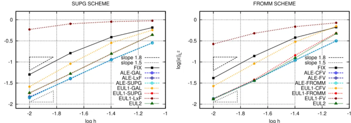
We perform a grid convergence study, and investigate the dependence of the error on the CPU time. We perform the same test for both the RD and FV scheme. In figure 3 the convergence curves for the di↵erent combinations of moving mesh algorithms and interpolations schemes are reported. The interpolation step necessary to evolve the mesh has a positive impact on mesh delay, however the specific scheme used, weakly influences mesh configuration. For the ALE and EUL2 algorithms, we see that all the curves in blue color are almost overlapped. Using this result, in the following numerical test cases, the EUL2 and ALE algorithms will be used in their faster versions with inaccurate interpolation into the MMPDE. On the contrary for the EUL1 algorithm there is only one interpolation scheme which guarentees stable and second order accurate results, actually the one which we evolve the PDE with.
In figure 4 the performances of the di↵erent algorithms are compared in terms of error/time. With the RD method, the ALE algorithm shows the lowest CPU time, for a fixed level of error (roughly 80% faster then a fixed grid computation). The Eulerian algorithms are less efficient because the full two stage RK interpolation had to be implemented (60% gain for EUL2 and 35% for EUL1). For the FV scheme the efficiency between ALE and Eulerian algorithms is more similar (ALE and EUL2 80%, EUL1 70%) because this time, in the interpolation step, the second stage of RK seemed to be not necessary, as emerges also from the work of [17]. Finally, for both RD and FV, the EUL2 rapresents a slight improvement respect to the EUL1 algorithm.
0.8 0.85 0.9 0.95 1 1.05 1.1 1.15 0 0.2 0.4 0.6 0.8 1 1.2 1.4 1.6 1.8 2 η y ALE NO WB ALE WB exact sol. -4 -3.5 -3 -2.5 -2 -2.2 -2 -1.8 -1.6 -1.4 log|| ε|| L 2 log h ALE WB ALE NO WB slope 1.8
Figure 2: Linear Advection. Left: Lake at rest for the NO WB ALE formulation and failing in verifiyng Well Balanced. Middle: comparison beteween the numerical solution and exact one on the simmetry line x = 0.5. Right: convergence order for the L2-norm of the error.
-2 -1.5 -1 -0.5 0 -2 -1.8 -1.6 -1.4 -1.2 -1 log|| ε|| L 2 log h SUPG SCHEME slope 1.8 slope 1.5 FIX ALE-GAL ALE-LxF ALE-SUPG EUL1-GAL EUL1-SUPG EUL1-LxF EUL2 -2 -1.5 -1 -0.5 0 -2 -1.8 -1.6 -1.4 -1.2 -1 log|| ε|| L 2 log h FROMM SCHEME slope 1.8 slope 1.5 FIX ALE-CFV ALE-FV ALE-FROMM EUL1-CFV EUL1-FROMM EUL1-FV EUL2
Figure 3: Rotation. Order of convergence: Left, RD scheme. Right, FV scheme.
-2 -1.5 -1 -0.5 0 1 1.5 2 2.5 3 3.5 4 4.5 5 log|| ε|| L 2 log t SUPG SCHEME FIX ALE-GAL ALE-LxF ALE-SUPG EUL1-GAL EUL1-SUPG EUL1-LxF EUL2 -2 -1.5 -1 -0.5 0 1 1.5 2 2.5 3 3.5 4 4.5 5 log|| ε|| L 2 log t FROMM SCHEME FIX ALE-CFV ALE-FV ALE-FROMM EUL1-CFV EUL1-FROMM EUL1-FV EUL2
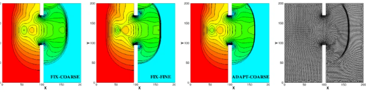
Figure 5: Asymmetric dam-break computed with RD scheme. 30 equispaced contour lines for h and adapted mesh.
Figure 6: Asymmetric dam-break computed with FV scheme. 30 equispaced contour lines for h and adapted mesh.
8
Numerical results for Shallow Water equations
8.1
Asymmetric dam Break
This classical test benchmark, taken from [48], is used to test the adaptive algorithm when bores develop. The set-up consists in a square domain [0⇥ 200]2m with a dam, placed at x = 95 m, separating an upper
and a lower bassin which contain water at di↵erent levels, respectively at 10 m and 5 m. The sudden break of the dam leads to a depression wave advancing in the upper bassin and a bore advancing in the lower bassin. Two corners depression interact, forming a deep trough at the inlet of the dam.
The test is run with both the FV and RD scheme, on a coarse triangulation containing 14538 triangles and 7480 nodes, on a fine one, containing 77302 triangles and 39130 nodes, and on the coarse mesh with adaptive mesh deformation. The typical qualitative result obtained is provided in figures 5 and 6. The pictures show the potential of this adaptation procedure to provide with considerably fewer unknowns a much better resolution of both the smooth and the non-smooth flow features.
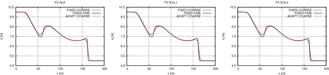
In figures 7,8 a comparison between the ALE algorithm and the EUL1 and EUL2 is shown. For both RD and FV, the ALE algorithm shows a well resolved bore and a correct computation of the trough with a significant saving in CPU time. As shown on table 1, the savings obtained with the ALE algorithm go up to 60% for RD, and 50% for FV. For the RD scheme, the cost of of a two-step interpolation, makes the EUL1 algorithm inefficient, thus the EUL2 a clear improvement. For FV both the interpolation based algorithms (EUL1 and EUL2) are not able of of providing a considerable improvement in the resolution of the peaks and the trough upstream the dam (xw 60), probably due to execessive numerical di↵usion in the interpolation. Some improvement is instead observed with the ALE algorithm, which also gives a much sharper capturing of the bore.
4.5 5.5 6.5 7.5 8.5 9.5 10.5 0 50 100 150 200 η [m] x [m] RD-ALE FIXED-COARSE FIXED-FINE ADAPT-COARSE 4.5 5.5 6.5 7.5 8.5 9.5 10.5 0 50 100 150 200 η [m] x [m] RD-EUL1 FIXED-COARSE FIXED-FINE ADAPT-COARSE 4.5 5.5 6.5 7.5 8.5 9.5 10.5 0 50 100 150 200 η [m] x [m] RD-EUL2 FIXED-COARSE FIXED-FINE ADAPT-COARSE
Figure 7: Asymmetric dam-break computed with RD scheme. Solution along the straight line at y = 132.5 for the di↵erent coupling. Left: ALE. Middle: EUL1. Right EUL2.
4.5 5.5 6.5 7.5 8.5 9.5 10.5 0 50 100 150 200 η [m] x [m] FV-ALE FIXED-COARSE FIXED-FINE ADAPT-COARSE 4.5 5.5 6.5 7.5 8.5 9.5 10.5 0 50 100 150 200 η [m] x [m] FV-EUL1 FIXED-COARSE FIXED-FINE ADAPT-COARSE 4.5 5.5 6.5 7.5 8.5 9.5 10.5 0 50 100 150 200 η [m] x [m] FV-EUL2 FIXED-COARSE FIXED-FINE ADAPT-COARSE
Figure 8: Asymmetric dam-break computed with FV scheme. Solution along the straight line at y = 132.5 for the di↵erent coupling. Left: ALE. Middle: EUL1. Right EUL2.
ALG. MESH (Nodes) RD [s] FV [s]
FIX-COARSE 7480 11.34 11.97
FIX-FINE 39130 185.00 207.14
ADAPT-ALE 7480 77.48 100.16
ADAPT-EUL1 7480 169.63 150.52
ADAPT-EUL2 7480 98.30 111.15
-6e-05 -5e-05 -4e-05 -3e-05 -2e-05 -1e-05 0 1e-05 2e-05 3e-05 4e-05 0 10 20 30 40 50 60 70 80 90 100 Emass t [s]
dambreak with circular hump: RD
r=1 r=2 r=3 -6e-05 -5e-05 -4e-05 -3e-05 -2e-05 -1e-05 0 1e-05 2e-05 3e-05 4e-05 0 10 20 30 40 50 60 70 80 90 100 Emass t [s]
dambreak with circular hump: FV
r=0 r=1 r=2
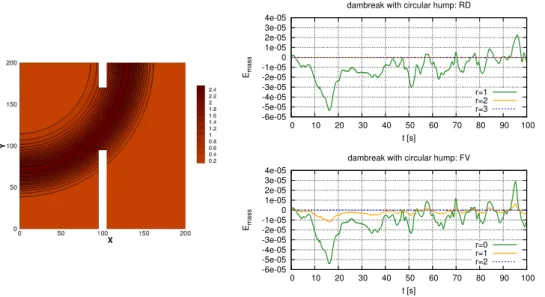
Figure 9: Dambreak with circular hump. Left: bathymetry. Right: dimensionless mass error for di↵erent quadrature formula of the bathymetry integral.
To check our mass conservation correction (cf. section§ 3.3.1) we repeat this test adding a bathymetry shaped as a circular hump centered in (x, y) = (0, 200), and defined by an exponential law in the radial direction (cf. left picture on figure 9). We report on the right pictures on figure 9 the mass error measured without any correction, and with corrections based on di↵erent quadrature formulas (for the definition of Emass, see section§ 3.3.1). We can clearly see that, even for this non-smooth case, we are able to preserve
the total mass in the domain practically up to machine accuracy.
8.2
Small perturbation of a lake at rest
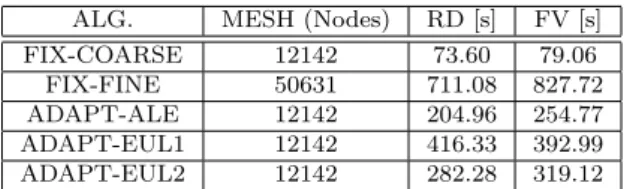
We consider the classical test of a small perturbation over an elliptic exponential hump (se e.g. [48, 14] for details concerning the test setup). This test allows to check the ability of the algorithms proposed to catch relatively smooth wave patterns, and to conserve mass, and the lake at rest state in the unperturbed regions. To run the test, we use a coarse triangulation, containing 12142 nodes and 23852 triangles, and we compute “reference” solutions on a finer mesh, containing 50631 nodes and 100376 triangles.
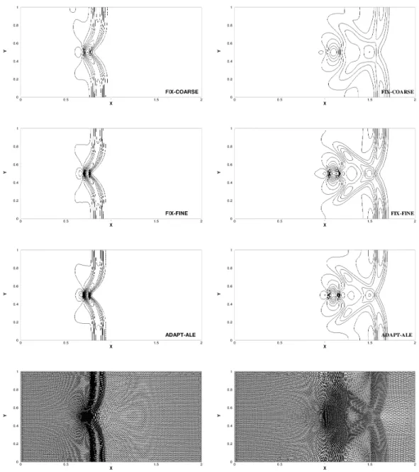
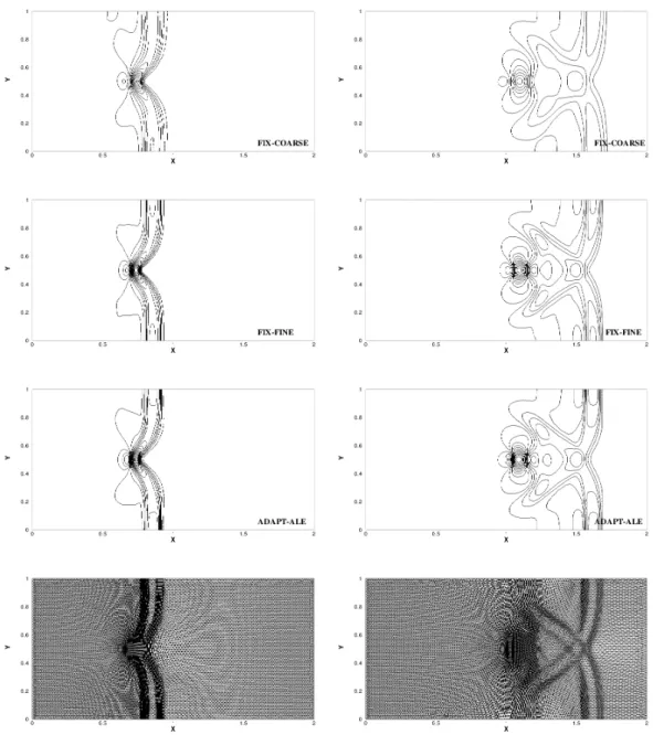
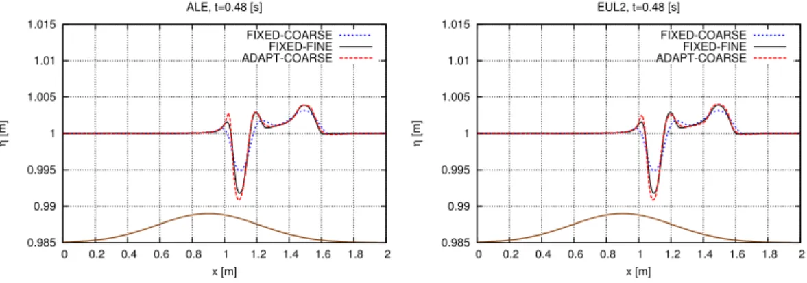
The qualitative behavior of the methods proposed can be seen in figures 10 and 11 (same contour lines drawn in all the pictures). We can see that the mesh follows quite well the propagation and transformation of the waves, providing, on the coarse mesh, a resolution very close to the reference one. No numerical artifacts are observed in the unperturbed region, as a consequence of the exact preservation of the lake at rest state. To perform a more quantitative analysis we report in table 2 the CPU times of all the schemes, and the water height along the line at y=0.5 on figures 12 and 13. For clarity, only the EUL2 method results are plotted in the latter figures, the EUL1 algorithm providing virtually identical solutions. The cuts show how both the ALE and the rezoning algorithms provide solutions close to the reference one. The CPU time savings w.r.t. the reference are of the order of 70% for the ALE method, of 60% for the EUL2, and between 50% (for FV) and 40% (for RD) for the EUL1 algorithm.
Finally, figure 14 shows a study of mass conservation, providing additional proof that the corrections proposed allows to retain the physical mass in the domain virtually to machine accuracy.
Figure 10: Small perturbation of a lake at rest (RD scheme). Solution isolines at t = 0.24, t = 0.48 are shown for fixed grid and adaptive computations. Top: fixed coarse grid. Middle: fixed fine grid. Bottom: adaptive ALE scheme.