A mechanistic model to predict distribution of carbon among multiple sinks.

A mechanistic model to predict distribution of carbon among multiple

sinks.

3

André Lacointe(1), Peter E.H. Minchin(2) 4

5

(1) Université Clermont Auvergne, INRA, PIAF, F-63000, Clermont-Ferrand, France; email: 6

andre.lacointe@inra.fr 7

8

(2) New Zealand Institute for Plant and Food Research, Motueka Research Centre, Motueka, 9

New Zealand; email: Peter.Minchin@plantandfood.co.nz 10

11 12

Abstract/summary.

13

Modelling is a fundamental part of quantitative science. It is a methodology of the holistic 14

approach of bringing together quantitative ideas, many of which will have been developed 15

though a reductionist approach that allows a lot of detail to be gathered on a small part of the 16

system of interest. Phloem and xylem physiology are both descriptions of whole plant 17

behaviour. The phloem is especially difficult to study in a reductionist way because as soon as 18

the phloem is disturbed, even very carefully, it stops functioning by induction of blockage and 19

other defensive mechanisms. This was the cause of a long debate on the basic structure of the 20

phloem’s long-distance transport pathway. Were the sieve-tubes ‘blocked’ at the sieve-plates 21

or was there a continuous open conduit between source and sink? Developments in very rapid 22

chilling of small pieces of phloem tissue, to obtain the required speed of cooling, was needed 23

before reliable micrographs could be obtained and conclusively showed that the observed 24

sieve-plate blockages were an artefact brought about by phloem damage quickly leading to 25

blockage mechanisms, believed to be needed to prevent loss of significant phloem sap when 26

plants are damaged 27

It is now generally accepted that phloem flow is the result of bulk solution flow generated by 28

osmotic pressure generated by phloem loading. But there is still little agreement on how sink 29

competition functions and the well documented source sink relations observed with tracer 30

studies. More recently the importance of phloem pathway leakage (unloading) and reloading 31

has been recognised and the role of this is still being unravelled. Interactions between phloem 1

and xylem flows are now thought to be important, and may have a role in carbohydrate 2

source-sink relations through potassium recirculation. 3

All of these areas are extremely difficult to research by the reductionist approach, with 4

modelling being an important tool to test the consequences of proposed mechanisms which 5

can then be tested in whole plant experiments. 6

Phloem/xylem modelling has been at the limits of quantitative modelling, especially when 7

dynamic models are needed to explain tracer studies. Huge advances in computing now 8

enable more realistic modelling and the PiafMunch approach has extended that even further 9

by enabling much more mechanistic detail to be incorporated. With the recent introduction of 10

tracer dynamics now incorporated in PiafMunch it will be possible to look at the effects of 11

specific phloem mechanisms upon the shape of evolving tracer profiles. 12

13 14

Keywords: Münch model, carbon allocation, sink priority, phloem, xylem, coupled water and

15

carbon fluxes, plant architecture, functional - structural plant modelling, source sink relations 16

1

Introduction

2

Wardlaw (1990) reviewed a large body of experimental data on carbon partitioning in plants 3

and found no mechanistic understanding of the data. More recently Lacointe (2000) reviewed 4

the range of models used in functional-structural tree models where he reviewed the empirical 5

methods based on allometery, sink priorities and functional equilibrium, but found no 6

mechanistic approaches to this fundamental aspect of balanced plant growth. 7

8

Currently, the general consensus of phloem flow is that proposed by Münch (1928) with bulk 9

flow of phloem sap driven by an osmotically generated pressure gradient created by loading 10

of photosynthate (usually sucrose) at the source and unloading at the sink. In many plant 11

species phloem loading is an active transport process across the sieve-tube plasmalemma 12

resulting in a source solute concentration in the order of 0.8 M while in other species this is a 13

passive process relying on diffusional flow from the cells associated with photosynthesis. 14

Detailed biophysical models of this process were first described by Christy and Ferrier (1973) 15

and this work has had considerable complexity added resulting in the recent work of 16

Thompson and Holbrook (2003). This work describes a single-source single-sink system with 17

concomitant water flow in terms of parameters describing phloem loading, phloem unloading, 18

and includes lateral water flow through an ideal (i.e. reflection coefficient for the solute is 19

one) sieve-tube plasmalemma. 20

21

The first attempt to extend this approach to multiple sinks supplied by a single source was that 22

of Minchin et al. (1993). Their simple 2-sink model was able to mimic several observed 23

phenomena involving shoot-root interactions and gave the first quantitative explanation of 24

sink priority. This model predicted that the relative sink priorities between the shoot and root 25

of a barley seedling could be reversed by cooling the root, and this was subsequently 1

demonstrated (Minchin et al., 1994). This preliminary model was based on a non-permeable, 2

either by water or solute, long-distance transport pathway which is known not to be the case. 3

This simplification greatly simplified the model equations allowing them to be solved 4

analytically. Bidel et al. (2000) expanded this approach to many sinks representing a growing 5

root and used an iterative approach to determine how carbohydrate flows were able to mimic 6

different patterns of root growth by altering the individual sink properties. 7

8

But it is well know that the plant vasculature consists of both phloem and xylem which are 9

physically close and readily interact through both water relations and controlled transfer of 10

solutes. Daudet et al. (2002) incorporated xylem/phloem interactions through water relations 11

which could now incorporate effects of transpiration-induced gradients of water potential. 12

Local gradients of all water- and carbon-flux related variables could be accounted for by a 13

spatially discretized approach, which turned partial differential to ordinary differential 14

equations. They used P-SpiceTM software to illustrate their methods on a branching system 15

with three source leaves, and three competing fruits. This work has been extended (Lacointe 16

and Minchin, 2008) to allow huge flexibility in architecture and specific mechanistic detail 17

through use of recently developed numerical methods, resulting in the model ‘PiafMunch’. 18

Recently, Hall and Minchin (2013) proposed a closed-form solution for steady-state coupled 19

phloem/xylem using the Lambert-W function, which can handle multiple sinks. While 20

incorporating some of the added complexities, such as variation of phloem resistance with 21

solute concentration, and deviations in the Van’t Hoff expression for osmotic pressure, the 22

differential equation approach is still quite limited in its ability to handle a lot of detail of 23

physiological interest (e.g. pathway unloading/reloading of solute, different unloading 24

kinetics). By contrast, a major advantage of the PiafMunch approach is its flexibility to be 1

able to work with a huge range of local loading and unloading mechanisms. 2

3

In this chapter, we will first describe the original PiafMunch model as published in 2008 in 4

detail. Then its capacities will be illustrated by examples of use and results. The third part will 5

introduce recent and current developments regarding (i) a more general description of the 6

plant architecture, and (ii) inclusion of additional, refined biophysical or metabolic processes. 7

Finally, practical details will be given to help potential users to handle the model efficiently. 8

9

PiafMunch -- the original model (Lacointe and Minchin, 2008)

10

As a functional-structural model, PiafMunch includes both an architectural description of the 11

plant structure and a mechanistic description of relevant biophysical processes at local level. 12

13

Discretisation of the plant structure

14

The plant skeleton is discretized into an arbitrary number of segments delimited by junction 15

nodes1 (Fig. 1). The plant architecture is thus represented as a collection of elements, each 16

consisting of a topological node and an associated axial pathway segment, with the exception 17

of the ‘collar’ node, whose physical connecting upward and downward pathway segments are 18

conventionally assigned respectively to its upper stem and lower root elements. Most 19

elements are connected to one upper and one lower element, except for the ends of roots 20

where there is no ‘lower’ element, the ends of stems where there is no 'upper' element, and 21

branching elements which have a single connection at one end and two at the other. Thus, a 22

total of seven different element types (denoted by different colours in Fig. 1) are required and 23

sufficient to describe any branched architecture. 24

1

the term ‘node’ here is being used in the topological sense, without reference to botanical nodes which bear the leaves on a plant shoot. In future we will simply use the term node.

1

Local hydraulic architecture

2

Each axial pathway segment includes one phloem and one xylem pathway, which are 3

connected to each other by a transverse pathway (Fig.2) allowing for lateral water exchanges 4

between the sieve tube and local apoplasm. At end nodes, water exchanges with external 5

environment are represented, either as imposed local fluxes (e.g. measured transpiration 6

rates), or constrained by outside (e.g. soil) local water potential. Those represent the system 7

boundary conditions, which are allowed to fluctuate. 8

9

Hydraulic fluxes

10

According to the accepted Münch theory (1928), viscous flow of phloem sap is driven by an 11

axial hydraulic pressure gradient generated by active loading of solutes at the source and 12

unloading in the sink. Lateral solute leakage with reloading occurs along the long-distance 13

pathway, as does lateral water flow determined by water potential gradients and sieve-tube 14

membrane water permeability. 15

Xylem flow is driven by the axial apoplastic pressure gradient generated by leaf 16

transpiration. 17

These basic principles are expressed for each element as a set of equations involving 18

its own local variables and parameters. The volume fluxes of xylem and phloem water are 19

respectively 20

= ∆ / xylem flow between connected elements (1) 21

= ∆ / phloem flow between connected elements (2) 22

The phloem sieve tube resistance rST can be either entered as a local parameter or estimated

23

from sieve tube geometry and sap viscosity (Thompson and Holbrook 2003 – see chapters 22 24

and 26 in this book). Sap viscosity is dependent on temperature and solute concentration, 25

which is empirically described by an exponential to within 1% of experimental values over a 1

wide range of temperatures and concentrations (Gilli 1997, after Mathlouthi and Génotelle 2

1995). 3

Lateral water flow from xylem to phloem sieve tube is driven by the difference in 4

water potential: 5

= ( − )/ (3)

6

where rlat is the sum of the apoplastic pathway resistance between xylem and phloem and the

7

sieve-tube cross-membrane resistance, which is inversely proportional to the membrane 8

permeability. 9

Taking into account the non-zero partial molal volume of sucrose V adds an extra 10

lateral component NZS to the volume flow into the sieve tubes: 11

= + ( − )/ (3’)

12

NZS = ∙ (3”)

13

where JSlat is the lateral solute flow (see next section).

14

Hydrostatic pressure PST within the sieve tubes is given by the difference between total

15

phloem water potential and osmotic potential inside sieve tubes: 16

PST =ΨST -

Π

17

Xylem sap has a very low solute concentration which we shall ignore, so there is no osmotic 18

component to its total water potential: 19

PXyl = ΨXyl (4’)

20

For a single phloem solute,

Π

21

Π

22

ΠST = -R T CST (5)

where R is the universal gas constant and T the absolute temperature. For a non-dilute 1

solution we use the empirical equation stated by Thompson and Holbrook (2003): 2

ΠST = -ρw R T (0.998 m + 0.089 m²) (5’)

3

with

ρ

= / (1 − ∙ ) (5’’)

5

If the partial molal volume of sucrose V is taken as zero then equations 5’ and 5’’ reduces to 6

the Van’t Hoff relation (5), and equation (3’) reduces to the Ohm’s law analog (3). When the 7

solute is sucrose and the concentration is 1 mol L-1 (typical at the site of phloem loading) then 8

using the Van’t Hoff relation for a dilute solution results in about an 8% error in

Π

9

0.5 mol L-1 sucrose this reduces to a 2% error. As this is low enough in most situations 10

(compared to other error sources e.g. in the model parameter values), this refinement can be 11

deactivated by the user to reduce computation time. 12

13

The set of water-flow equations for each element is completed by a flow conservation 14

statement for each of the two hydraulic pathways within an element, one for the xylem and 15

one for the phloem (Fig. 2): 16

17 17 (6)

18

where JW_k (with appropriate sign) represents the lateral and all longitudinal liquid flows

19

to/from the node k, the number of which depends on the element type as defined above. In 20

particular, xylem flow for terminal elements includes transpiration at stem ends (‘leaves’) and 21

water uptake from soil at the root tips (Fig. 2). Note that eq. (6) assumes unchanging sieve 22

tube volume (rigid sieve-tube cell walls), which Thompson and Holbrook (2003) showed to 23

be an acceptable approximation in many situations. 24

25

! _# #

Solute flows

1

Longitudinal phloem solute flow between two connected elements is given by: 2

JSST = JWST· CST (7)

3

where CST is the sieve-tube solute concentration in the upflow element.

4 5

Variation of sieve-tube solute content QST (= CST ∙ VST) is:

6 7

8 8 (8)

where JS_k (with appropriate sign) represents all longitudinal solute flows from/to the

9

connected element(s), and JSlat is the lateral solute flow into the sieve-tube.

10 11

The lateral solute flow rate JSlat , i.e. the local unloading/reloading, can be either set directly

12

as an independent equation or derived from local metabolism (e.g. respiration, photosynthesis 13

or starch ↔ soluble sugar conversion) occurring in an attached parenchyma compartment. 14

This is up to users who can write their own set of equations for JSlat which can have any

15

form, including ordinary differential equations. However, a predefined set of classical 16

equations is proposed for convenience : 17

JSlat = k1·(CPar – CST)·VST + (k2 CPar + k3) VPar (9)

18

where CPar is the parenchyma solute concentration, VST the sieve-tube volume and VPar the

19

parenchyma volume. This allows a number of different dynamics by assigning specific 20

values to local parameters k1, k2, k3, e.g.:

21

- diffusion-like kinetics (k2 = k3 = 0);

22

- constant loading/unloading (k1 = k2 = 0);

23

- concentration-dependent loading with a target concentration Ctarg

24

(k2 = -k1 V /VPar , k3 = k1 Ctarg VST /VPar);

25

%& '

- concentration-dependent unloading as in Thompson and Holbrook (2003) 1

( k3 = 0, k2 = -k1 VST /VPar)

2

such that simple cases of symplastic loading/unloading are currently built into equation (9). 3

The default equation for parenchyma solute content QPar (= CPar ∙ VPar) change rate simulates

4

the result of sucrose exchange with local sieve tubes (JSlat , eq. 9), exchange with

5

environment (maintenance respiration and/or photosynthesis) and starch/sucrose 6

interconversion: 7

8 8 (10)

9

where respiration RM, photosynthesis Ph, and starch S are all expressed in sucrose equivalents.

10

The dynamics of photosynthesis Ph may be either read from an external file or modelled by 11

the user e.g. as a periodic function (Daudet et al., 2002). For maintenance respiration RM , the

12

proposed formalism is that of Thornley (1970; see review by Le Roux et al., 2001), with a 13

concentration-dependent maintenance coefficient to account for phloem sucrose leakage / 14

active reloading: 15

RM = (k4 + k5 CST) Sr (11)

16

where Sr is the structural carbon content of the element biomass, expressed in sucrose 17

equivalents. 18

19

The default representation of starch metabolism uses a general equation derived from Daudet 20 et al. (2002): 21 (12) 22 23

allowing simulation of a number of dynamics, e.g. Michaelis-Menten kinetics for synthesis 24

from a sucrose substrate (through parameters vmax and kM), starch content-dependent

25

dS

dt

%& *

hydrolysis back to sucrose (parameter khyd) or sucrose concentration-dependent

1

interconversion with a target concentration Ctarg.

2 3

All solute-fluxes equations are fully editable, with a possible redefinition of all predefined 4

parameters or definition of new ones, allowing e.g. very simple configurations like Minchin et 5

al. (1993) or Thompson and Holbrook (2003) which were used to test the model (Table 2). If

6

edited, it is up to the user to make sure that the equations make sense. By contrast, all water-7

fluxes equations, which are the heart of the model, are hard coded except for parameters. The 8

full system is coded in C++ and solved by a combination of LAPACK linear algebra package 9

(Anderson et al., 1999) with the sparse extension TAUCS (Toledo, 2003 ) and SUNDIALS 10

algebraic/differential equation solver package (Hindmarsh et al., 2005). The software includes 11

a graphic user interface to specify the architecture, parameters, initial values and other 12

settings. This allows use of the software, with the default equations, without having to 13

recompile it. More flexibility can be achieved be editing the solute fluxes equations and 14

recompiling. 15

16

Examples of what the PiafMunch model has been used on

17

The first application of the PiafMunch software was to a single-source single–sink linked by a 18

5m long distance pathway consisting of a tube of 7.5 µm diameter conduit with membrane 19

permeable to water but not to the solute (sucrose), i.e. a ‘perfect’ semipermeable membrane, 20

with uniform loading along the first 0.5 m and unloading along the last 0.5 m. This example 21

was chosen for direct comparison with the work of Thompson and Holbrook (2003) using a 22

continuous differential equation framework. With the PiafMunch approach we started with 23

N=3160 elements and then looked at the effect of reducing N to a much smaller number. 24

With the large value of N the phloem water flux was very similar to that calculated by the 25

continuum approach of Thompson and Holbrook (2003), with the greatest differences being 1

about 2% when the fluxes were changing at the greatest rate (see Lacointe and Minchin 2008, 2

Fig.3). That low 2% discrepancy can be ascribed to the variation of lumen diameter with 3

pressure, which was included in Thompson and Holbrook (2003) but ignored in PiafMunch. 4

With much lower values of the element number N (e.g. N = 30), the two approaches differed 5

most at the sites of most rapid flux change with differences ca. 10%, and were very close in 6

the regions along the long-distance pathway where the water flux was not rapidly changing. 7

When these comparisons were made 24 hr into the simulation when the flows had reached 8

equilibrium, there was only a small difference between the two approaches, even with N as 9

low as 10, with a maximum deviation below 10%. From this it was concluded that the 10

descrete approach of the PiafMunch model resulted in similar results to the continuous 11

method of Thompson and Holbrook (2003), and that the number of discrete elements required 12

for a good approximation of the continuous system does not need to be very high. 13

14

The variation of sap viscosity with sugar concentration was first introduced by Bancal and 15

Soltani (2002) in a simplified Münch model, assuming uniform concentration along the 16

pathway and ignoring membrane permeability. A few years later, Hölttä et al. (2006) 17

introduced the viscosity change in a more realistic model but ignoring the specific partial 18

molal volume of sugar. In both studies, the authors concluded that high sugar loading rates 19

could block phloem transport due to high sap viscosity. PiafMunch incorporates that variation 20

in sap viscosity with solute concentration as well as the partial molal volume of the solute; 21

these refinements can be set on/off by a simple click, either individually or both together. It 22

was confirmed that both of these had significant effect, both on the equilibrium and non-23

equilibrium flux. Work is needed to determine if these effects have any physiological 24

significance. Hölttä et al. (2006) also showed that transpiration rate can be expected to 25

interact with phloem flow, via water relations described by equation 3 above. This was also 1

demonstrated in the initial PiafMunch work (Lacointe and Minchin 2008, Fig. 8). 2

3

The PiafMunch model is meant to handle more complex source-sink configurations. Working 4

with a considerably simplified model with a solute molal volume of zero, constant sap 5

viscosity with changes in solute content, and a non-permeable long-distance transport conduit, 6

Minchin et al. (1993) developed a Munch model describing flow between 1-source and 2-7

sinks which predicted changes in the proportion of total solute flow delivered to each sink 8

when the source supply changed, which in experimental work has been described in terms of 9

sink priority. This was the first mechanistic description of sink priority. Working with the 10

same source sink configuration, and incorporating non-zero pathway permeability the 11

PaifMunch model showed the similar priority behaviour. The main purpose of this work was 12

to determine if the PiafMunch model gave results consistent with previous work, and it passed 13

this test with flying colours so we can have confidence in this new approach and now 14

investigate examples the previous methods cannot handle. 15

16

Thorpe et al. (2011) went on to model a 2-source 3-sink configuration generated in a heavily 17

pruned dwarf bean plant and test the predictions using 11C tracer. Several observed treatment 18

responses were successfully predicted, but the observations could not be completely explained 19

when the modelled common pathway, comprising the stem, contained just one phloem 20

pathway. Bidirectional flow within the stem was necessary to explain the observed flows. 21

It is now accepted that the long-distance phloem transport pathway is leaky, and also takes up 22

solute from the immediate apoplast. This manifests itself in tracer studies through the 23

observed buffering of phloem flow when the phloem pathway is disturbed or there are sudden 24

changes in source or sink function. The PiafMunch model has been used to determine if this 25

leakage/reloading alters source sink dynamics (Minchin and Lacointe, 2017). This modelling 1

indicated that the phloem flow does not follow Poiseuille dynamics, i.e. the water flux was 2

not proportional to ΔP, due to there always being water flow across the membrane, even 3

without pathway unloading and or reloading of solute. At equilibrium, the presence of 4

unloading altered the solute concentration and hydrostatic pressure profiles. With adequate 5

reloading along the pathway the effects of pathway unloading were completely compensated 6

for, making the equilibrium system look like one with no pathway unloading. Further work is 7

needed here to look at the non-equilibrium flows. To do this even more model parameters are 8

needed, though this might be a means of estimating these parameter values through 9

optimising the parameters to produce behaviour similar to that seen in plant experiments. 10

11

Current developments

12

A new version has been developed (PiafMunch v.2) which features a few major 13

improvements: 14

(1) The extension of the architectural pattern from branched to any network

15

architecture, including loops and nodes of any connectivity order (that was limited to

16

3 in v.1, i.e. each node could be connected to 3 other nodes at most). That significantly 17

extends the scope of the model, to e.g. the looped nervation pattern of an isolated leaf, 18

or non-binary, verticillate branching patterns as exhibited by conifers. 19

(2) A significant refinement of the local tissue model at the node level (Fig. 3 and 4),

20

with explicit apoplasmic, possibly solute-containing, compartments attached to both 21

phloem (in addition to the sieve tube) and lateral parenchyma (in addition to 22

symplasm). In particular, the lateral pathway from xylem vessel to phloem sieve tube 23

(rlat, JWlat in eq. 3) is now explicitly segmented into an apoplasmic pathway (rTrsv,

24

JWTrsv) and the cross-membrane pathway from phloem apoplasm to sieve tube (rPhlMb,

JWPhlMb). Water and solute fluxes between adjacent compartments are described by

1

equations similar to (1-9) above, allowing more realistic simulation of e.g. apoplasmic 2

(un)loading and related cross-membrane processes, or a convective component of 3

symplasmic (un)loading.. Again, all parameters and solute flux equations can be 4

redefined or edited to reduce the extended model to v.1 (Lacointe and Minchin 2008), 5

or the simpler Minchin et al. (1993). 6

(3) User-defined sharp parameter changes can be implemented at specific time points,

7

in addition to continuous parameter changes which were already possible in v.1 (with 8

concentration-dependent phloem viscosity as a built-in example). This allows 9

simulation of e.g. cold blocking / unblocking of the phloem pathway or aquaporin 10

function - related changes in cross-membrane resistances (Steppe et al, 2012). 11

(4) Lateral parenchyma symplasmic volumes are now considered variables that can

12

be driven by differential equations involving any other variables like local pressure, 13

allowing simulation of e.g. reversible, elastic volume changes, i.e. water capacitance, 14

involved in reversible stem diameter changes (Steppe et al., 2012), or plastic, 15

irreversible growth (Lockhart, 1965; Daudet et al., 2002). 16

(5) Tracer analysis facilities have been included as a helper to design and analyse results

17

from tracer experiments like that of Thorpe et al. (2011). They involve equations 18

similar to the solute-related equations with additional terms for radioactive decay, in 19

particular for 11C which has a very short half-life of ca. 20 min. 20

21

Concluding remarks

22

PiafMunch has proved highly efficient and reliable on simple systems -- even though they 23

could be more complex than those modelled by other approaches in literature. However, it is 24

meant to handle truly complex architectures and detailed local processes, using highly 25

efficient, state-of-the-art numerical methods. It can be used to simulate and test effects of any 1

known or hypothetical mechanism, both at the local and at the global, plant-wide scale level. 2

It can be used also to simulate coupled solute/water relations of a single, isolated organ, e.g. 3

an isolated leaf, given appropriate boundary conditions dynamics. Furthermore, it can be 4

easily extended, as shown by the development of v.2. This could be readily further extended 5

to e.g. a vacuolar compartment with specific aquaporins mediating tonoplast resistances; 6

another possible extension, though slightly more difficult to implement, would be to introduce 7

multiple phloem pathways as suggested by results from Thorpe et al (2011). It should be 8

emphasized, however, that any extension involves additional parameters (theoretically N 9

additional values for each additional local parameter, although it is often reasonable to assume 10

a common, single value), which can result in unreasonable, and confusing, complexity. This 11

can be handled by setting unnecessary parameters to zero or infinite values to keep focus on 12

those relevant to the issue of interest. Because of the multiplicity of parameters, it is 13

unrealistic to use the model as a means to optimise parameters to fit experimental data; 14

however, this could be made possible by setting a significant subset of parameters to known, 15

reasonable values and optimising only another, limited, focus subset of parameters. This 16

emphasizes the importance of membrane-focused and other experimental studies at the tissue 17

or cell level to provide such required parameter values. As for all modelling, its use is in 18

testing ideas and never a substitute to experiment. 19

20

Potential users interested in implementing PiafMunch in their work are very welcome to 21

contact the authors. We will be pleased to help, either for specific applications or for practical 22

installation details. 23

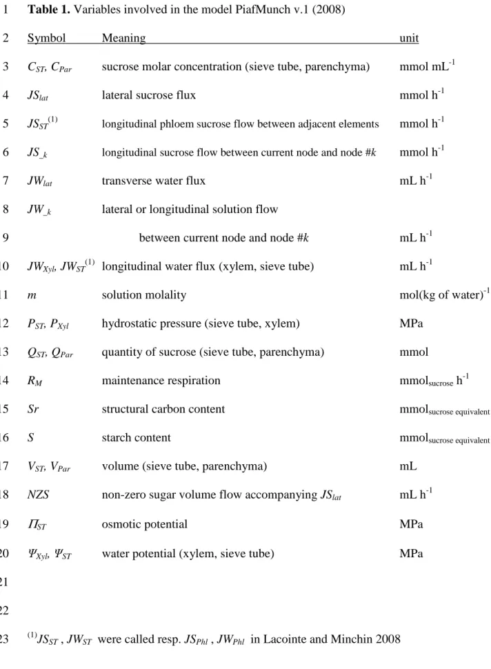
Table 1. Variables involved in the model PiafMunch v.1 (2008)

1

Symbol Meaning unit

2

CST, CPar sucrose molar concentration (sieve tube, parenchyma) mmol mL-1

3

JSlat lateral sucrose flux mmol h-1

4

JSST(1) longitudinal phloem sucrose flow between adjacent elements mmol h-1

5

JS_k longitudinal sucrose flow between current node and node #k mmol h-1

6

JWlat transverse water flux mL h-1

7

JW_k lateral or longitudinal solution flow

8

between current node and node #k mL h-1 9

JWXyl, JWST(1) longitudinal water flux (xylem, sieve tube) mL h-1

10

m solution molality mol(kg of water)-1

11

PST, PXyl hydrostatic pressure (sieve tube, xylem) MPa

12

QST, QPar quantity of sucrose (sieve tube, parenchyma) mmol

13

RM maintenance respiration mmolsucrose h-1

14

Sr structural carbon content mmolsucrose equivalent

15

S starch content mmolsucrose equivalent

16

VST, VPar volume (sieve tube, parenchyma) mL

17

NZS non-zero sugar volume flow accompanying JSlat mL h-1

18

Π

19

ΨXyl, ΨST water potential (xylem, sieve tube) MPa

20 21 22

(1)

JSST , JWST were called resp. JSPhl , JWPhl in Lacointe and Minchin 2008

Table 2. Model parameters 1

Symbol Meaning (equation. involved) value as used to simulate Thompson & Holbrook 2003

Ctarg target sucrose concentration for starch metabolism (eq. 12) 0.1 mmol mL-1 (1) k1

lateral carbon flow rate parameters (eq. 9)

3.23994 h-1 in unloading zone ; 0 elsewhere

k2 -3.23994 h-1 in unloading zone ; 0 elsewhere

k3 0 mmol mL-1 h-1

k4

Maintenance respiration – related parameters (eq. 11)

0 h-1

k5 0 mL mmol-1 h-1

k6 Starch metabolism – related parameter (eq. 12) 0 h-1 khyd relative rate of starch hydrolysis (eq. 12) 0 h-1

kM Michaelis-Menten constant for starch synthesis (eq. 12) 0 mmolsucrose mL-1 (1) Ph rate of photosynthesis (eq. 10) 0 mmolsucrose h-1 (2)

R universal gas constant (eqs. 5, 5’) 0.0083143 MPa mL K-1 mmol-1

rlat lateral hydraulic flow resistance (eq. 3, 3’) 23.5785 x N (3) MPa h mL-1

rST(4) axial phloem sieve tube hydraulic flow resistance (eq. 2) 14050.3 / N (3) MPa h mL-1 for CST = 0.5 mmol mL-1 (4) rXyl axial xylem hydraulic flow resistance (eq. 1) 10-200 / N (3) MPa h mL-1

T absolute temperature (eqs. 5, 5’) 293 K

V partial molal volume of sucrose (eqs. 3’, 5”) 0.2155 mL mmol-1 vmax kinetic parameter for starch synthesis (eq. 12) 0 mmolsucrose equ.mL-1 h-1

w

ρ

software default value, without effect in simulating either Thompson & Holbrook (2003) or Minchin et al (1993). 1

(2)

user-defined input variable (does not have to be constant). 2

(3)

axial (resp. lateral) hydraulic resistances are proportional (resp. inverse proportional) to element length, hence the scaling by N (see text). 3

(4)

rST (called rPhl in Lacointe and Minchin 2008) changes with CST, in proportion to the solution viscosity. 4

1

References

2

Anderson E, Bai Z, Bischof C, Blackford S, Demmel J, et al. (1999). ‘LAPACK users’ guide. 3

3rd edn. http://www.netlib.org/lapack/lug/index.html (accessed 28 March 2018). 4

5

Bancal P, Soltani F (2002). Source-sink partitioning. Do we need Münch? Journal of 6

Experimental Botany 53, 1919-1928.

7 8

Bidel LPR, Pages L, Riviere LM, Pelloux G Lorendeau JY (2000). Mass Flow Dyn 1: A 9

carbon transport and partitioning model for root system architecture. Annals of Botany 10

85, 869-886.

11 12

Christy A.L, Ferrier JM (1973). A mathematical treatment of Munch’s pressure-flow 13

hypothesis of phloem translocation. Plant Physiology 52, 531-538. 14

15

Daudet FA, Lacointe A, Gaudillère JP, Cruiziat P (2002). Generalized Münch coupling 16

between sugar and water fluxes for modelling carbon allocation as affected by water 17

status. Journal of Theoretical Biology 214, 481-498. 18

19

Gilli R (1997). Evaluation de différentes données physico-chimiques relatives aux solutions 20

sucrées. http://www.associationavh.com/fr/feuilles.html (accessed 28 March 2018). 21

22

Hall AJ, Minchin PEH (2013). A closed-form solution for steady-state coupled phloem/xylem 23

flow using the Lambert-W function. Plant, Cell and Environment 36, 2150-2162. 24

Hindmarsh AC, Brown PN, Grant KE, Lee SL, Serban R, Shumaker DE, Woodward CS 1

(2005). SUNDIALS: Suite of Nonlinear and Differential/Algebraic Equation Solvers. 2

ACM Transactions on Mathematical Software 31, 363-396.

3 4

Hölltä T, Vesala T, Sevanto S, Perämäki M, Nikinmaa E (2006). Modeling xylem and phloem 5

water flows in trees according to cohesion theory and Münch hypothesis. Trees 20, 6

67-78. 7

8

Lacointe A (2000). Carbon allocation amoung tree organs. A review of basic processes and 9

representation in functional tree-models. Annals of Forest Science 57, 521-533. 10

11

Lacointe A, Minchin PEH (2008). Modelling phloem and xylem transport within a complex 12

architecture. Functional Plant Biology 35, 772-780. https://doi.org/10.1071/FP08085 13

14

Le Roux X, Lacointe A, Escobar-Gutiérrez A, Le Dizès S (2001). Carbon-based models of 15

individual tree growth: a critical appraisal. Annals of Forest Science 58, 469-506. 16

17

Mathlouthi M, Génotelle J (1995). Rheological properties of sucrose solutions and 18

suspensions. In: ‘Sucrose. Properties and Applications’. (Ed. M.Mathlouthi and P. 19

Reiser) pp. 126-154. (Blackie Academic & Professional) 20

21

Minchin PEH, Thorpe MR, Farrar JF (1993). A simple mechanistic model of phloem 22

transport which explains sink priority. Journal of Experimental Botany 44, 947-955. 23

Minchin PEH, Farrar JF, Thorpe MR (1994). Partitioning of carbon in split roots of barley: 1

effect of temperature of the root. Journal of Experimental Botany 45, 1103-1109. 2

3

Minchin PEH, Lacointe A (2017). Consequences of phloem pathway unloading/reloading on 4

equilibrium flows between source and sink: a modelling approach. Functional Plant 5

Biology 44, 507-514.

6 7

Münch E (1928). Versuche über den Saftkreislauf. Deutsche botanische Gesellschaft 45, 340-8

356. 9

10

Steppe K, Cochard H, Lacointe A, Ameglio T (2012). Could rapid diameter changes be 11

facilitated by a variable hydraulic conductance? Plant, Cell and Environment, 35 (1), 12

150-157. 13

14

Thompson MV, Holbrook NM (2003). Application of a single-solute non-steady-state phloem 15

model to the study of long-distance assimilate transport. Journal of Theoretical 16

Biology 220, 419-455.

17 18

Thornley JMH (1970). Respiration, growth and maintenance in plants. Nature 227, 304–305. 19

20

Thorpe MR, Lacointe A, Minchin PEH (2011).Modelling phloem transport with a pruned 21

dwarf bean: a 2-source- 3-sink system. Functional Plant Biology 38, 127-138. 22

23

Toledo S (2003). TAUCS, a library of sparse linear solvers. 24

http://www.tau.ac.il/~stoledo/taucs (accessed on 28 March 2018)

1

Wardlaw IF (1990). The control of carbon partitioning in plants. New Phytologist 116, 341-2

381. 3

Figure captions

1 2

Figure 1. Representation of plant architecture. In this example, a plant (A) with 2 roots and 3 3

branches each terminated by a leaf, is represented by 18 elements (B) : one collar element 4

(blue, No. 1), six non-branched stem elements (brown; No. 2, 3, 4, 5, 6, 7), three shoot 5

terminations (green; No. 8, 9, 10), two branched stem elements (orange; No. 11, 12), 1 6

branched root element (black; No. 13), three non-branched root elements (dark grey; No. 14, 7

15, 16) and two root tips (light grey; No. 17, 18). Reproduced from Lacointe et al. (2008) 8

with permission from CSIRO Publishing. 9

10

Figure 2. Network of hydraulic pathways for the example presented in Fig.1. The colour 11

coding is the same as in Fig. 1. Reproduced from Lacointe et al. (2008) with permission from 12

CSIRO Publishing. 13

14

Figure 3. The PiafMunch v.2. extended volume flow model. r…, JW…, P…, Ψ…, Π…, V…: resp.,

15

hydraulic resistance, volume flux, turgor pressure, water potential, osmotic potential, volume; 16

for resp. (subscripts): ST, Xyl, Trsv, Apo, PhlMb, ParMb, ParApo, Sympl : sieve tube, xylem, transverse

17

(xylem to phloem) apoplasm, pathway, phloem to lateral parenchyma apoplasm, pathway, 18

sieve tube plamalemma, lateral parenchyma plasmalemma, lateral parenchyma apoplasm, 19

lateral parenchyma symplasm, NZS, NZSPar: non-zero sugar volume flow, resp. into sieve tube

20

and parenchyma symplasm. Operator Δ means ‘[in] – [out]’ when applied to node-to-node-21

connector variables (JWST, JWXyl), or ‘[upflow] – [downflow]’ when applied to node variables

22

(PST, PXyl).

23 24

Figure 4. The PiafMunch v.2. extended solute flow model. JS…, Q…, C …, V…: resp., solute

flux, total solute content, solute concentration, volume; for resp. (subscripts): ST, Apo,PhlMb,

1

ParMb, ParApo, Sympl : sieve tube, phloem to lateral parenchyma apoplasm, pathway, sieve tube

2

plamalemma, lateral parenchyma plasmalemma, lateral parenchyma apoplasm, lateral 3

parenchyma symplasm. Operator Δ means ‘[in] – [out]’. 4

Figure 1 1 2 3 A B 4 5 1 2 5 10 6 14 3 7 9 4 8 18 16 15 17 13 12 11

Figure 2. 1 1 2 5 10 6 14 3 7 9 4 8 18 16 15 17 13 12 11 collar ► Hydraulic architecture : hydraulic node phloem pathway transverse pathway xylem pathway leaf transpiration water uptake from soil

Phloem

sieve tube

Xylem

vessel

Lateral tissues

►

►

►

►

JW

JW

.in

JW

.out,

Transpirat.

JW

.in,

Root Absorb.

(P=Ψ)

(P,Ψ)

●

●

►

●

(P,Ψ)

(P,Ψ)

●

●

(P,Ψ)

►

►

JW

JW

.out

P_Xyl- P_PhlApo= r_Trsv· JW_Trsv

Ψ_ST = P_ST + Π_ST

Ψ_PhlApo– Ψ_ST = r_PhlMb· JW_PhlMb

dV_Sympl/dt = JW_ParMb- JW_Sympl+ NZS_Par

P_Sympl– P_ST = r_Sympl· JW_Sympl

P_PhlApo- P_ParApo= r_Apo· JW_Apo

JW_Apo= JW_ParMb

Ψ_ParApo- Ψ_Sympl= r_ParMb· JW_ParMb

JW_Trsv= JW_PhlMb+ JW_Apo

Ψ_Sympl= P_Sympl+ Π_Sympl

Ψ_ParApo= P_ParApo+ Π_ParApo

Ψ_PhlApo= P_PhlApo+ Π_PhlApo

ΔJW_ST = -NZS - JW_PhlMb- JW_Sympl

Figure 3 1

Biological membrane Non-membr. boundary

►

JS

.in

JS

JS

.out

Q

Phloem

sieve tube

►

►

Q

Q

Q

►

JS

Lateral tissues

dQSympl/ dt = JSParMb- JSSympl+ (user-defined)

JS_Sympl= C_sympl|ST· JW_Sympl

CSympl= QSympl/ VSympl

JSParMb= (user-defined)

dQPhlApo/ dt = - JSPhlMb - JSApo+ (user-defined)

dQParApo/ dt = JSApo– JSParMb+ (user-defined)

JSApo= (user-defined)

CParApo= QParApo/ VParApo

C_PhlApo= Q_PhlApo/ V_PhlApo

Figure 4 1