HAL Id: halshs-00788647
https://halshs.archives-ouvertes.fr/halshs-00788647
Submitted on 14 Feb 2013
HAL is a multi-disciplinary open access
archive for the deposit and dissemination of sci-entific research documents, whether they are pub-lished or not. The documents may come from teaching and research institutions in France or abroad, or from public or private research centers.
L’archive ouverte pluridisciplinaire HAL, est destinée au dépôt et à la diffusion de documents scientifiques de niveau recherche, publiés ou non, émanant des établissements d’enseignement et de recherche français ou étrangers, des laboratoires publics ou privés.
Aggregating sets of von Neumann-Morgenstern utilities
Eric Danan, Thibault Gajdos, Jean-Marc Tallon
To cite this version:
Eric Danan, Thibault Gajdos, Jean-Marc Tallon. Aggregating sets of von Neumann-Morgenstern utilities. Journal of Economic Theory, Elsevier, 2013, 148 (2), pp.663-688. �10.1016/j.jet.2012.12.018�. �halshs-00788647�
Aggregating sets of von Neumann-Morgenstern
utilities
∗
Eric Danan
†Thibault Gajdos
‡Jean-Marc Tallon
§July 25, 2012
Abstract
We analyze the preference aggregation problem without the assumption that individuals and society have fully determined and observable preferences. More precisely, we endow individuals and society with sets of possible von Neumann-Morgenstern utility functions over lotteries. We generalize the classical Pareto and Independence of Irrelevant Alternatives axioms and show they imply a generaliza-tion of the classical neutrality assumpgeneraliza-tion. We then characterize the class of neutral social welfare functions. This class is considerably broader for indeterminate than for determinate utilities, where it basically reduces to utilitarianism. We finally characterize several classes of neutral social welfare functions for indeterminate utilities, including the utilitarian and “multi-utilitarian” classes.
Keywords. Aggregation, vNM utility, indeterminacy, neutrality, utilitarianism. JEL Classification. D71, D81.
1
Introduction
A common feature of social choice theory is the assumption that individual have com-pletely determined preferences or utilities, that are fully identified by the social planner. Such an assumption might, however, seem very demanding. First, individuals may en-vision more than one utility function, either because their preferences are incomplete
∗We thank Philippe Mongin, three referees, and an associate editor for useful comments and
discus-sions, as well as audience at London School of Economics, Universit´e Paris Descartes, ´Ecole Polytech-nique, and D-TEA 2010. Financial support from ANR ComSoc (ANR-09-BLAN-0305-03) is gratefully acknowledged.
†Universit´e de Cergy-Pontoise, THEMA, 33 boulevard du Port, 95000 Cergy-Pontoise cedex, France.
E-mail: Eric.Danan@u-cergy.fr.
‡Aix-Marseille University (Aix-Marseille School of Economics), CNRS, and EHESS. E-mail:
thibault.gajdos@univmed.fr
§Paris School of Economics, Universit´e Paris I Panth´eon-Sobronne, CNRS. E-mail:
(Aumann [2], Bewley [3], Dubra et al. [11], Evren and Ok [12]), or because they are uncertain about their tastes (Cerreia-Vioglio [5], Dekel et al. [10], Koopmans [15], Kreps [16]), or because they are driven by several “selves” or “rationales” (Ambrus and Rozen [1], Green and Hojman [13], Kalai et al. [14], May [17]). Second, even if all individuals have single, fully determined utility functions, fully identifying them may be either in-feasible or too costly, so that the social planner may be unable or unwilling to assign a precise utility function to each individual (C.Manski [6, 7]).
This paper proposes a first step towards a social choice theory allowing for situations in which individuals have only partially determined preferences or utilities. In order to account for such situations, we endow individuals with sets of utility functions. Such a set represents the possible utility functions the individual may have, according to the social planner. The particular case where this set is a singleton then corresponds to the standard setting in which the individual has a single, fully determined utility function. We shall say that the utility function is determinate in this case and indeterminate otherwise, to summarize the different situations mentioned above.
We consider risky alternatives and study social welfare functions mapping profiles of individual von Neumann-Morgenstern (henceforth vNM) utility sets to social vNM utility sets. In this setting, when utility functions are determinate, classical Pareto and Independence of Irrelevant Alternatives axioms lead to a very specific and tractable form of the social welfare function: utilitarianism (Coulhon and Mongin [8]). Specifically, the Pareto and Independence of Irrelevant Alternatives axioms together yield a classical neutrality property: the social utility level is a function of the individual utility levels only. Linearity of the vNM utility function then straightforwardly implies linearity of the social utility level in the individual utility levels. Hence, the social utility function is a linear combination of the individual utility functions.
As it turns out, moving from determinate to indeterminate utilities makes things much more complex even in this simple setting. First, in general, there is not a single utility level, but a set (in fact, an interval) of possible utility levels for each alterna-tive, so that the classical neutrality property cannot be used. Natural generalizations of the Pareto and Independence of Irrelevant Alternatives axioms nevertheless yield a generalized “interval-neutrality” property: the social utility interval is a function of the individual utility intervals only. Second, linearity of vNM utility functions does not imply any linearity property for utility intervals. It however yields weaker convexity properties which, together with other regularity properties, allow us to express the social utility interval as a union of linear combinations of individual utility intervals. Third, pinning down the utility intervals for all alternatives is not enough to fully pin down the social utility set. Despite this, the generalized axioms are powerful enough to yield full-fledged characterization results.
the generalized Pareto and Independence of Irrelevant Alternatives axioms. In Section 3 the interval-neutrality property is defined and shown to be implied by the Pareto and Independence of Irrelevant Alternatives axioms, and a characterization of interval-neutral social welfare functions is provided. This characterization of interval neutrality, although falling short of fully pinning down the social utility set, is the key technical step towards full-fledged characterization results, which are obtained in Section 4. In particular, the classes of utilitarian and “multi-utilitarian” social welfare functions are characterized, and their degree of “social indeterminacy” is analyzed. Section 5 provides generalizations of the preceding results to more general alternatives and domains. Section 6 concludes. Proofs are gathered in the Appendix.
2
Setup
Let X be a non-empty set of social alternatives. We assume that X is a set of probability measures (lotteries) over a non-empty set Z of social (sure) outcomes and that, further-more, X is convex and contains all probability measures on Z with finite support (simple lotteries). Thus we may for instance take X to be the set of all probability measures on Z with finite, countable, or (if a topology on Z is given) compact support. We will maintain this assumption on X until Section 5, in which we will consider more general sets of alternatives. Given two alternatives x, y ∈ X and a number λ ∈ [0, 1], we let xλy denote the convex combination λx + (1 − λ)y ∈ X.
A utility function u on X associates to each alternative x ∈ X a utility level u(x) ∈ R. A utility function u on X is a vNM utility function if it is affine, i.e. if u(xλy) = λu(x) + (1 − λ)u(y) for all x, y ∈ X and all λ ∈ [0, 1]. Let P ⊆ RX denote the set of all vNM
utility functions on X. P is a linear subspace of RX and contains all constant functions.
Given a real number γ ∈ R, we abuse notation by also letting γ denote the corresponding constant function in P .
We consider non-empty sets of utility functions, i.e. non-empty subsets of RX. Our
interpretation of such a set is that the utility function may possibly be any member of the set, without further information being available. The utility function is determinate if the set is a singleton and indeterminate otherwise. We restrict attention to sets of vNM utility functions. More precisely, let P denote the set of all non-empty, compact, and convex subsets of P , where P is endowed with the subspace topology and RX with
the product topology. Note that P contains in particular all convex hulls of finite sets of vNM utility functions on X and, hence, all singletons.
A vNM utility set U ∈ P can be seen as representing an underlying preference relation % over alternatives in X, in the sense that for all x, y ∈ X,
The special case where U is a singleton then corresponds to standard expected utility preferences (von Neumann and Morgenstern [19]). When U is not a singleton, on the other hand, the preference relation % is incomplete, i.e. there are alternatives x, y ∈ X such that neither x % y nor y % x (unless all elements of U are positive affine transformations of one another), but satisfies all the other standard vNM axioms. Shapley and Baucells [23] axiomatize the existence of a closed and convex subset U of P satisfying (1), whereas Dubra et al. [11], assuming X is the set of all Borel probability measures on a compact metric space Z, axiomatize the existence of a closed and convex set U of continuous functions in P satisfying (1).1
Let I be a non-empty and finite set of individuals. Given a non-empty domain D ⊆ PI, a social welfare function F on D associates to each profile (U
i)i∈I ∈ D of individual
(vNM) utility sets a social (vNM) utility set U = F ((Ui)i∈I) ∈ P. We will maintain the
assumption that D = PI from now on, and will relax it in Section 5.
The most classical axioms for social welfare functions with determinate utilities are the Pareto and Independence of Irrelevant Alternatives axioms. Both of them can be generalized to indeterminate utilities. The Pareto Indifference (resp. Pareto Weak Pref-erence) axiom requires that if all individuals are indifferent between alternatives x and y (resp. weakly prefer x to y) then so does society. To the extent that a utility set U ∈ P can be seen as representing an underlying preference relation in the sense of (1), it is natural to generalize the Pareto axioms to utility sets as follows.
Axiom 1 (Pareto Indifference). For all (Ui)i∈I ∈ D and all x, y ∈ X, if ui(x) = ui(y) for
all ui ∈ Ui and all i ∈ I then u(x) = u(y) for all u ∈ F ((Ui)i∈I).
Axiom 2(Pareto Weak Preference). For all (Ui)i∈I ∈ D and all x, y ∈ X, if ui(x) ≥ ui(y)
for all ui ∈ Ui and all i ∈ I then u(x) ≥ u(y) for all u ∈ F ((Ui)i∈I).
Independence of Irrelevant Alternatives essentially requires the social ranking between alternatives x and y to depend only on the individual rankings between x and y. Again, to the extent that a utility set U ∈ P can be seen as representing an underlying preference relation in the sense of (1), it is natural to view the ranking between x and y as determined by the set {(u(x), u(y)) : u ∈ U}. Let us introduce the following notation: given a subset Y of X and a utility set U ∈ P, let U|Y denote the restriction of U to Y , i.e.
1Neither of these two results fully characterize the existence of a utility set U ∈ P satisfying (1).
Indeed, the set U in the former result cannot be taken to be compact in general. However, a sufficient condition for the existence of a compact U is that all functions in U be bounded (since we can then scale all these functions down to range within a given bounded interval and then take the closure of the convex hull of these scaled functions), and this sufficient condition will obtain in particular if either Z is finite or X contains all probability measures on Z with countable support. The set U in the latter result, on the other hand, can always be taken to be compact (because all utility functions in this set are necessarily bounded), but the additional continuity property rules out some members of P, unless Z is finite.
U|Y = {u|Y : u ∈ U}.2 We thus generalize the Independence of Irrelevant Alternatives
axiom to utility sets as follows.
Axiom 3 (Independence of Irrelevant Alternatives). For all (Ui)i∈I, (Ui′)i∈I ∈ D and all
x, y ∈ X, if Ui|{x,y} = Ui′|{x,y} for all i ∈ I then F ((Ui)i∈I)|{x,y} = F ((Ui′)i∈I)|{x,y}.
For a social welfare function with determinate utilities, Independence of Irrelevant Alternatives implies that the restriction of the social utility function to any finite subset of alternatives depends only on the restrictions of the individual utility functions to this subset of alternatives (Blau [4], D’Aspremont and Gevers [9]). This is simply because any function is fully determined by its restrictions to all pairs of elements of its domain. This argument does not hold for indeterminate utilities: a set of functions on a common domain is generally not fully determined by the corresponding sets of restrictions to all pairs of elements of the domain, because there is generally more than one way of “gluing” together these sets of restrictions. Nevertheless, because we restrict attention to vNM utility functions, it can in fact be shown that Independence of Irrelevant Alternatives still implies that the restriction of the social utility set to any finite subset of alternatives depends only on the restrictions of the individual utility sets to this subset of alternatives in our setting (see Lemma 15 in the Appendix).
3
Interval neutrality
In the classical Arrovian framework, neutrality refers to the fact that if alternatives x and y are ranked by individuals in a given situation (i.e. for a given profile of individual preferences) exactly as alternatives z and w are in another situation, then the social ranking between x and y in the first situation is the same as the social ranking between z and w in the second one. In the richer framework of social welfare functions with determinate utilities, neutrality means that if the individual utility levels of alternatives x and y in a given situation are the same as the individual utility levels of alternatives z and w in another situation, then the social ranking between x and y in the first situation is the same as the social ranking between z and w in the second one (Sen [22]). If profiles of individual utility functions are mapped to social utility functions rather than social preference relations, then neutrality can be simply stated by requiring that if the individual utility levels of alternative x in a given situation are the same as the individual utility levels of alternative y in another situation, then the social utility level of x in the first situation is the same as the social utility level of y in the second situation (Coulhon and Mongin [8]).
2Given a function f on a set S and a subset T of S, f |
T denotes the function on T defined by
When the utility function is indeterminate, however, an alternative does not in general have a single utility level but rather a set (in fact, a non-empty and compact interval) of possible utility levels. More precisely, given a utility set U ∈ P, let U(x) = U|{x} denote
the utility interval of an alternative x ∈ X. We generalize the neutrality property by requiring that if the individual utility intervals of alternative x in a given situation are the same as the individual utility intervals of alternative y in another situation, then the social utility interval of x in the first situation is the same as the social utility interval of y in the second situation.
Definition 1 (Interval-neutrality). A social welfare function F on a domain D ⊆ PI is
interval-neutral if for all (Ui)i∈I, (Ui′)i∈I ∈ D and all x, y ∈ X, if Ui(x) = Ui′(y) for all
i ∈ I then F ((Ui)i∈I)(x) = F ((Ui′)i∈I)(y).
For determinate utilities, neutrality is equivalent to the conjunction of Independence of Irrelevant Alternatives and Pareto Indifference. This equivalence does not hold in our framework, but, it is still the case that Independence of Irrelevant Alternatives and Pareto Indifference together imply interval-neutrality.
Lemma 1. If a social welfare function F on D = PI satisfies Independence of Irrelevant
Alternatives and Pareto Indifference then F is interval-neutral.
To show that the converse of Lemma 1 does not hold, let Z = {z1, z2, z3}, let X be the
set of all probability measures on Z, and define the social welfare function F on D = PI
by for all (Ui)i∈I ∈ D, F ((Ui)i∈I) =Pi∈IUi if there exist i ∈ I, ui ∈ Ui and z, z′ ∈ Z such
that ui(z) 6= ui(z′) and F ((Ui)i∈I) = {u ∈ P : ∀x ∈ X, u(x) ∈ Pi∈IUi(x)} otherwise.
Then F ((Ui)i∈I)(x) = Pi∈IUi(x) for all (Ui)i∈I ∈ D and all x ∈ X, so F is
interval-neutral. Now, let U = conv({0, 1}) ∈ P and U′ = conv({0, u′}) ∈ P, where u′ ∈ P is
defined by u′(z
1) = u′(z2) = 1 and u′(z3) = 0. Then F ((U)i∈I)|{z1,z2} = [0, 1]
2, so F does
not satisfy Pareto Indifference. Moreover, U′|
{z1,z2} = U|{z1,z2} and F ((U
′)
i∈I)|{z1,z2} =
conv({(0, 0), (1, 1)}) 6= F ((U)i∈I)|{z1,z2}, so F does not satisfy Independence of Irrelevant
Alternatives either.
For determinate utilities, neutrality plays a key role by carrying linearity of vNM utility functions into linearity of the social welfare function. For indeterminate utilities this is no longer the case, because vNM utility intervals do not enjoy the linearity property that vNM utility levels do. But vNM utility intervals still exhibit some (weaker) structure and, in particular, convexity properties.
Lemma 2. (a) For all U ∈ P, x, y ∈ X, and λ ∈ [0, 1], U(xλy) ⊆ λU(x) + (1 − λ)U(y).
(b) For all U ∈ P, x, y ∈ X, and λ ∈ [0, 1], λ max U(x) + (1 − λ) min U(y) ∈ U(xλy).
To illustrate Lemma 2, consider the example represented in Figure 1. The set of out-comes is Z = {z1, z2} and the set X of alternatives is the set of all probability measures on
u1 u2 u3 u4 z1 1 2 4 4 z2 3 1 2 1 z1 x z2 u(z1) u(z2) u1 3 u2 4 u3 u4 1 4 2 1 2 3 u(x)
Figure 1: Example of set of utility functions
Z. The table on the left-hand side defines four utility functions u1, u2, u3, u4 ∈ P . These
utility functions are depicted on the right-hand side graph, in which the thick horizontal segment represents X and the utility level of each alternative x ∈ X is measured along the corresponding vertical axis. The set U = conv({u1, u2, u3}) of utility functions (i.e.
all convex combinations of u1, u2, and u3) fills the shaded area on the graph.3 The utility
interval U(x) of an alternative x ∈ X corresponds to the intersection of the corresponding vertical axis with this shaded area.
Lemma 2(a) states that although affinity of vNM utility functions does not extend to utility intervals, in the sense that one would have U(xλy) = λU(x) + (1 − λ)U(y), an inclusion relation nevertheless holds. Equivalently, the function x 7→ max U(x) is convex and the function x 7→ min U(x) is concave. Lemma 2(b) states that although the shaded area on the graph is not convex, it still contains all line segments joining the maximum of a utility interval with the minimum of another utility interval, i.e. λ max U(x) + (1 − λ) min U(y) ∈ U(xλy). This establishes a relationship between the two functions just defined.
Armed with this lemma, we obtain the following characterization of interval-neutrality.
Theorem 1. Assume Z contains at least two elements. Then a social welfare function F on D = PI is interval-neutral if and only if there exists a non-empty, compact, and
convex set Φ ⊂ (RI
+)2× R such that, for all (Ui)i∈I ∈ D and all x ∈ X,
F ((Ui)i∈I)(x) = [ (α,β,γ)∈Φ X i∈I αiUi(x) − X i∈I βiUi(x) + γ ! . (2)
Moreover, Φ can be taken such that (2) holds for some non-empty, compact, and convex set Φ′ ⊂ (RI
+)2× R if and only if Φ ⊆ Φ′ ⊆ {(α − η, β − η, γ) : (α, β, γ) ∈ Φ, η ∈ RI+}.
Thus a social welfare function F is interval-neutral if and only if the social utility
interval is the union of a set of affine transformations of all individual utility intervals, with individual i’s utility interval entering twice in each affine transformation, once with a non-negative coefficient αi and once with a non-positive coefficient −βi. Moreover, the
set Φ of weight-constant vectors (α, β, γ) is “almost” unique in the sense that, first, there exists a unique Φ that is minimal with respect to set inclusion and, second, another set Φ′ satisfies (2) if and only if it consists in the minimal Φ to which are added
weight-constant vectors that are always irrelevant to the social utility interval. Indeed, it is easily checked that, for all utility interval Ui(x), if αi ≥ αi− ηi ≥ 0 and βi ≥ βi− ηi ≥ 0
then (αi− ηi)Ui(x) − (βi− ηi)Ui(x) ⊆ αiUi(x) − βiUi(x).
It is interesting to compare the characterization (2) of interval-neutrality we obtain for indeterminate utilities with a set-valued version of the characterization of neutrality obtained by Coulhon and Mongin [8] for determinate utilities, namely:
F ((Ui)i∈I) =
X
i∈I
θiUi + γ, (3)
for some θ ∈ RI
and γ ∈ R. There are three dimensions along which (2) is more general than (3):
(i) In (2) the social utility interval is made of several affine combinations of all individual utility intervals, rather than a single one as in (3).
(ii) In (2) each individual i’s utility interval enters twice in each affine transformation rather than once (so (3) corresponds to the particular case where either αi = 0 or
βi = 0). To illustrate this point, let I = {1, 2} and consider the two social welfare
functions F1(U1, U2) = U1 + U2 and F2(U1, U2) = 2(U1 + U2) − (U1 + U2), which
obviously satisfy (2). F1 uses only one weight per individual whereas F2 uses two.
These two functions agree if both U1(x) and U2(x) are singletons, but otherwise
F1 yields a smaller utility interval than F2. For instance, F1([0, 1], [0, 1]) = [0, 2] ⊂
[−2, 4] = F2([0, 1], [0, 1]). More generally, for any social welfare function F satisfying
(2), we have F ((Ui)i∈I)(x) = [ (α,β,γ)∈Φ ( X i∈I (αiui(x) − βivi(x)) + γ : ui, vi ∈ Ui, i ∈ I ) ⊇ [ (α,β,γ)∈Φ ( X i∈I (αi− βi) ui(x) + γ : ui ∈ Ui, i ∈ I ) = [ (α,β,γ)∈Φ X i∈I (αi− βi) Ui(x) + γ ! ,
(iii) Whereas (3) fully pins down the social set of utility functions, (2) only pins down all social utility intervals. To illustrate why a utility set is not fully pinned down by all its utility intervals in general, let us go back to the example depicted in Figure 1, and note that the set U′ = conv({u
1, u2, u3, u4}) of utility functions fills the same
shaded area on the graph than U does, so that we have U′(x) = U(x) for all x ∈ X,
although we clearly have U′ 6= U since u
4 ∈ U. This is because U and U/ ′ only differ
in terms of “utility correlations”: in both sets of utility functions it is possible that the utility level of z1 be equal to 4 and it is also possible that the utility level of
z2 be equal to 1, but in U′ these two possibilities may arise from the same utility
function whereas in U they cannot.
Finally, let us briefly sketch the proof of the “only if” part of Theorem 1 (the “if” part is straightforward). First note that, from interval-neutrality, we know that F ((Ui)i∈I)(x)
is a function of (Ui(x))i∈I. Equivalently, both max F ((Ui)i∈I)(x) and min F ((Ui)i∈I)(x)
are functions of (max Ui(x), min Ui(x))i∈I. Now, these two functions are not
neces-sarily affine but Lemma 2 does impose some structure on them. Most importantly, max F ((Ui)i∈I)(x) is convex, non-decreasing in each max Ui(x), and non-increasing in
each min Ui(x), whereas min F ((Ui)i∈I)(x) is concave, non-decreasing in each min Ui(x),
and non-increasing in each max Ui(x). These two functions are also Lipschitzian and (up
to a change of variable) share the same recession function. These properties enable us to construct, using standard results on conjugate convex functions, a common, compact set Φ ⊂ (RI
+)2× R such that
max F ((Ui)i∈I)(x) = max (α,β,γ)∈Φ X i∈I αimax Ui(x) − X i∈I βimin Ui(x) + γ ! ,
min F ((Ui)i∈I)(x) = min (α,β,γ)∈Φ X i∈I αimin Ui(x) − X i∈I βimax Ui(x) + γ ! , which is equivalent to (2).
4
Utilitarianism
As we have seen, Theorem 1 falls short of fully pinning down the social utility set (and hence, social preferences) because, roughly speaking, utility intervals do not keep track of “utility correlations” between alternatives. Unlike interval-neutrality, Independence of Irrelevant Alternatives and Pareto Indifference both impose some structure on these cor-relations. This structure turns out to be sufficient to obtain a full-fledged characterization of social welfare functions satisfying these two axioms.
Theorem 2. Assume Z contains at least three elements. Then a social welfare function F on D = PI satisfies Independence of Irrelevant Alternatives and Pareto Indifference if
and only if there exists a non-empty, compact, and convex set Φ ⊂ (RI
+)2× R such that,
for all (Ui)i∈I ∈ D,
F ((Ui)i∈I) = [ (α,β,γ)∈Φ X i∈I αiUi− X i∈I βiUi+ γ ! . (4)
Moreover, Φ can be taken such that (2) holds for some non-empty, compact, and convex set Φ′ ⊂ (RI
+)2× R if and only if Φ ⊆ Φ′ ⊆ {(α − η, β − η, γ) : (α, β, γ) ∈ Φ, η ∈ RI+}.
Unlike the characterization (2) of interval-neutral social welfare functions, (4) fully pins down the social utility set and not only the utility intervals. Compared with the characterization (3) obtained by Coulhon and Mongin [8] for determinate utilities, (4) remains more general in the dimensions (i) and (ii) described above.
Regarding dimension (i), let us recall that in (3) where each individual is assigned one (positive, negative, or null) weight, strengthening Pareto Indifference to Pareto Weak Preference ensures that all weights are non-negative, thereby making the social welfare function utilitarian.4 Similarly, in (4) where each individual is assigned one non-negative
and one non-positive weight, Pareto Weak Preference ensures that all non-positive weights are equal to zero, so we obtain the following characterization.
Corollary 1. Assume Z contains at least three elements. A social welfare function F on D = PI satisfies Independence of Irrelevant Alternatives and Pareto Weak Preference if
and only if there exist a non-empty, compact, and convex set Ω ⊂ RI
+× R such that, for
all (Ui)i∈I ∈ D, F ((Ui)i∈I) = [ (θ,γ)∈Ω X i∈I θiUi+ γ ! . (5) Moreover, Ω is unique.
Such social welfare functions may be called multi-utilitarian, as they are unions of utilitarian rules. Each individual is thus assigned a set of weights rather than a single one (note that this makes the set of weight-constant vectors fully unique). Utilitarian social welfare functions then correspond to the particular case in which the set of weight-constant vectors is a singleton. To characterize them we introduce the following axiom.
Axiom 4 (Determinacy Preservation). For all ({ui})i∈I ∈ D, there exists u ∈ P such
that F (({ui})i∈I) = {u}.
4We call utilitarian any social welfare function in which social utility is a non-negative affine
Determinacy Preservation simply requires social utility to be determinate whenever individual utilities are. We obtain the following characterization of utilitarianism for utility sets.
Corollary 2. Assume Z contains at least three elements. A social welfare function F on D = PI satisfies Independence of Irrelevant Alternatives, Pareto Weak Preference, and
Determinacy Preservation if and only if there exist a vector θ ∈ RI
+ and a number γ ∈ R
such that, for all (Ui)i∈I ∈ D,
F ((Ui)i∈I) =
X
i∈I
θiUi + γ. (6)
Moreover, θ and γ are unique.
Note that social welfare functions satisfying (4) (and, hence, those satisfying (5) or (6)) enjoy the following properties:
(i) For all (Ui)i∈I, (Ui′)i∈I ∈ D, if there exist a strictly positive real number a and a
collection (bi)i∈I of real numbers such that Ui′ = aUi+bifor all i ∈ I then there exists
a real number b such that F ((U′
i)i∈i) = aF (Ui)i∈I) + b. This invariance property,
called “cardinal measurability, unit-comparability”, is already known to be satisfied by utilitarian rules in the particular case of determinate utilities (D’Aspremont and Gevers [9]).
(ii) For all (Ui)i∈I ∈ D, if F ((Ui)i∈I) is a singleton then, for all i ∈ I, either Ui is
a singleton or αi = βi = 0 for all (α, β, γ) ∈ Φ. An individual i ∈ I for which
αi = βi = 0 for all (α, β, γ) ∈ Φ is completely “irrelevant” to society, in the
sense that for all (Uj)j∈I, (Uj′)j∈I ∈ D, F ((Uj)j∈I) = F ((Uj′)j∈I) whenever Uj = Uj′
for all j ∈ I \ {i}. Thus, if all individuals are “relevant” then social utility can only be determinate if all individual utilities are themselves determinate: society cannot “resolve” individual indeterminacy. For example, one may find it desirable for society to select two profiles (ui)i∈I, (vi)i∈I of individual utility functions out
of each profile (Ui)i∈I of individual utility sets and use some affine transformation
P
i∈Iαiui− βivi+ γ of the selected individual utility functions as the (determinate)
social utility function, but this is incompatible with the axioms of Theorem 2 (and, in fact, with interval-neutrality).
(iii) For all (Ui)i∈I, (Ui′)i∈I ∈ D, if Ui ⊆ Ui′ for all i ∈ I then F ((Ui)i∈I) ⊆ F ((Ui′)i∈I).
Thus, more indeterminacy at the individual level translates to more indeterminacy at the social level.
(iv) F1((Ui)i∈I) ⊆ F2((Ui)i∈I) for all (Ui)i∈I ∈ D if and only if Φ1 ⊆ Φ2. Thus F1 is
“socially more determinate” than F2 if and only if F1 has a smaller set of
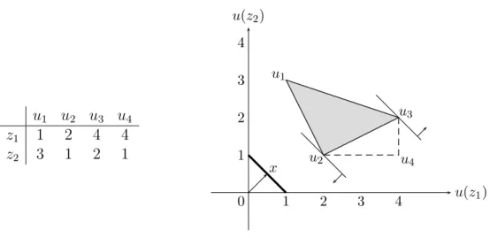
u1 u2 u3 u4 z1 1 2 4 4 z2 3 1 2 1 u(z1) u(z2) u4 u1 u2 x u3 0 1 2 3 4 1 2 3 4
Figure 2: Example of set of utility functions (continued)
are the socially most determinate social welfare functions satisfying Independence of Irrelevant Alternatives and Pareto Weak Preference.
Finally, let us briefly sketch the proof of the “only if” part of Theorem 2 (the proof of the “if” part is straightforward). Beforehand, it is useful to understand in more detail why a set of utility functions is only partially pinned down by all utility intervals. To this end, let us go back to the example that we considered in Figure 1 in Section 3. The definition of the four utility functions u1, u2, u3, u4 ∈ P on the set Z = {z1, z2} are recalled
in the left-hand side table of Figure 2. The right-hand side graph depicts these utility functions but this time in RZ rather than RX (this is possible, of course, since a vNM
utility function u ∈ P is fully determined by the vector (u(z1), u(z2)) ∈ RZ). The set
U = conv({u1, u2, u3}) of utility functions now corresponds to the shaded triangle u1u2u3.
The utility interval U(x) of alternative x ∈ X (the set X of alternatives is represented by the thick segment on the graph) can now be visualized as follows: max U(x) corresponds to the hyperplane supporting U in the (normal) direction x whereas min U(x) corresponds to the hyperplane supporting U in the direction −x.
Being essentially a compact and convex subset of RZ, a set of utility functions is fully
determined by its supporting hyperplanes in all directions of RZ. The utility intervals
of all alternatives, however, only determine these supporting hyperplanes in the non-negative and non-positive directions and, hence, do not fully pin down the set of utility functions. Thus, the set U′ = conv({u
1, u2, u3, u4}) of utility functions (corresponding
to the quadrilateral u1u2u3u4), although strictly larger than U, only differs from U in
directions with both positive and negative components and, hence, yields the same utility intervals as U for all alternatives.
Now for the proof sketch, first note that by Theorem 1, we know there exists a non-empty, compact, and convex set Φ ⊂ (RI
+)2×R such that (2) holds. In order to strengthen
satisfying Independence of Irrelevant Alternatives and Pareto Indifference that always yield the same social utility interval must always yield the same social utility set. Given our topological assumptions and since we restrict attention to vNM utilities, it turns out to be sufficient to show that F and F′ must always yield the same restriction of the social
utility set to any pair of alternatives.
So suppose there is a profile (Ui)i∈I ∈ D such that F ((Ui)i∈I)(x) = F′(Ui)i∈I(x) for
all x ∈ X but F ((Ui)i∈I)|{z1,z2} 6= F
′(U
i)i∈I|{z1,z2} for two outcomes z1, z2 ∈ Z. As we
just explained, F ((Ui)i∈I)|{z1,z2} and F
′(U
i)i∈I|{z1,z2} must then differ in some direction
of R{z1,z2} with both positive and negative components. For instance, F ((U
i)i∈I)|{z1,z2}
and F′(U
i)i∈I|{z1,z2}, may be the sets U and U
′ of the previous example, which differ in
the direction (2, −1) (among others), as 2u4(z1) − u4(z2) > 2u(z1) − u(z2) for all u ∈ U.
Take then an outcome z3 ∈ Z \ {z1, z2} and a profile ( ˜Ui)i∈I ∈ D that agrees with (Ui)i∈I
on {z1, z2} and such that ˜ui(z3) = 2˜ui(z1) − ˜ui(z2) for all ˜ui ∈ ˜Ui and all i ∈ I. By
Independence of Irrelevant Alternatives, we must then have F (( ˜Ui)i∈I)|{z1,z2} = U and
F′( ˜U
i)i∈I|{z1,z2} = U
′ and, by Pareto Indifference, we must also have ˜u(z
3) = 2˜u(z1)−˜u(z2)
for all ˜u ∈ F ((Ui)i∈I) ∪ F′((Ui)i∈I). Hence the above inequality yields F (( ˜Ui)i∈I)(z3) =
[3, 6] and 7 ∈ F′(( ˜U
i)i∈I)(z3), a contradiction.
5
General alternatives and domains
Up to now we have maintained two assumptions in order to simplify the exposition. First, the set of alternatives is a convex set of probability measures over some set Z of outcomes containing all probability measures on Z with finite support. Second, the domain of the social welfare function is the set of all profiles of (vNM) utility sets on X. Our results, however, also hold for other alternatives and domains. In this section we state general properties of the set of alternatives and the domain of the social welfare functions that are sufficient for our results and we discuss some particular settings in which these properties are satisfied.
First, we assume X is a mixture space, i.e. any set endowed with a mixing operation [0, 1] × X × X → X, (λ, x, y) 7→ xλy, such that for all x, y ∈ X and all λ, µ ∈ [0, 1], x1y = x, xλy = y(1 − λ)x, and (xλy)µy = x(λµ)y. Note that all definitions and axioms introduced so far have been stated with this general notation and, hence, apply to any mixture space.
Any convex set of probability measures over some set Z of outcomes is a mixture space, whether it contains all probability measures with finite support or not. Thus, besides all instances mentioned in Section 2, convex sets of probability measures with continuous or differentiable density are also mixture spaces. A somewhat different example, that has received recent attention in the literature, is the set of all compact and convex subsets of any of the above instances of mixture spaces, interpreted as menus (opportunity sets).
More generally, whenever X is a convex subset of some linear space, defining the mixing operation xλy = λx + (1 − λ)y by means of the vector addition and scalar multi-plication operations turns it into a mixture space. Such a mixture space, in addition, has the particular property that any pair of {x, y} ⊆ X of distinct alternatives is separated, i.e. for all r, s ∈ R there exists u ∈ P such that u(x) = r 6= u(y) = s. In fact, Mongin [18] shows that all pairs of distinct alternatives in X are separated if and only if there exists a mixture preserving bijection from X into a convex subset of some linear space (and that, moreover, the affine dimension of this subset is unique), and provides exam-ples of mixture spaces in which no, or some but not all, pairs of distinct alternatives are separated. Let us say, more generally, that a set Y ⊆ X is separated if, for all v ∈ RY,
there exists u ∈ P such that u|Y = v.5
Second, we introduce the following richness conditions on the domain of the social welfare function:
Definition 2. A domain D ⊆ PI is
• Indifference-rich if, for all x, y ∈ X and all (Ui)i∈I ∈ D such that Ui(x) = Ui(y) for
all i ∈ I, there exist z ∈ X and (U′
i)i∈I, (Ui′′)i∈I ∈ D such that Ui′|{x,z}= Ui′′|{y,z} =
{(γ, γ) : γ ∈ Ui(x) = Ui(y)} for all i ∈ I.
• Polygon-rich if, for all non-empty and finite (Vi)i∈I ⊂ (R2)I, there exist x, y ∈ X,
x 6= y, and (Ui)i∈I ∈ D such that Ui|{x,y} = conv(Vi) for all i ∈ I.
• Calibration-rich if, for all x, y ∈ X, all (Ui)i∈I ∈ D and all λ ∈ (0, 1), there exist
z ∈ X and (U′
i)i∈I ∈ D such that, for all i ∈ I, U′|{x,y} = U|{x,y}and u′i(x) = u′i(yλz)
for all u′ i ∈ Ui′.
In words, D is indifference-rich if, starting from any profile in D in which each individual has the same utility intervals for two alternatives x and y, we can always find a third alternative z as well as a second and a third profile in D in which each individual has the same utility interval for z as for x or y in the first profile and, furthermore, is indifferent between x and z in the second profile as well as between y and z in the third profile. D is polygon-rich if every profile of (convex hulls of) finite sets of pairs of utility levels (polygon) corresponds to the restriction of some profile in D to some pair of distinct alternatives. Finally, D is calibration-rich if, starting from any two alternatives x and y, any profile in D, and any coefficient λ strictly between 0 and 1, we can always find a third alternative z and a second profile in D having the same restriction to the pair {x, y} as the first profile and in which each individual is indifferent between x and yλz (by an appropriate calibration of the utility level of z).
5More precisely, Mongin [18] defines a pair {x, y} to be separated if there exists u ∈ P such that
Note that polygon-richness requires X to contain a separated pair of alternatives, and calibration-richness requires X to contain a separated triple of alternatives. If X is a non-empty and convex subset of some linear space (i.e. if all pairs of distinct alternatives in X are separated), then the full domain D is always indifference-rich, is polygon-rich whenever X contains a separated pair of alternatives (i.e. is of affine dimension at least one), and is calibration-rich whenever X contains a separated triple of alternatives (i.e. is of affine dimension at least two).
Technically, indifference-regularity is necessary for Independence of Irrelevant Alter-natives and Pareto Indifference to imply interval-neutrality (Lemma 1). Polygon-richness ensures that any profile of real intervals corresponds to the utility intervals of some alter-native in some profile in the domain, and also allows the construction of some particular profiles in the proof of Theorem 1. Calibration-richness is needed for the last step in the proof sketch of Theorem (4). Our results thus generalize as follows.
Proposition 1. Lemma 1 holds for any non-empty mixture space and any indifference-rich domain. Lemma 2 holds for any non-empty mixture space. Theorem 1 holds for mixture space containing a separated pair of alternatives and any polygon-rich domain. Theorem 2, Corollary 1, and Corollary 2 hold for any mixture space containing a separated triple of alternatives and any indifference-rich, polygon-rich, and calibration-rich domain.
6
Conclusion
This paper constitutes a first step towards extending social choice theory to situations in which individuals may have only partially determined preferences or utilities. Specifically, we adopt a standard multi-profile setting in which individuals are endowed with vNM utility functions and introduce indeterminacy by replacing vNM utility functions by sets of vNM utility functions, such a set representing the possible utility functions the individual may have, according to the social planner. Whereas it is known that for determinate utilities, basic axioms preclude all but utilitarian aggregation rules, it turns out that the class of rules satisfying natural generalizations of these axioms is much richer for indeterminate utilities. This class, and several subclasses (including the utilitarian class) can be characterized, although moving from determinate to indeterminate utilities raises several technical and conceptual issues.
One implication of our results is that in this settings, basic axioms entail some degree of social indeterminacy: as soon as one individual has indeterminate utility, so must have society. In other words, there is no possibility for the social planner to “resolve” individual indeterminacies, as could seem desirable. One possible way out of this impossibility could be to relax the vNM assumption on social preferences (allowing for a max-min criterion, for instance). More generally, it seems worthwhile investigating whether similar results
obtain when introducing indeterminacy in other social choice settings.
Appendix: proofs
We directly state the proofs in the general setting of Section 5.
Proof of Lemma 1
Assume X is a non-empty mixture space, D is an indifference-rich domain, and F satisfies Independence of Irrelevant Alternatives and Pareto Indifference. Let (Ui)i∈I, (Ui′)i∈I ∈ D
and x, y ∈ X such that Ui(x) = Ui′(y) for all i ∈ I. Since D is indifference-rich, there
exist z ∈ X and (U′
i)i∈I, (Ui′′)i∈I ∈ D such that Ui′|{x,z} = Ui′′|{y,z} = {(γ, γ) : γ ∈
Ui(x) = Ui(y)} for all i ∈ I. Hence F ((Ui)i∈I)(x) = F′((Ui)i∈I)(x) = F′((Ui)i∈I)(z) =
F′′((U
i)i∈I)(z) = F′′((Ui)i∈I)(y), where the first and third inequalities follow from
Inde-pendence of Irrelevant Alternatives and the second and fourth ones from Pareto Indiffer-ence.
Proof of Lemma 2
Assume X is a non-empty mixture space.
(a) Let U ∈ P, x, y ∈ X, and λ ∈ [0, 1]. Then by definition,
U(xλy) = {u(xλy) : u ∈ U}
= {λu(x) + (1 − λ)u(y) : u ∈ U} ⊆ {λu(x) + (1 − λ)v(y) : u, v ∈ U} = λU(x) + (1 − λ)U(y).
(b) Let U ∈ P, x, y ∈ X, and λ ∈ [0, 1]. Then by definition, there exist u, u′ ∈ U such
that u(x) = max U(x) and u′(y) = min U(y). Suppose λ max U(x) + (1 − λ) min U(y) >
max U(xλy). Then λ max U(x)+(1−λ) min U(y) > u(xλy) = λu(x)+(1−λ)u(y). Hence, since u(x) = max U(x), it must be that u(y) < min U(y), a contradiction since u ∈ U. Similarly, suppose λ max U(x) + (1 − λ) min U(y) < min U(xλy). Then λ max U(x) + (1 − λ) min U(y) < u′(xλy) = λu′(x) + (1 − λ)u′(y). Hence, since u′(y) = min U(y), it must
be that u′(x) > max U(x), a contradiction since u′ ∈ U.
Proof of Theorem 1
Assume X is a mixture space containing a separated pair of alternatives and D is an indifference-rich and polygon-rich domain. Clearly, if there exists a non-empty, compact, and convex set Φ ⊂ (RI
assume F is interval-neutral. Note that for a given non-empty, compact, and convex set Φ ⊂ (RI
+)2× R, (2) holds if and only if, for all (Ui)i∈I ∈ D and all x ∈ X,
max F ((Ui)i∈I)(x) = max (α,β,γ)∈Φ X i∈I αimax Ui(x) − X i∈I βimin Ui(x) + γ ! ,
min F ((Ui)i∈I)(x) = min (α,β,γ)∈Φ X i∈I αimin Ui(x) − X i∈I βimax Ui(x) + γ ! . (7)
Let K denote the set of all non-empty and compact real intervals. Since D is polygon-regular, for all (Ki)i∈I ∈ K I, there exist x ∈ X and (Ui)i∈I ∈ D such that Ui(x) = Ki
for all i ∈ I. Hence {(Ui(x))i∈I : (Ui)i∈I ∈ D, x ∈ X} = K I so, by interval-neutrality,
there exists a unique function G : K I → K such that, for all (U
i)i∈I ∈ D and all x ∈ X,
F ((Ui)i∈I)(x) = G((Ui(x))i∈I).
Let T = {(r, s) ∈ (RI)2 : ∀i ∈ I, r
i+ si ≥ 0}, and define the functions G, G : (RI)2 →
R ∪ {−∞, +∞} by, for all (r, s) ∈ (RI)2,
G(r, s) = max G(([−si, ri])i∈I) if (r, s) ∈ T, +∞ otherwise, G(r, s) = − min G(([−ri, si])i∈I) if (r, s) ∈ T, +∞ otherwise.
Clearly, dom(G) = dom(G) = T .6 Moreover, G(r, s) > −∞ and G(r, s) > −∞ for all
(r, s) ∈ (RI)2, so G and G are proper. Also note that, for all (r, s) ∈ T ,
G(r, s) + G(s, r) = max G(([−si, ri])i∈I) − min G(([−si, ri])i∈I) ≥ 0.
Finally, for all (Ui)i∈I ∈ D and all x ∈ X, we have
max F ((Ui)i∈I)(x) = max G((Ui(x))i∈I) = G((max Ui(x), − min Ui(x))i∈I),
min F ((Ui)i∈I)(x) = min G((Ui(x))i∈I) = −G((− min Ui(x), max Ui(x))i∈I),
so for a given non-empty, compact, and convex set Φ ⊂ (RI
+)2× R, (7) holds if and only
if, for all (r, s) ∈ T ,
G(r, s) = max
(α,β,γ)∈Φ(αr + βs + γ), G(r, s) = max(α,β,γ)∈Φ(αr + βs − γ). (8)
Lemma 3. G and G are convex.
Proof. We only state the proof for G, the argument for G is similar. Let (r, s), (r′, s′) ∈
T . Since D is polygon-rich, there exist x, y ∈ X, x 6= y, and (Ui)i∈I ∈ D such that
Ui|{x,y} = conv({wi, wi′}) for all i ∈ I, where wi, wi′ ∈ R{x,y} are defined by
wi(x) = −si, wi′(x) = ri,
wi(y) = −s′i, wi′(y) = ri′.
Note that for all i ∈ I and all λ ∈ [0, 1], we have Ui(xλy) = [−λsi−(1−λ)s′i, λri+(1−λ)ri′].
Hence, for all λ ∈ [0, 1],
G(λ(r, s) + (1 − λ)(r′, s′)) = G(λr + (1 − λ)r′, λs + (1 − λ)s′)
= max G(([−λsi− (1 − λ)s′i, λri+ (1 − λ)r′i])i∈I)
= max G((Ui(xλy))i∈I)
= max F ((Ui)i∈I)(xλy)
≤ λ max F ((Ui)i∈I)(x) + (1 − λ) max F ((Ui)i∈I)(y)
= λ max G((Ui(x))i∈I) + (1 − λ) max G((Ui(y))i∈I)
= λ max G(([−si, ri])i∈I) + (1 − λ) max G(([−s′i, r ′ i])i∈I)
= λG(r, s) + (1 − λ)G(r′, s′),
where the inequality follows from Lemma 2(a).
Lemma 4. G and G are non-decreasing.
Proof. We only state the proof for G, the argument for G is similar. It is sufficient to prove that for all i ∈ I, G is non-decreasing in (ri, si). So fix some i ∈ I and let
(r, s), (r′, s′) ∈ T such that (r′
i, s′i) ≥ (ri, si) and (r′j, s′j) = (rj, sj) for all j ∈ I \ {i}. We
proceed in two steps. First, we prove that G(r′, s′) ≥ G(r, s) whenever r
i+si > 0. To this
end, we assume without loss of generality that r′
i+s′i ≤ 2(ri+si). Since D is polygon-rich,
there exist x, y ∈ X, x 6= y, and (Uj)j∈I ∈ D such that Uj|{x,y} = conv({wj, wj′, wj′′, w′′′j })
for all j ∈ I, where wj, w′j, w′′j, wj′′′ ∈ R{x,y} are defined by
wj(x) = −s′j, w′j(x) = s′j− 2sj, wj′′(x) = r′j, wj′′′(x) = 2rj− rj′, wj(y) = s′j− 2sj, w′j(y) = −s ′ j, w ′′ j(y) = 2rj− rj′, w ′′′ j (y) = r ′ j.
Note that for all j ∈ I, we have Uj(x) = Uj(y) = [−s′j, rj′] and Uj(x12y) = [−sj, rj]. Hence,
G(r, s) = max G(([−sj, rj])j∈I)
= max F ((Uj)j∈I)(x12y)
≤ 12max F ((Uj)j∈I)(x) + 12max F ((Uj)j∈I)(y)
= 1
2max G((Uj(x))j∈I) + 1
2max G((Uj(y))j∈I)
= 12max G(([−s′j, rj′])j∈I) + 12 max G(([−s′j, rj′])j∈I)
= G(r′, s′),
where the inequality follows from Lemma 2(a).
Second, we prove that G(r′, s′) ≥ G(r, s) whenever r
i+ si = 0. To this end, suppose
G(r′, s′) < G(r, s). Clearly, it must then be that r′
i + s′i > 0. Since D is polygon-rich,
there exist x, y ∈ X, x 6= y, and (Uj)j∈I ∈ D such that Uj|{x,y} = conv({wj, w′j}) for all
j ∈ I, where wj, wj′ ∈ R{x,y} are defined by
wj(x) = −sj, wj′(x) = rj, wj(y) = −s′j, w ′ j(y) = r ′ j.
Note that for all j ∈ I and all λ ∈ [0, 1], we have Uj(xλy) = [−λsj− (1 − λ)s′j, λrj+ (1 −
λ)r′
j]. Hence,
max F ((Uj)j∈I)(x) = max G((Uj(x))j∈I)
= max G([−sj, rj])j∈I)
= G(r, s) > G(r′, s′)
= max G([−s′j, rj′])j∈I)
= max G((Uj(y))j∈I)
= max F ((Uj)j∈I)(y),
so there exists λ ∈ (0, 1) such that λ max F ((Uj)j∈I)(x) + (1 − λ) min F ((Ui)i∈I)(y) >
max F ((Uj)j∈I)(y). Moreover,
max F ((Uj)j∈I)(xλy) = max G((Uj(xλy))j∈I)
= max G([−λsj − (1 − λ)s′j, λrj+ (1 − λ)rj′])j∈I)
= G(λ(r, s) + (1 − λ)(r′, s′)) ≤ G(r′, s′)
= max F ((Uj)j∈I)(y),
where the inequality follows from the first step. It follows that λ max F ((Uj)j∈I)(x) +
Lemma 5. G and G are continuous.
Proof. We only state the proof for G, the argument for G is similar. By Lemma 3, G is upper semi-continuous since T is a polyhedral cone (Rockafellar [20, Theorem 10.2, Theorem 20.5]), so it is sufficient to prove that G is lower semi-continuous, i.e. that cl G = G.7 By definition, cl G ≤ G. Conversely, let (r, s) ∈ (RI)2. If (r, s) /∈ T then
cl G(r, s) = G(r, s) = +∞ since T is closed. If (r, s) ∈ T then let (r′, s′) ∈ (RI)2 such
that r′
i > ri and s′i > si for all i ∈ I. Then (r′, s′) belongs to the relative interior of
T and, hence, cl G(r, s) = limλ→0+G((1 − λ)(r, s) + λ(r
′, s′)) (Rockafellar [20, Theorem
7.5]). By Lemma 4, we have G(r, s) ≤ G((1 − λ)(r, s) + λ(r′, s′)) for all λ ∈ [0, 1] and,
hence, G(r, s) ≤ cl G(r, s).
Lemma 6. For all (r, s) ∈ T and all µ > 1, G(µ(r, s)) + G(µ(r, s)) ≤ µ(G(r, s) + G(r, s)).
Proof. Let (r, s) ∈ T and µ > 1. Since D is polygon-rich, there exist x, y ∈ X, x 6= y, and (Ui)i∈I ∈ D such that Ui|{x,y} = conv({wi, wi′}) for all i ∈ I, where wi, wi′ ∈ R{x,y}
are defined by
wi(x) = −µsi, w′i(x) = µri,
wi(y) = µsi, w′i(y) = −µri.
Note that for all i ∈ I, we have Ui(x) = [−µsi, µri], Ui(y) = [−µri, µsi], Ui(x12y) = {0},
Ui(xµ1(x12y)) = [−si, ri], and Ui(y1µ(x12y)) = [−ri, si]. Hence,
µ+1
2µ G(µ(r, s)) − µ−1
2µ G(µ(r, s)) = µ+1
2µ max F ((Ui)i∈I)(x) + µ−1
2µ min F ((Ui)i∈I)(y)
≤ max F ((Ui)i∈I)(xµ+12µ y)
= max F ((Ui)i∈I)(x1µ(x12y))
= G(r, s),
where the inequality follows from Lemma 2(b). Similarly,
µ−1
2µ G(µ(r, s)) − µ+1
2µ G(µ(r, s)) = µ−1
2µ max F ((Ui)i∈I)(x) + µ+12µ min F ((Ui)i∈I)(y)
≥ min F ((Ui)i∈I)(xµ−12µ y)
= min F ((Ui)i∈I)(y1µ(x12y))
= −G(r, s),
where the inequality follows again from Lemma 2(b). Hence,
G(r, s) + G(r, s) ≥ µ+12µ G(µ(r, s)) − µ−12µ G(µ(r, s)) − µ−12µ G(µ(r, s)) + µ+12µ G(µ(r, s))
= 1µ(G(µ(r, s)) + G(µ(r, s))),
so G(µ(r, s)) + G(µ(r, s)) ≤ µ(G(r, s) + G(r, s)).
Let G0+, G0+ : (RI)2 → R ∪ {−∞, +∞} denote the recession functions of G and G,
respectively, i.e. (Rockafellar [20, Theorem 8.5]) for all (r, s) ∈ (RI)2,
G0+(r, s) = lim µ→+∞ G(µ(r, s)) µ , G0 +(r, s) = lim µ→+∞ G(µ(r, s)) µ .
G0+ and G0+ are positively homogenous, proper convex functions by definition, and are
closed since G and G are closed. Also note that G0+ and G0+ are non-decreasing by
Lemma 4.
Lemma 7. dom(G0+) = T and G0+= G0+.
Proof. Let (r, s) ∈ (RI)2. If (r, s) /∈ T then, clearly, G0+(r, s) = G0+(r, s) = +∞. Hence
it is sufficient to show that if (r, s) ∈ T then limµ→+∞ G(µ(r,s))µ = limµ→+∞ G(µ(r,s))µ < +∞.
So let (r, s) ∈ T . Since G(µ(r,s))µ and G(µ(r,s))µ are non-decreasing functions of µ (Rockafellar [20, Theorem 23.1]), and since the sum of these two functions is bounded above by Lemma 6, we have limµ→+∞G(µ(r,s))µ < +∞ and limµ→+∞ G(µ(r,s))µ < +∞. Moreover, for all µ > 1,
defining x, y, Ui, wi, and w′i as in the proof of Lemma 6 yields
1
2G(µ(r, s)) − 1
2G(µ(r, s)) = 1
2 max F ((Ui)i∈I)(x) + 1
2 min F ((Ui)i∈I)(y)
∈ [min F ((Ui)i∈I)(x12y), max F ((Ui)i∈I)(x12y)]
= [−G(0, 0), G(0, 0)],
by Lemma 2(b), so −µ2G(0, 0) ≤ µ1G(µ(r, s)) − µ1G(µ(r, s)) ≤ 2µG(0, 0) and, hence, limµ→+∞ G(µ(r,s))µ = limµ→+∞ G(µ(r,s))µ .
Lemma 8. G, G, G0+, and G0+ are Lipschitzian.
Proof. We only state the proof for G and G0+, the argument for G and G0+ is similar.
First, for all (r, s) ∈ (RI)2, let T (r, s) = ((− min{−r
i, si}, max{−ri, si})i∈I). Note that
T (r, s) ∈ T for all (r, s) ∈ (RI)2 and T (r, s) = (r, s) for all (r, s) ∈ T . Define the function
g : (RI)2 → R ∪ {−∞, +∞} by, for all (r, s) ∈ (RI)2, g(r, s) = G(T (r, s)). Clearly,
dom(g) = (RI)2 and, for all (r, s) ∈ T , g(r, s) = G(r, s). Moreover, g is convex since, for
all (r, s), (r′, s′) ∈ (RI)2 and all λ ∈ [0, 1],
g(λ(r, s) + (1 − λ)(r′, s′)) = G − min{λ(−ri) + (1 − λ)(−r′i), λsi+ (1 − λ)s′i}, max{λ(−ri) + (1 − λ)(−ri′), λsi+ (1 − λ)s′i} ! i∈I
≤ G −(λ min{−ri, si} + (1 − λ) min{−r′i, s′i}), λ max{−ri, si} + (1 − λ) max{−r′i, s ′ i} ! i∈I
= G λ(− min{−ri, si}, max{−ri, si})i∈I +(1 − λ)(− min{−r′
i, s′i}, max{−r′i, s′i})i∈I
!
≤ λG((− min{−ri, si}, max{−ri, si})i∈I) +(1 − λ)G((− min{−ri′, s′i}, max{−r′i, s′i})i∈I)
= λg(r, s) + (1 − λ)g(r′, s′),
where the first inequality follows from Lemma 4 and the second one from Lemma 3. Now, suppose G is not Lipschitzian. Then g is not Lipschitzian either. Hence, since g is finite and convex, there must exist (r, s) ∈ (RI)2 such that g0+(r, s) = +∞ (Rockafellar [20,
Theorem 10.5]), i.e. G0+(T (r, s)) = +∞, a contradiction by Lemma 7. Finally, note
that for all (r, s) ∈ (RI)2, g0+(r, s) = G0+(T (r, s)) < +∞ by Lemma 7. Hence g0+ is
Lipschitzian since it is its own recession function (Rockafellar [20, Theorem 10.5]), so G0+ is Lipschitzian.
Lemma 9. For all (r, s), (r′, s′) ∈ (RI)2, if G0+′((r, s), (r′, s′)) = −G0+′((r, s), −(r′, s′))
then8 G0+′((r, s), (r′, s′)) = lim µ→+∞G ′ (µ(r, s), (r′, s′)) = lim µ→+∞−G ′ (µ(r, s), −(r′, s′)) = lim µ→+∞G ′(µ(r, s), (r′, s′)) = lim µ→+∞−G ′(µ(r, s), −(r′, s′)).
Proof. We only state the proof for G, the argument for G is similar, given Lemma 7. Let (r, s), (r′, s′) ∈ (RI)2. If (r, s) /∈ T then the lemma is trivially true (all directional
derivatives are equal to +∞), so assume (r, s) ∈ T . Then, by definition of G0+′, for all
ε > 0, there exists δ0 > 0 such that
G0+((r, s) + δ 0(r′, s′)) − G0+(r, s) δ0 ≤ G0+′((r, s), (r′, s′)) + ε and, hence, lim µ→+∞ G(µ(r, s) + µδ0(r′, s′)) − G(µ(r, s)) µδ0 ≤ G0+′((r, s), (r′, s′)) + ε.
8Given a function f and a point x ∈ dom(f ), f′(x, y) denotes the (one-sided) directional derivative
of f at x in direction y, i.e. f′(x, y) = lim δ→0+
f(x+δy)−f (x)
δ if x ∈ dom(f ) and f
Hence, for all ε > 0, there exist δ0 > 0 and µ0 > 1 such that, for all µ ≥ µ0,
G(µ(r, s) + µδ0(r′, s′)) − G(µ(r, s))
µδ0
≤ G0+′((r, s), (r′, s′)) + ε.
Moreover, since µ(r, s) + δ0(r′, s′) = (1 − 1µ)(µ(r, s)) + 1µ(µ(rs) + µδ0(r′, s′)), we have
G(µ(r, s) + δ0(r′, s′)) ≤ (1 − µ1)G(µ(r, s)) +µ1G(µ(rs) + µδ0(r′, s′))
by Lemma 3 and, hence,
G(µ(r, s) + δ0(r′, s′)) − G(µ(r, s)) δ0 ≤ G(µ(r, s) + µδ0(r ′, s′)) − G(µ(r, s)) µδ0 .
Hence, for all ε > 0, there exist δ0 > 0 and µ0 > 1 such that, for all µ ≥ µ0,
G(µ(r, s) + δ0(r′, s′)) − G(µ(r, s))
δ0
≤ G0+′((r, s), (r′, s′)) + ε
and, hence, for all δ ∈ (0, δ0),
G(µ(r, s) + δ(r′, s′)) − G(µ(r, s))
δ ≤ G0
+′((r, s), (r′, s′)) + ε
by Lemma 3 (Rockafellar [20, Theorem 23.1]). Hence, by definition of G′, for all ε > 0, there exists µ0 > 1 such that G
′
(µ(r, s), (r′, s′)) ≤ G0+′((r, s), (r′, s′)) + ε for all µ ≥ µ 0.
Now, assume G0+′((r, s), (r′, s′)) = −G0+′((r, s), −(r′, s′)). Then, by the preceding
paragraph, for all ε > 0, there exists µ0 > 1 such that, for all µ ≥ µ0,
G′(µ(r, s), (r′, s′)) − ε ≤ G0+′((r, s), (r′, s′)) = −G0+′((r, s), −(r′, s′)) ≤ −G′(µ(r, s), −(r′, s′)) + ε ≤ G(µ(r, s), (r′, s′)) + ε
(where the last inequality follows from Rockafellar [20, Theorem 23.1]), so we obtain limµ→+∞G ′ (µ(r, s), (r′, s′)) = lim µ→+∞−G ′ (µ(r, s), −(r′, s′)) = G0+′((r, s), (r′, s′)) by
passing to the limit as ε → 0+.
Let G∗, G∗ : (RI)2 → R ∪ {−∞, +∞} denote the conjugate functions of G and G,
respectively, i.e. for all (α, β) ∈ (RI)2,
G∗(α, β) = sup
(r,s)∈T
(αr + βs − G(r, s)), G∗(α, β) = sup
(r,s)∈T
Since G and G are closed proper convex functions, so are G∗ and G∗ (Rockafellar [20, Theorem 12.2]). Moreover, G∗ and G∗ are clearly bounded below since, for all (α, β) ∈ (RI)2, G∗(α, β) ≥ −G(0, 0) and G∗(α, β) ≥ −G(0, 0).
Let C = {(−η, −η) : η ∈ RI
+} ⊂ (RI−)2. Clearly, C is a non-empty, closed, and convex
cone containing no line and, moreover, we have C = T◦.9 Let L ⊂ (RI)2 be the set of
points where G0+ is differentiable. Clearly, cl(L) = T (Rockafellar [20, Theorem 25.5]),
so L is non-empty.10 Let E = {∇G0+(r, s) : (r, s) ∈ L} and M = cl(conv(E)). By
Lemmas 4 and 8, E is a non-empty and bounded subset of (RI
+)2 and, hence, M is a
non-empty, compact, and convex subset of (RI +)2.
Lemma 10. For all (α, β) ∈ M + C, G∗(α, β) + G∗(α, β) ≤ 0.
Proof. We claim that G∗(α, β) + G∗(α, β) ≤ 0 for all (α, β) ∈ E. If this is true then we have G∗(α, β) + G∗(α, β) ≤ 0 for all (α, β) ∈ M since G∗+ G∗ is closed (Rockafellar [20, Theorem 9.3]). Moreover, for all η ∈ RI
+, we have G ∗
(α − η, β − η) = sup(r,s)∈T(αr + βs − η(r+s)−G(r, s)) ≤ G∗(α, β) and G∗(α−η, β−η) = sup(r,s)∈T(αr+βs−η(r+s)−G(r, s)) ≤ G∗(α, β) since r + s ≥ 0 for all (r, s) ∈ T . Hence G∗(α, β) + G∗(α, β) ≤ 0 for all (α, β) ∈ M + C.
To prove the claim, let (α, β) ∈ E. Since G∗ and G∗ are closed, it is sufficient to find two sequences (αµ, βµ)µ≥1 and (αµ, βµ)µ≥1 in (RI)2 such that limµ→+∞(αµ, βµ) =
limµ→+∞(αµ, βµ) = (α, β) and limµ→+∞G ∗
(αµ, βµ) + limµ→+∞G∗(αµ, βµ) ≤ 0. Moreover,
since G∗ and G∗ are bounded below, a sufficient condition for limµ→+∞G ∗ (αµ, βµ) + limµ→+∞G∗(αµ, βµ) ≤ 0 is that G ∗ (αµ, βµ) + G ∗(α µ, βµ) ≤ 0 for all µ ≥ 1.
In order to construct these sequences, note that since (α, β) ∈ E, we have (α, β) = ∇G0+(r, s) for some (r, s) ∈ L by definition. Clearly, (r, s) must then belong to the
interior of T (Rockafellar [20, Corollary 25.1.1]). Hence, for all µ ≥ 1, µ(r, s) also belongs to the interior of T , so ∂G(µ(r, s)) is non-empty and compact (Rockafellar [20, Theorem 23.4]).11 It follows that there exists (α
µ, βµ) ∈ ∂G(µ(r, s)) such that G ′
(µ(r, s), −(r, s)) = −αµr − βµs since G
′
(µ(r, s), ·) is the support function of ∂G(µ(r, s)) (Rockafellar [20, Theorem 23.2, Theorem 23.4]). Hence we have G(µ(r, s)) + G∗(αµ, βµ) = µ(αµr + βµs)
(Rockafellar [20, Theorem 23.5]) and, hence,
G∗(αµ, βµ) = −G(µ(r, s)) − µG ′ (µ(r, s), −(r, s)) = −G(µ(r, s)) − µ lim ε↓0 G((µ − ε)(r, s)) − G(µ(r, s)) ε = lim ε↓0 (µ − ε)G(µ(r, s)) − µG((µ − ε)(r, s)) ε .
9Given a cone S, S◦ denotes the polar cone of S, i.e. S◦= {y : ∀s ∈ S, xy ≤ 0}. 10Given a set S, cl(S) denotes the closure of S.
11Given a function f and a point x, ∂f (x) denotes the subdifferential of f at x, i.e. ∂f (x) = {x∗ :
Similarly, there exists (αµ, βµ) ∈ ∂G(µ(r, s)) such that G∗(αµ, βµ) = lim ε↓0 (µ − ε)G(µ(r, s)) − µG((µ − ε)(r, s)) ε . Hence, G∗(αµ, βµ) + G∗(αµ, βµ) = lim ε↓0 (µ − ε)(G(µ(r, s)) + G(µ(r, s))) − µ(G((µ − ε)(r, s)) + G((µ − ε)(r, s))) ε ≤ 0
by Lemma 6. Moreover, G0+′((r, s), ·) is linear since (r, s) ∈ L (Rockafellar [20,
The-orem 25.2]) and, hence, (G′(µ(r, s), ·))µ≥1 and (G′(µ(r, s), ·))µ≥1 converge pointwise to
G0+′((r, s), ·) as µ → +∞ by Lemma 9. Since G0+′((r, s), ·) is the support function
of ∂G0+(r, s) = {(α, β)}, it follows that lim
µ→+∞(αµ, βµ) = limµ→+∞(αµ, βµ) = (α, β)
(Schneider [21, Theorem 1.8.11, Theorem 1.8.12]).
Lemma 11. dom(G∗) = dom(G∗) = M + C.
Proof. Since G∗ and G∗ are proper, we have M + C ⊆ dom(G∗) ∩ dom(G∗) by Lemma 10. Hence it is sufficient to prove that cl(dom(G∗)) = cl(dom(G∗)) = M + C. To this end, note that by definition of G∗, G0+, G∗, and G0+, we have
cl(dom(G∗)) = {(α, β) ∈ (RI)2
: ∀(r, s) ∈ (RI)2, αr + βs ≤ G0+(r, s)},
cl(dom(G∗)) = {(α, β) ∈ (RI)2 : ∀(r, s) ∈ (RI)2, αr + βs ≤ G0+(r, s)}
(Rockafellar [20, Corollary 13.2.1, Theorem 13.3]), so cl(dom(G∗)) = cl(dom(G∗)) by Lemma 7. Moreover, since dom(G0+) = T , we have 0+cl(dom(G∗)) = {(α, β) ∈ (RI)2 :
∀(r, s) ∈ T, αr + βs ≤ 0} = T◦ = C.12 Hence cl(dom(G∗)) contains no line, so
cl(dom(G∗)) = cl(conv(exp(cl(dom(G∗)))) + C)
(Rockafellar [20, Theorem 18.7]).13 Moreover, exp(cl(dom(G∗))) = E (Rockafellar [20,
Corollary 25.1.3]) and, hence, cl(dom(G∗)) = M + C since E is bounded (Rockafellar [20, Corollary 9.1.1]).
Let C′ = C × R
+ ⊂ (RI+)2 × R. Clearly, C′ is a non-empty, closed, and convex cone
containing no line. Let L, L ⊂ (RI)2be the sets of points where G and G are differentiable,
respectively. Clearly, cl(L) = cl(L) = T (Rockafellar [20, Theorem 25.5]), so L and L
12Given a set S, 0+Sdenotes the recession cone of S, i.e. 0+S = {y : ∀x ∈ S, ∀µ > 0, x + µy ∈ S}. 13Given a set S, exp(S) denotes the set of exposed points of S.
are non-empty. Let E = {∇G(r, s) : (r, s) ∈ L} and E = {∇G(r, s) : (r, s) ∈ L}. By Lemmas 4 and 8, E and E are non-empty and bounded subsets of (RI
+)2. Moreover,
we have E ⊆ dom(G∗) and E ⊆ dom(G∗) (Rockafellar [20, Theorem 23.5]) and, hence, the sets E′ = {(α, β, G∗(α, β)) : (α, β) ∈ E} and E′ = {(α, β, G∗(α, β)) : (α, β) ∈ E} are non-empty and bounded subsets of (RI
+)2 × R since G ∗
and G∗ are bounded below and above by Lemma 10. Hence the sets M′ = cl(conv(E′)) and M′ = cl(conv(E′)) are non-empty, compact, and convex subsets of (RI
+)2× R.
Lemma 12. For all non-empty, compact, and convex set Φ ⊂ (RI
+)2 × R, M ′
⊆ Φ ⊆ M′+ C′ if and only if, for all (r, s) ∈ T , G(r, s) = max
(α,β,γ)∈Φ(αr + βs − γ). Similarly,
for all non-empty, compact, and convex set Φ ⊂ (RI
+)2 × R, M′ ⊆ Φ ⊆ M′ + C′ if and
only if, for all (r, s) ∈ T , G(r, s) = max(α,β,γ)∈Φ(αr + βs − γ).
Proof. We only state the proof for G, the argument for G is similar. Since G is closed, it is the conjugate function of G∗ (Rockafellar [20, Theorem 12.2]), i.e. for all (r, s) ∈ T ,14
G(r, s) = sup
(α,β)∈dom(G∗)
(αr + βs − G∗(α, β)) = sup
(α,β,γ)∈epi(G∗)
(αr + βs − γ).
We now prove that epi(G∗) = M′+ C′. First, we clearly have 0+epi(G∗) ⊆ 0+dom(G∗) ×
R = C ×R. Moreover, since G∗ is bounded below, we have in fact 0+epi(G∗) ⊆ C ×R +=
C′. Conversely, since G∗(α − η, β − η) ≤ G∗(α, β) for all (α, β) ∈ dom(G∗) and all η ∈ RI +
(see the proof of Lemma 10), we have C′ ⊆ 0+epi(G∗). Hence 0+epi(G∗) = C′ and,
hence, epi(G∗) contains no line, so we have epi(G∗) = cl(conv(exp(epi(G∗))) + C′) since
G∗ is closed (Rockafellar [20, Theorem 18.7]). Moreover, exp(epi(G∗)) = E′ (Rockafellar [20, Corollary 25.1.2]) and, hence, epi(G∗) = M′ + C′ since E′ is bounded (Rockafellar
[20, Corollary 9.1.1]).
Thus, for all (r, s) ∈ T , we have G(r, s) = sup(α,β,γ)∈M′
+C′(αr + βs − γ). Hence,
since G is finite on T by definition and since M′ is compact, it must be that G(r, s) = sup(α,β,γ)∈M′(αr + βs − γ) = max
(α,β,γ)∈M′(αr + βs − γ). It follows that G(r, s) =
max(α,β,γ)∈Φ(αr + βs − γ) for all non-empty, compact, and convex set Φ ⊂ (RI
+)2× R such
that M′ ⊆ Φ ⊆ M′+ C′. For the converse, first assume that Φ 6⊆ M′+ C′, i.e. that there
exists (α0, β0, γ0) ∈ Φ\(M ′
+C′). Then, since M′+C′is closed and convex and contains no
line, there exists (r, s, t) ∈ (RI)2×R with t 6= 0 such that α
0r +β0s+γ0t > αr +βs+γt for
all (α, β, γ) ∈ M′+ C′. Clearly, it must then be that (r, s, t) ∈ C′◦= T ×R
−. Hence, if we let (r′, s′) = (r |t|, s |t|) ∈ T , we have α0r ′+β 0s′−γ0 > αr′+βs′−γ for all (α, β, γ) ∈ M ′ +C′, so sup(α,β,γ)∈Φ(αr′ + βs′− γ) > sup (α,β,γ)∈M′+C′(αr ′+ βs′ − γ) = G(r′, s′). Now, assume
that Φ ⊆ M′ + C′ but M′ 6⊆ Φ, i.e. that there exists (α
0, β0, γ0) ∈ M ′
\ Φ. Then there exists (α0, β0, γ0) ∈ E
′
\ Φ (Rockafellar [20, Theorem 18.6]) and, hence, there ex-ists (r, s, t) ∈ (RI)2 × R with t 6= 0 such that α
0r + β0s + γ0t > αr + βs + γt for