HAL Id: hal-02466907
https://hal.archives-ouvertes.fr/hal-02466907
Submitted on 4 Feb 2020HAL is a multi-disciplinary open access archive for the deposit and dissemination of sci-entific research documents, whether they are pub-lished or not. The documents may come from teaching and research institutions in France or abroad, or from public or private research centers.
L’archive ouverte pluridisciplinaire HAL, est destinée au dépôt et à la diffusion de documents scientifiques de niveau recherche, publiés ou non, émanant des établissements d’enseignement et de recherche français ou étrangers, des laboratoires publics ou privés.
Climate limitation at the cold edge: contrasting
perspectives from species distribution modelling and a
transplant experiment
Caroline Greiser, Kristoffer Hylander, Eric Meineri, Miska Luoto, Johan
Ehrlén
To cite this version:
Caroline Greiser, Kristoffer Hylander, Eric Meineri, Miska Luoto, Johan Ehrlén. Climate limita-tion at the cold edge: contrasting perspectives from species distribulimita-tion modelling and a transplant experiment. Ecography, Wiley, 2020, �10.1111/ecog.04490�. �hal-02466907�
www.ecography.org
ECOGRAPHY
Ecography
––––––––––––––––––––––––––––––––––––––––
© 2020 The Authors. Ecography published by John Wiley & Sons Ltd on behalf of Nordic Society Oikos
Subject Editor: Vigdis Vandvik Editor-in-Chief: Jens-Christian Svenning Accepted 4 December 2019
43: 1–11, 2020
doi: 10.1111/ecog.04490 43 1–11The role of climate in determining range margins is often studied using species distri-bution models (SDMs), which are easily applied but have well-known limitations, e.g. due to their correlative nature and colonization and extinction time lags. Transplant experiments can give more direct information on environmental effects, but often cover small spatial and temporal scales. We simultaneously applied a SDM using high-resolution spatial predictors and an integral projection (demographic) model based on a transplant experiment at 58 sites to examine the effects of microclimate, light and soil conditions on the distribution and performance of a forest herb, Lathyrus vernus, at its cold range margin in central Sweden. In the SDM, occurrences were strongly associ-ated with warmer climates. In contrast, only weak effects of climate were detected in the transplant experiment, whereas effects of soil conditions and light dominated. The higher contribution of climate in the SDM is likely a result from its correlation with soil quality, forest type and potentially historic land use, which were unaccounted for in the model. Predicted habitat suitability and population growth rate, yielded by the two approaches, were not correlated across the transplant sites. We argue that the ranking of site habitat suitability is probably more reliable in the transplant experiment than in the SDM because predictors in the former better describe understory conditions, but that ranking might vary among years, e.g. due to differences in climate. Our results suggest that L. vernus is limited by soil and light rather than directly by climate at its northern range edge, where conifers dominate forests and create suboptimal condi-tions of soil and canopy-penetrating light. A general implication of our study is that to better understand how climate change influences range dynamics, we should not only strive to improve existing approaches but also to use multiple approaches in concert. Keywords: boreal forest, canopy cover, demography, microclimate, range margin, soil
Introduction
Identifying the factors limiting species distributions and driving abundance patterns is a longstanding question in ecology (Brown 1984, Austin 2007, Elith and Leathwick 2009), that has become particularly crucial in predicting the effects of environmental
Climate limitation at the cold edge: contrasting perspectives from
species distribution modelling and a transplant experiment
Caroline Greiser, Kristoffer Hylander, Eric Meineri, Miska Luoto and Johan Ehrlén
C. Greiser (https://orcid.org/0000-0003-4023-4402) ✉ (caroline.greiser@su.se), K. Hylander (https://orcid.org/0000-0002-1215-2648), E. Meineri (https://orcid.org/0000-0001-8825-8986) and J. Ehrlén(https://orcid.org/0000-0001-8539-8967), Dept of Ecology, Environment and Plant Sciences, Stockholm Univ., Stockholm, Sweden. CG, KH and JE also at: Bolin Centre for Climate Research, Stockholm Univ., Stockholm, Sweden. EM also at: Aix Marseille Univ., Univ. of Avignon, CNRS, IRD, IMBE, Marseille, France. – M. Luoto, Dept of Geosciences and Geography, Univ. of Helsinki, Finland.
and climate change (Guisan and Thuiller 2005, Thuiller et al. 2008). Species distribution models (SDMs) are the most common approach to study range-wide species–environment relationships. In SDMs, presence and absence data of a spe-cies are correlated with environmental variables (Guisan and Zimmermann 2000, Franklin 2009). SDMs are relatively easy to implement and can cover larger geographic areas. Further, SDMs integrate effects over longer time periods and effects of rare but important environmental conditions, e.g. cold spells or droughts (Hargreaves et al. 2014, Lee-Yaw et al. 2016). However, several limitations of SDMs have been pointed out (Austin 2007, Schurr et al. 2012, Urban et al. 2016). For example, SDMs are based on the assumption that occur-rences are in equilibrium with current environmental condi-tions, although it is known that time lags in extinctions and colonisations are important in many systems (Schurr et al. 2007, Thuiller et al. 2014, but see Engler and Guisan 2009). SDMs are also correlative in nature and might thus yield incorrect estimates of the impact of climate if climatic ables are correlated to other unknown or unmeasured vari-ables (Wiens et al. 2009, Guisan et al. 2017). Further, SDMs are typically based on free-air climate conditions at a coarse resolution, failing to capture the near-ground microclimates experienced by many organisms (Lembrechts et al. 2018).
To overcome some of the problems associated with SDMs, transplant experiments (TEs) have been suggested as a way to identify the factors determining species distributions (Gaston 2003, Ehrlén and Morris 2015). Main advantages of TEs are that they do not assume equilibria, and that they can extend the environmental gradient to include also conditions where the species do not currently exist (Lee-Yaw et al. 2016). Another advantage is that TEs, if including multiple life stages, enable examination of the demographic mechanisms underlying responses, i.e. how environmental variables affect different vital rates (e.g. survival, seed germination). Lastly, TEs combined with manipulative treatments can break up natural correlations between environmental variables, thus overcoming a main dis-advantage with many types of correlative studies (Battisti et al. 2005). However, identifying range-limiting factors using TEs is challenging because experiments need to be replicated along sufficiently long gradients of relevant environmental factors, and maintained over a sufficiently long time to capture tem-poral variation in conditions. TEs have also often not included all life stages (Sheppard et al. 2014, Lembrechts et al. 2017; but see Töpper et al. 2018). This is problematic because species distributions might be limited by effects during any phase of the organism’s life cycle and only integrated measures of popu-lation performance, such as popupopu-lation growth rates, can tell us if survival is possible at a given site. Since SDMs and TEs have different strengths and constraints and usually examine patterns at different temporal and spatial scales, an important way to increase our understanding of the factors limiting spe-cies distributions should be to combine the two approaches. Yet, such simultaneous assessments have rarely been done (but see Lee-Yaw et al. 2016, Benito-Garzón et al. 2019).
One type of questions where the simultaneous use of both methods might be particularly advantageous is how climate
change affects range margins. Range margins are expected to shift in response to rising temperatures (Thuiller et al. 2005, Chen et al. 2011, Vilà-Cabrera et al. 2019), and shifts may be most pronounced at poleward range margins (Normand et al. 2009). Climate limitations can be direct, when the marginal climate coincides with a species’ physiological limit, but also indirect, acting via changes in vegetation, biotic interactions or soil conditions (Aerts 1997, Dixon 2015). For example, a climate-driven shift from deciduous to conifer-dominated forests along the southern border of the boreal forests can modify litter fall and soil conditions (Dickinson and Pugh 1974, Barbier et al. 2008, Geiger et al. 2012). Different for-est types and landforms also create considerable near-ground microclimate variation (Suggitt et al. 2011, De Frenne and Verheyen 2015, Greiser et al. 2018). Due to microclimatic heterogeneity one would expect a patchy advancing front tracking global warming (Hylander et al. 2015), where species at their cold edge would occupy sites with relatively warmer microclimates (Beauregard and De Blois 2016). Thus, large-scale biogeographical predictions at range margins, based on coarse-gridded climate data, might miss that some local pop-ulations perform well (Vilà-Cabrera et al. 2019).
In this study, we explored the factors determining the distribution and performance of a perennial forest herb,
Lathyrus vernus, at its cold range margin, using two
differ-ent approaches. First, we built a SDM using high-resolution microclimate maps, as well as information about other impor-tant drivers such as forest age and forest type, to explore how environmental factors were correlated with the distribution at a regional scale. Second, we carried out an extensive TE on 58 sites with contrasting microclimate, light and soil mois-ture. In this experiment, we included multiple life cycle stages and integrated the effects of environmental variables on plant vital rates observed during one year using a demographic integral projection model. To separate direct effects of cli-mate from indirect effects occurring via soil development, we included an experimental treatment with nutrient-rich soil. We asked three main questions: 1) which environmen-tal variables explain the distribution in a SDM framework? 2) Which environmental variables affect vital rates and popu-lation growth rates in the TE? 3) Is habitat suitability derived from the SDM correlated with the population growth rate from the TE? We predicted that L. vernus in the study area is climate-limited and therefore responds positively to direct and indirect benefits from warmer temperatures. Because the two approaches included predictors that were associated with the same aspects of habitat suitability, we expected the predic-tions of the two models to largely agree.
Material and methods
Study systemLathyrus vernus (Fabaceae) is a long-lived herb growing in
mesic forests on base- and nutrient-rich soils (Ehrlén and Lehtilä 2002, Mossberg and Stenberg 2003). It accumulates
resources in rhizomes during the growing season, overwinters belowground and flowers in spring before canopy closure. The purple flowers are pollinated by bumblebees. The seeds are dispersed over relatively short distances by abruptly open-ing fruits (Ehrlén 2002). The species occurs in central and northern Europe and ranges to the east of the Ural Mountains (Hultén and Fries 1986). In Sweden L. vernus has a south-ern and south-eastsouth-ern distribution and declines inland above 60°N, while occurring further up along the coastal regions and in some northern river valleys.
This study was carried out in a sharp transition zone sepa-rating the northern boreal forest from the southern mixed forest in central Sweden – Limes Norrlandicus (Fig. 1, Greiser et al. 2018). The area belongs to the humid cold-temperate zone with annual mean temperature ranging from ca 5°C in the south to 3°C in the north (SMHI 2017). Precipitation decreases from west (800 mm) to east (600 mm; SMHI 2017) and falls as snow during the winter months. Soil pH is high in the south-east and east of the area and decreases rapidly towards the northwest. The heavily man-aged forests are dominated by Norway spruce and Scots pine in the canopy layer and dwarf-shrubs, mosses and lichens in the field layer (Rydin et al. 1999). The proportion of decidu-ous trees is overall low (0–40%), decreasing towards the north-northwest, and reaching higher values (up to 100%) only locally on early-successional patches after selective thin-ning, and on richer soils. Human population density in the countryside and various agricultural practices have histori-cally been more prevalent towards south-southeast.
Species distribution model
The area used for the SDM spanned from 58° to 61°N and from 12 to 19°E and embraced parts of the cold range mar-gin of L. vernus. For the model, we considered only forested area (52 409 km2, Fig. 1). We modelled the distribution of
L. vernus by relating presence data to six environmental
vari-ables at the highest possible resolution: climate, light, pro-portion of conifers, forest age, bedrock pH class and soil moisture. Presence data were obtained from a citizen science database (<https://artportalen.se/>, accessed 16 January 2016). We used only observations from the period 2000 to 2016 with a minimum spatial accuracy of 50 m. We filtered out observations outside forests and lumped the remaining points to a maximum of one observation per 50 m grid cell (obtaining 556 presences). Pseudo-absence data were created by sampling 1000 forested background points at a distance of 1–50 km from any presence point.
We used growing degree days (GDD) as a (micro)climate variable derived from high-resolution topoclimate grids of Sweden (Meineri and Hylander 2017). Solar radiation (SR) in spring and summer was used as a proxy for light availabil-ity, and was a function of latitude and local topography (Fu and Rich 2002). We also included the proportion of coni-fers (SLU Forest Map 2010), assuming that it partly reflected local light availability, light seasonality and soil pH. As another estimate of site acidity, we used the pH of the under-lying bedrock, classified as base-rich, neutral or acidic (bed-rock map from Geological Survey of Sweden, SGU jordarter
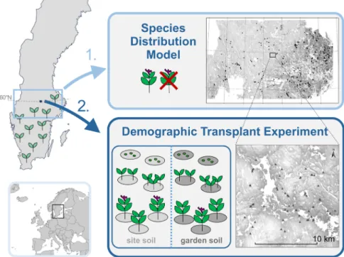
Figure 1. Study area and conceptual study design. Upper panel: first, we modelled the distribution of Lathyrus vernus across 52 409 km2 of
forested area at its cold range margin by relating presence–absence patterns to climate, light and soil variables. The map shows the presences as black dots. Lower panel: second, we tested in a transplant experiment the effects of climate, light and soil on the performance of L. vernus populations. The map shows the 58 transplant sites and schematic design of the experiment. At each site we planted adults, seedlings and seeds. Half of the plants at each site were planted in standard garden soil, half in original site soil.
vektor 1:25 000–1:10 000). We used the topographic wet-ness index (TWI) as an indirect measure for soil moisture (Sørensen et al. 2006). Lastly, to account for effects of land use we included forest age. Hypotheses for each variable are summarized in Table 1. All predictors were available as 50 m resolution raster files.
In the SDMs we used the following algorithms: gen-eralized linear models (GLM), gengen-eralized additive mod-els (GAM), boosted regression trees (generalized boosting models, GBM) and random forests (RF). These were com-bined in an ensemble model using the R package biomod2 (Thuiller et al. 2016). We used the true skill statistics (TSS, Allouche et al. 2006) and mean values of the area under the curve of a receiver operating characteristic plot to evaluate models (AUC, Fielding and Bell 1997). To assess the role of environmental variables, we computed their relative impor-tance (Thuiller et al. 2009) and response curves for each model (more model details in Supplementary material Appendix 1). Finally, we projected the habitat suitability for the entire area using only models with a TSS score > 0.55 and weighting their contribution proportional to their TSS scores with the default weight decay of 1.6 (Thuiller et al. 2010).
Transplant experiment
For the transplant experiment, we did a stratified random selection to identify 58 sites within a 16 × 16 km area in the centre of the area used for the SDM (Fig. 1). We considered
the following factors in the site selection: microclimate, forest type and age, soil type and moisture (Supplementary mate-rial Appendix 1). At each of the sites, we transplanted six adults, ten juveniles and 60 seeds across an area of 5 × 5 m (Fig. 1, Supplementary material Appendix 2 Fig. A2). To fur-ther examine the effect of soil, half of the plants were placed in original site soil, and the other half in garden soil, the lat-ter was expected to provide the betlat-ter growing conditions compared to the original site soil (Supplementary material Appendix 1 and 2 Fig. A1).
Adult plants for the transplant experiment were raised from seeds from ten different populations in 2011 and 2012 and thereafter grown in a common garden (Dahlberg 2016). Seeds and seedlings originated from seeds collected in 2015 from a population in south-central Sweden (59°14′N, 17°16′E). Part of the intact seeds were used to raise seedlings in the greenhouse in 2016, and the remaining seeds were sown directly at our sites. The transplantation of adults and juveniles was carried out in April and May 2016. Seeds were sown in late July 2016, corresponding to the time of natural seed dispersal.
In June 2016, we recorded size (stem diameter and length of shoots), flowering status (flowering versus non-flowering) and number of fruits for all transplanted individuals. In June 2017, we recorded survival, size, flowering status, number of fruits, number of seeds per fruit and number and size of the seedlings that had established from the seeds sown in the first year (Supplementary material Appendix 1). Recruitment
Table 1. Predictor variables, their mean, range and underlying model hypothesis. Distributions of SDM predictors were estimated from the raster-grids, whereas distributions of the TE predictors were calculated from the 58 sites. SDM = species distribution model, TE = transplant experiment.
Approach Variable Hypothesis Unit Min Mean Max
SDM growing degree days,
GDD at its cold range margin, the species prefers places with warm microclimate (= high GDD)
°C 751 1365 1658
SDM solar radiation at high latitudes with low sun angle
during spring, the species may avoid topographically shaded sites
MW h−1 m−2 0.45 0.66 0.77
SDM proportion of conifers species avoids pure conifer stands due to low litter/soil pH and dark forest floors in the spring
– 0 0.97 1
SDM pH bedrock species prefers base-rich soils acidic, neutral,
base rich – – –
SDM forest age species is not found on clear cuts and
not in very young forests, where it is outcompeted by fast-growing herbs
yr 0 54 170
SDM topographic wetness index species avoids very dry and very wet sites – 8 12 26
TE soil type species responses positively to the standard
garden soil and shows different responses to the other variables in the different soil types
garden soil,
site soil – – –
TE canopy penetrating light species prefers habitats with more
canopy openness % 23 44 78
TE soil moisture species avoids very dry and very wet sites volume % 11 29 60
TE growing degree days
(April + May) at its cold range margin, the species prefers places with warm microclimate (= high GDD)
°C 139 170 221
TE freezing degree days
probability was defined as the proportion of seeds sown in the first year that germinated the second year and were alive at the time of the recording. Growth was defined as the change in log-transformed size between two years, and size was defined as the sum of the products of basal area and length for each shoot ((diameter)2× π/4 × length).
At each transplant site we took canopy cover photos after canopy closure (June 2016). Light was estimated by extracting the average percentage of white pixels from five binary canopy cover photos using the software ImageJ 1.50b (Abràmoff et al. 2004). Soil moisture was measured in volume percent with a soil moisture meter (Delta-T Devices) at three locations per site during six dry days in September 2017. To adjust for dif-ferences among measurement days, moisture was also mea-sured at a reference site each day. We used the adjusted average of the three measurements as a site value. We recorded tem-perature at each site every 3 h with two iButton loggers (type DS1921G-F5 and DS1923, Maxim Integrated, San Jose, CA, USA), at 5 cm and 1 m height. Loggers were protected from direct sun and rain (Supplementary material Appendix 2 Fig. A3). Daily minimum (Tmin) and maximum temperatures (Tmax) were calculated from the average of the two loggers at each site. We extracted two complementary microclimate indices: spring growing degree days (GDD) that describes favour-ability of growing conditions, and spring freezing degree days (FDD) that describes harmful frost conditions (Choler 2017, Supplementary material Appendix 1). Before modelling, all predictors were checked for collinearity with the Spearman rank coefficient (no coefficient smaller or larger than ±0.50) and the variance inflation factor (no factor larger than 2). Vital rate models
We estimated the effects of GDD, FDD, light, soil moisture and soil type on five vital rates (survival, growth, probabil-ity of flowering, number of seeds produced and recruitment probability), using generalized linear mixed effect models and site as a random effect in the R package lme4 (Bates et al. 2015). For survival, probability of flowering and recruitment probability, which were binary distributed, we used logit link functions, and for growth and number of seeds (square-root transformed), which were normally distributed, we used identity links. We included size in year 2016 as a predictor for survival, and size in 2017 as a predictor for probability of flowering and number of seeds in 2017. A quadratic term for size was added in the growth function to allow for non-linear relationships between previous and current size.
The initial full models included the five environmental variables and all two-way interactions of the four continu-ous variables with soil type. Models were reduced stepwise using the drop1 function in R. Model terms were kept when residual deviance could be reduced significantly, using a Chi-square test for model comparison (Zuur et al. 2009). In order to avoid excluding potentially important effects of environmental variables in the IPM, we used a relatively liberal criterion of p < 0.1 for inclusion of model terms. All variables were standardized (z-transformed) before
modelling, and importance of each variable was inferred from standardized model coefficients of the final models. We calculated the goodness-of-fit (R2) for each model using the R package MuMIn (function r.squaredGLMM, Barton 2017), and extracted both the marginal R2, which includes only fixed effects, and the conditional R2, which includes both fixed and random effects.
Demographic model
Population growth rate, λ, was calculated using integral pro-jection models (IPMs), which are an advancement of classi-cal population matrix models, based on a continuous state variable rather than discrete classes (Easterling et al. 2000, Merow et al. 2014). We built an IPM for L. vernus based on standardized size as a state variable and the vital rate mod-els identified by statistical modmod-els (Supplementary material Appendix 1). We calculated lambda over the observed range of each continuous environmental variable (100 equal dis-tance levels), setting the other variables to their average. These calculations were done separately for both soil types. We compared the slopes of lambda over each environmental gra-dient to evaluate the impact on population growth rates. To assess the uncertainty of the lambda values, we bootstrapped the entire IPM-building procedure, including parametrizing the vital rate functions with the formula from the final model after model selection process. We bootstrapped a 100 times over sites with a sample size of 58 and assigned a pseudo-ID to each site-sample in order to be able to use the original for-mula with site as a random effect. Finally, we tested the corre-lation between predicted habitat suitability (log-transformed) from the SDM and population growth rates from the IPM, across the 58 sites and for both soil types.
All GIS work was done in ArcGIS ver. 10.4. All statistical analyses were done in R ver. 3.4.3 (R Core Team).
Results
Species distribution model
Habitat suitability for L. vernus decreased from SE to NW across the study area, and increased with higher GDD, lower proportion of conifers, older forests and higher pH (Fig. 2, Supplementary material Appendix 2 Fig. A5). GDD had the largest importance, followed by solar radiation, pH and pro-portion of conifers (Fig. 2). Habitat suitability was highest for low and high values of solar radiation. There was no clear cor-relation with TWI. The models had a good predictive qual-ity with mean TSS scores of 0.52 ± 0.007 SE and mean AUC scores of 0.81 ± 0.003 SE (Supplementary material Appendix 2 Fig. A4). Model quality varied among algorithms and were usu-ally slightly better for RF and GBM than for GLM and GAM. Transplant experiment
Plants survived, grew and germinated better in garden soil than in natural soil (Fig. 3, Supplementary material Appendix
2 Fig. A6, Table A1). The effect of other environmental fac-tors varied among vital rates, and differed between the two soil types. Light availability influenced survival and growth positively, but effects on growth were present only in garden soil. Higher soil moisture improved growth in both soils, but increased survival and tended to decrease the number of seeds and recruitment rate only in garden soil. FDD was positively related to survival in garden soil, and tended to be negatively related to the number of seeds. GDD tended to be positively correlated with growth in garden soil. All vital rates, except recruitment rate, increased significantly with increasing plant size (Supplementary material Appendix 2 Fig. A7). The vari-ance explained by the vital rate models was high for growth (conditional R2 = 0.80, marginal R2 = 0.75), moderate for survival (0.51, 0.26), probability of flowering (0.51, 0.34) and number of seeds (0.45, 0.27), but lower for recruitment (0.06, 0.04).
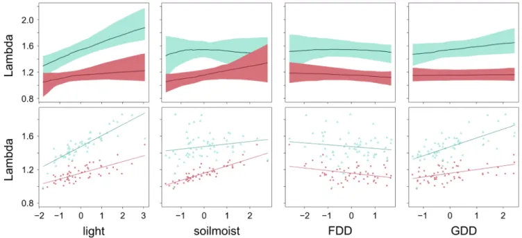
Integrating the environmental effects via all vital rates showed that soil type and light conditions had large and interactive effects on population growth rate (Fig. 4). Populations growing on sites with more light performed bet-ter, particularly when growing in garden soil. Soil moisture had a moderate positive effect on lambda in site soil, but no effect in garden soil. FDD decreased lambda slightly in both soils. GDD had a weak positive effect on lambda, but only in garden soil (Fig. 4).
Correlation between habitat suitability and population growth rate
Habitat suitability predicted by the SDM was not correlated with the estimated population growth rate across the 58 transplant sites (r = −0.15, p = 0.27 for site soil, and r = −0.19, p = 0.16 for garden soil, Fig. 5).
Discussion
In this study, we used two different approaches to examine the environmental factors that limit a southern forest herb at its cold range margin. The SDM identified a strong effect of climate, while in the TE light and soil had larger effects on population growth rate than climate. Although both mod-els agreed on the positive influence of warmer microclimate, there was no correlation between the predictions from the two approaches across the 58 sites. Below we discuss the results of each model, the reasons why results differed, and how the two approaches can complement each other.
Species distribution model
In concordance with the species’ reported ecology and our hypothesis, L. vernus occurrences correlated strongly with a warmer climate (more GDD), more base-rich bedrock, older forest and less conifer trees. Growing degree days was the strongest predictor, suggesting that the species currently is climate-limited at its northern range margin. This finding agrees with strong climatic signals reported from distribution
Figure 2. Examples of response curves (left) and relative importance (right) of five variables explaining presence/absence of L. vernus at its cold range margin using species distribution models. Relative importances are shown separately for each of the four model algo-rithms. Response curves are shown for the GAM models and observed predictor gradients (see main text for more details). Each colour in the response curve plots represents one of 15 separate model runs. GDD = growing degree days (base 5°C), SR = solar radiation in MW h−1 m−2, pH = pH class of bedrock, perccon =
pro-portion of conifers, TWI = topographic wetness index, GLM = gen-eralized linear model, GAM = generalized additive model, GBM = generalized boosting models, RF = random forest.
models of many other species. For example, Normand et al. (2009) found that half of the investigated vascular plants were limited by temperature at their latitudinal and altitu-dinal upper range margin. Beauregard and De Blois (2016) reported that some investigated plant species at their cold
edge shifted to sites with warmer microclimate conditions. Still, we are cautious to infer climate limitation from the cor-relative SDMs, since many environmental variables as well as land use history in our study area change in parallel with climate (Ashcroft et al. 2011).
Figure 3. Summary of the environmental factors in the vital rate models (survival, growth, probability of flowering, number of produced seeds, recruitment probability). Red = site soil, green and dashed = standard garden soil, black = main effect when interaction with soil type was not significant ‘.’ p < 0.1, ‘*’ p < 0.05, ‘**’ p < 0.01, ‘***’ p < 0.001, direction and steepness of slopes indicate direction and strength of effects. Soil = soil type: either site soil (red) or standard garden soil (green), light = canopy openness, soilmoist = soil moisture, FDD = freezing degree days, GDD = growing degree days. Regression coefficients are provided in Supplementary material Appendix 2 Table A1.
Figure 4. Effects of environmental factors (light, soil moisture, freezing degree days FDD, growing degree days GDD and their interaction with soil type) on the overall population growth rate measured as change in lambda, λ, over the observed range of one variable, while all others were set to their average. Light-green (triangles): standard garden soil. Red (circles): original site soil. All continuous variables are standardized. Upper panel: simulated lambda from bootstrapped models across all observed environmental gradients (median and 2.5th and 97.5th percentile). Lower panel: lambda for the 58 transplanted populations and imposed trend lines from single term linear regressions.
Transplant experiment
In contrast to most previous transplant experiments, our design enabled us to investigate the effects of relatively long gradients of microclimate, light and soil conditions. Moreover, our experiment included multiple life stages and allowed us to calculate integrated measures of the effects on population performance. This is important since different vital rates might react in opposed directions to environmental variables. For example, freezing conditions (low FDD) had a negative effect on survival, but a positive effect on number of produced seeds. Our results thus serve as an illustration of the importance of integrating effects on all vital rates in geographic range studies (Merow et al. 2017, Pironon et al. 2018). Similar to many previous experiments, our study was of relatively short duration, implying that the absolute esti-mates of long-term population performance are uncertain, and that inferences have to be based on relative performance differences across sites.
Garden soil had a strong positive effect on population growth rate. Interestingly, the effect of the other environmen-tal variables differed among soil types, being either weaker, as for soil moisture or stronger, as for light availability. This illustrates that interactive effects of environmental variables might often be important to understanding the factors deter-mining distributions (Ehrlén et al. 2016).
Light availability also had a strong effect on population growth rate via effects on survival and growth. Several previ-ous studies have shown that light availability may play a larger role than temperature gradients or nutrient availability on the forest floor (Flinn 2007, Baeten et al. 2010, De Frenne et al.
2015). Similarly, transplant experiments with other forest herbs have observed strong effects of soil and light conditions on plant performance (Meekins and McCarthy 2001, Van Der Veken et al. 2007). In boreal spruce-dominated forests, light conditions are likely to be particularly critical for light-demanding and early-flowering understory plants, because forest floors are dark and lack a shade-free period in the spring. Canopy-penetrating light is not only influencing photosyn-thetic active radiation, but also microclimate (Chen et al. 1993, Bramer et al. 2018, Greiser et al. 2018, Supplementary material Appendix 2 Fig. A8). A dense canopy buffers cold temperatures at night and warm temperatures during the day. Canopy cover also influences snow accumulation and ground frost during the winter (Storck et al. 2002).
Taken together, the results of the transplant experiment suggest that forest type, via effects on light and soil condi-tions, currently limit the species at its northern range margin and that direct effects of climate play a minor role. To the degree that climate controls the range of biomes and for-est tree composition, which in turn can alter soil and light regimes, it is possible that L. vernus is indirectly limited by climate. If deciduous species with a more open canopy in spring and a higher bark pH (e.g. maple, ash) will track the warming front, more sites may eventually become suitable for the species. Given that the pattern observed during this study holds true also for a longer time period and that the climate conditions in that period were representative, the experimen-tal populations seem to cope well with the climate at their current cold range margin.
How to reconcile the results of the two approaches? The results from the SDM and TE approaches appear con-vincing when viewed separately, but still they did not pro-duce a similar ranking of habitat quality across the 58 sites or a similar ranking of the importance of the environmental drivers. This might be associated with differences in both the predictors and the responses between the two models. Despite the fact that we used high-resolution spatial pre-dictors, the variables used to describe climate, light and moisture were not correlated between the two approaches (Supplementary material Appendix 2 Fig. A9). While we were able to get accurate on-site measures of soil moisture, understory light and microclimate in the transplant experi-ment, similar information was lacking in a mapped format for the SDM. Moreover, the lengths of environmental gra-dients differed between the two approaches (Table 1). While the range in light and soil quality across sites and between treatments were larger in the transplant experiment, differ-ences in climate variables were larger in the SDM. Taken together, this suggests that understory conditions were better described in the TE than in the SDM.
The SDM and the demographic TE also differed regarding the response against which the effects of environmental drivers were evaluated. The SDM predictions were based on occur-rence data (presences), which reflect environmental conditions over several decades, while estimated population growth rates
Figure 5. Relationship of population growth rate, lambda, derived from an integral projection model (IPM) and habitat suitability pre-dicted by a species distribution model (SDM) for 58 transplanted populations growing in either standard garden soil (light-blue tri-angles) or original site soil (red circles) in otherwise natural habitats with contrasting microclimate, moisture and soil conditions.
in the transplant experiment reflect current conditions, mea-sured during a single year. The SDM is thus more likely to have captured responses to long-term variation in important environmental drivers and rare events, like cold or dry years (but see Camarero et al. 2015), which can play an important role in determining cold range margins (Giesecke et al. 2010, Hargreaves et al. 2014, Lee-Yaw et al. 2016, Hoffmann et al. 2019). On the other hand, the long lifespan and poor disper-sal of the study species implies that distributions might not yet have tracked recent changes in habitat suitability, such as climate warming. Conversely, current population growth rates estimated by the TE should not suffer from time lags, but also do not capture the effects of rare events. An additional differ-ence is that while the SDM was based on natural populations, in the TE we used artificial populations where transplantation effects and planting design might have influenced performance. Based on all these differences in predictor and response vari-ables between the two approaches, it is reasonable to assume that they capture different temporal and spatial aspects of the species’ niche, and therefore, that their predictions could differ, but in informative and interpretable ways.
In line with this, the relatively high importance of soil type and moisture in the TE can be used to develop the interpre-tation of the SDM output, which captured well the gradient in habitat quality from southeast to northwest (Supplementary material Appendix 2 Fig. A5). This gradient is probably best represented by the climate variable, but also pH in the upper soil layer and the frequency of brown soils and deciduous for-est patches change in parallel (SLU Markinfo 2019). Thus, the apparent limiting effect of climate in the SDM might also reflect an effect of low soil quality due to acidifying litter and declining sub-canopy light availability in increasingly conifer-dominated stands. Even historic land use changes along this axis with the south-east having a higher proportion of land that was under the plough or mowed before 1900 (Bernes 2011). Effects of differences in land use history might be partly captured by current conditions, such as the presence of broadleaved trees (Cousins and Eriksson 2001). However, the historic land use could also have influenced the distribution of L. vernus in ways not captured by current conditions, such as dispersal via trans-port of hay (Auffret et al. 2014). To account for such effects in the SDM, we would need gridded layers of different historical land use types, which currently are unavailable.
Contrary to our expectations, we found no correlation between the predicted habitat suitability (SDM) and the estimated population growth rate (TE) across the 58 sites. We have provided several possible explanations for this lack of correlation and among many possible avenues for future studies, two important questions spur from this study. The first is under which conditions the rank order of popula-tion growth rates yielded in short-term TEs are representa-tive also of long-term growth rates. For example, while initial performance might have been driven largely by direct effects of environmental factors, the effects of competition might become increasingly important over time (Austin 1999). The second question is to what extent SDMs can be improved using a finer grid with better quality spatial predictors
(Potter et al. 2013, Lembrechts et al. 2018). Even if we used up-to-date high-resolution (50 m) predictors for several vari-ables, we still lacked high-resolution data, for example, on soil pH. Moreover, small-scale variation in light, soil mois-ture and understory microclimate appeared not to have been well captured by our data.
To mitigate some of the problems associated with SDMs several approaches have been suggested to also incorporate vital rates and dispersal rates into these models (e.g. dynamic range models – Schurr and Pagel 2012, Schurr et al. 2012, and hybrid models – Thuiller et al. 2008, Dullinger et al. 2012). Another suggested approach is to use population growth and dispersal rates to predict distributions (Merow et al. 2011). While these and similar approaches are basically attempts to integrate multiple processes in a single modelling frame-work, the main point illustrated by our study is that results obtained through different approaches can provide comple-mentary information leading to partly different inferences.
The relative strength and weaknesses of each approach will vary among study systems (Araújo and Peterson 2012, Schurr et al. 2012, Ehrlén and Morris 2015). For example, SDMs will be relatively more advantageous when environ-mental conditions are stationary, i.e. constant or stochasti-cally varying, and when rare climatic events, unlikely to be captured during a transplant experiment, are important. On the other hand, TEs are likely to provide more accurate information when environmental conditions are changing, because time lags in responses to changes will be smaller for population growth rates than for extinctions and coloniza-tions. SDMs are also likely to be particularly problematic for long-lived and poor-dispersed species, where we expect extinction and colonization time lags to be considerable. Lastly, from a methodological perspective, SDMs will be rela-tively more advantageous when information about putative environmental drivers is available in a mapped form and at a high spatial resolution, while TEs will be more useful when drivers are difficult to extract from map-based information. Data availability statement
Plant demographic data and site data are available at <https:// doi.org/10.5061/dryad.8931zcrm8> (Greiser et al. 2019).
Acknowledgements – The authors thank Daniela Guasconi, Simone
Moras, Sonia Merinero, Benny Willman and Giulia Zacchello for assisting in field, Johan Dahlgren for helping with the IPM, Hildred Crill for valuable comments on the manuscript and Sveaskog for allowing the transplant experiment on their property. Thanks also to two anonymous reviewers and the subject editor for improving the manuscript.
Funding – This research was funded by a FORMAS project grant
2014-530 (to KH).
Author contributions – JE, KH and CG conceived the ideas and
designed methodology; CG collected and analysed the data with support from all other authors; CG led the writing of the manuscript. All authors contributed critically to the drafts and gave final approval for publication.
References
Abràmoff, M. D. et al. 2004. Image processing with ImageJ. – Bio-photonics Int. 11: 36–41.
Aerts, R. 1997. Climate, leaf litter chemistry and leaf litter decom-position in terrestrial ecosystems: a triangular relationship. – Oikos 79: 439–449.
Allouche, O. et al. 2006. Assessing the accuracy of species distribu-tion models: prevalence, kappa and the true skill statistic (TSS). – J. Appl. Ecol. 43: 1223–1232.
Araújo, M. B. and Peterson, A. T. 2012. Uses and misuses of bioclimatic envelope modeling. – Ecology 93: 1527–1539. Ashcroft, M. B. et al. 2011. An evaluation of environmental factors
affecting species distributions. – Ecol. Model. 222: 524–531. Auffret, A. G. et al. 2014. The geography of human-mediated
dispersal. – Diversity 20: 1450–1456.
Austin, M. P. 1999. A silent clash of paradigms: some inconsisten-cies in community ecology. – Oikos 86: 170–178.
Austin, M. 2007. Species distribution models and ecological theory: a critical assessment and some possible new approaches. – Ecol. Model. 200: 1–19.
Baeten, L. et al. 2010. Plasticity in response to phosphorus and light availability in four forest herbs. – Oecologia 163: 1021–1032.
Barbier, S. et al. 2008. Influence of tree species on understory veg-etation diversity and mechanisms involved – a critical review for temperate and boreal forests. – For. Ecol. Manage. 254: 1–15.
Barton, K. 2017. MuMIn: multi-model inference. – R package ver. 1.40.0, <https://CRAN.R-project.org/package=MuMIn>. Bates, D. et al. 2015. Fitting linear mixed-effects models using
lme4. – J. Stat. Softw. 67: 1–48.
Battisti, A. et al. 2005. Expansion of geographic range in the pine processionary moth caused by increased winter temperatures. – Ecol. Appl. 15: 2084–2096.
Beauregard, F. and De Blois, S. 2016. Rapid latitudinal range expansion at cold limits unlikely for temperate understory forest plants. – Ecosphere 7: 1–17.
Benito-Garzón, M. et al. 2019. ΔTraitSDM: species distribution models that account for local adaptation and phenotypic plas-ticity. – New Phytol. 222: 1757–1765.
Bernes, C. 2011. Biodiversity in the agricultural landscape. – In: Bernes, C. (ed.), Biodiversity in Sweden. Swedish Environmen-tal Protection Agency, Monitor 22, pp. 120–165.
Bramer, I. et al. 2018. Advances in monitoring and modelling cli-mate at ecologically relevant scales. – Next Gener. Biomonit. Part 1 58: 1–61.
Brown, J. H. 1984. On the relationship between abundance and distribution of species. – Am. Nat. 124: 255–279.
Camarero, J. J. et al. 2015. Know your limits? Climate extremes impact the range of Scots pine in unexpected places. – Ann. Bot. 116: 917–927.
Chen, J. et al. 1993. Contrasting microclimates among clearcut, edge and interior of old-growth Douglas-fir forest. – Agric. For. Meteorol. 63: 219–237.
Chen, I. et al. 2011. Rapid range shifts of species associated with high levels of climate warming. – Science 333: 1024–1026. Choler, P. 2017. Winter soil temperature dependence of alpine
plant distribution: Implications for anticipating vegetation changes under a warming climate. – Perspect. Plant Ecol. Evol. Syst. 30: 6–15.
Cousins, S. A. O. and Eriksson, O. 2001. Plant species occurrences in a rural hemiboreal landscape: effects of remnant habitats, site history, topography and soil. – Ecography 24: 461–470. Dahlberg, C. J. 2016. The role of microclimate for the performance
and distribution of forest plants. – PhD thesis, Stockholm Univ. De Frenne, P. and Verheyen, K. 2015. Weather stations lack forest
data. – Science 351: 234.
De Frenne, P. et al. 2015. Light accelerates plant responses to warm-ing. – Nat. Plants 1: 15110.
Dickinson, C. H. and Pugh, G. J. F. 1974. Biology of plant litter decomposition. Volume 1. – Academic Press.
Dixon, J. C. 2015. Soil morphology in the critical zone: the role of climate, geology and vegetation in soil formation in the critical zone. – Elsevier.
Dullinger, S. et al. 2012. Extinction debt of high-mountain plants under twenty-first-century climate change. – Nat. Clim. Change 2: 619–622.
Easterling, M. R. et al. 2000. Size-specific sensitivity: applying a new structured population model. – Ecology 81: 694–708. Ehrlén, J. 2002. Assessing the lifetime consequences of plant–
animal interactions for the perennial herb Lathyrus vernus (Fabaceae). – Perspect. Plant Ecol. Evol. Syst. 5: 145–163. Ehrlén, J. and Lehtilä, K. 2002. How perennial are perennial plants?
– Oikos 98: 308–322.
Ehrlén, J. and Morris, W. F. 2015. Predicting changes in the distri-bution and abundance of species under environmental change. – Ecol. Lett. 18: 303–314.
Ehrlén, J. et al. 2016. Advancing environmentally explicit struc-tured population models of plants. – J. Ecol. 104: 292–305. Elith, J. and Leathwick, J. R. 2009. Species distribution models:
ecological explanation and prediction across space and time. – Annu. Rev. Ecol. Evol. Syst. 40: 677–697.
Engler, R. and Guisan, A. 2009. MigClim: predicting plant distri-bution and dispersal in a changing climate. – Divers. Distrib. 15: 590–601.
Fielding, A. H. and Bell, J. F. 1997. A review of methods for the assessment of prediction errors in conservation presence/absence models. – Environ. Conserv. 24: 38–49.
Flinn, K. M. 2007. Microsite-limited recruitment controls fern colo-nization of post-agricultural forests. – Ecology 88: 3103–3114. Franklin, J. 2009. Mapping species distributions: spatial inference
and prediction. – Cambridge Univ. Press.
Fu, P. and Rich, P. 2002. A geometric solar radiation model with applications in agriculture and forestry. – Comput. Electron. Agric. 37: 25–35.
Gaston, K. J. 2003. The structure and dynamics of geographic ranges. – Oxford Univ. Press.
Geiger, R. et al. 2012. The climate near the ground. – Springer Science and Business Media.
Giesecke, T. et al. 2010. The effect of past changes in inter-annual temperature variability on tree distribution limits. – J. Biogeogr. 37: 1394–1405.
Greiser, C. et al. 2018. Monthly microclimate models in a managed boreal forest landscape. – Agric. For. Meteorol. 250–251: 147–158.
Greiser, C. et al. 2019. Data from: Climate limitation at the cold edge – contrasting perspectives from species distribution mod-elling and a transplant experiment. – Dryad Digital Repository, <https://doi.org/10.5061/dryad.8931zcrm8>.
Guisan, A. and Zimmermann, N. E. 2000. Predictive habitat dis-tribution models in ecology. – Ecol. Model. 135: 147–186.
Guisan, A. and Thuiller, W. 2005. Predicting species distribution: offering more than simple habitat models. – Ecol. Lett. 8: 993–1009.
Guisan, A. et al. 2017. Habitat suitability and distribution models: with applications in R. – Cambridge Univ. Press.
Hargreaves, A. L. et al. 2014. Are species’ range limits simply niche limits writ large? A review of transplant experiments beyond the range. – Am. Nat. 183: 157–173.
Hoffmann, W. A. et al. 2019. Rare frost events reinforce tropical savanna-forest boundaries. – J. Ecol. 107: 468–477.
Hultén, E. and Fries, M. 1986. Atlas of north European vascular plants north of the Tropic Cancer. – Koeltz Scientific.
Hylander, K. et al. 2015. Microrefugia: not for everyone. – Ambio 44: 60–68.
Lee-Yaw, J. A. et al. 2016. A synthesis of transplant experiments and ecological niche models suggests that range limits are often niche limits. – Ecol. Lett. 19: 710–722.
Lembrechts, J. J. et al. 2017. Microclimate variability in alpine eco-systems as stepping stones for non-native plant establishment above their current elevational limit. – Ecography 40: 1–9. Lembrechts, J. J. et al. 2018. Incorporating microclimate into
spe-cies distribution models. – Ecography 24: 1267–1279. Meekins, J. F. and McCarthy, B. C. 2001. Effect of environmental
variation on the invasive success of a nonindigenous forest herb. – Ecol. Appl. 11: 1336–1348.
Meineri, E. and Hylander, K. 2017. Fine-grain, large-domain cli-mate models based on clicli-mate station and comprehensive top-ographic information improve microrefugia detection. – Ecog-raphy 40: 1003–1013.
Merow, C. et al. 2011. Developing dynamic mechanistic species distribution models: predicting bird-mediated spread of inva-sive plants across northeastern North America. – Am. Nat. 178: 30–43.
Merow, C. et al. 2014. Advancing population ecology with integral projection models: a practical guide. – Methods Ecol. Evol. 5: 99–110.
Merow, C. et al. 2017. Climate change both facilitates and inhibits invasive plant ranges in New England. – Proc. Natl Acad. Sci. USA 114: E3276–E3284.
Mossberg, B. and Stenberg, L. 2003. Den nya Nordiska floran. – Wahlström and Widstrand.
Normand, S. et al. 2009. Importance of abiotic stress as a range-limit determinant for European plants: insights from species responses to climatic gradients. – Global Ecol. Biogeogr. 18: 437–449.
Pironon, S. et al. 2018. The ‘Hutchinsonian niche’ as an assemblage of demographic niches: implications for species geographic ranges. – Ecography 41: 1103–1113.
Potter, K. A. et al. 2013. Microclimatic challenges in global change biology. – Global Change Biol. 19: 2932–2939.
Rydin, H. et al. 1999. Swedish plant geography. – Acta Phytogeogr. Suec. 84: 1–238.
Schurr, F. M. and Pagel, J. 2012. Forecasting species ranges by statistical estimation of ecological niches and spatial population dynamics. – Global Ecol. Biogeogr. 21: 293–304.
Schurr, F. M. et al. 2007. Colonization and persistence ability explain the extent to which plant species fill their potential range. – Global Ecol. Biogeogr. 16: 449–459.
Schurr, F. M. et al. 2012. How to understand species’ niches and range dynamics: a demographic research agenda for biogeogra-phy. – J. Biogeogr. 39: 2146–2162.
Sheppard, C. S. et al. 2014. Predicting plant invasions under cli-mate change: are species distribution models validated by field trials ? – Global Change Biol. 20: 2800–2814.
SLU Forest Map 2010. – Dept of Forest Resource Management, Swedish Univ. of Agricultural Sciences (SLU), <ftp://salix.slu. se/download/skogskarta/>, accessed 15 March 2015.
SLU MarkInfo 2019. – Swedish Forest Soil Inventory, with respon-sibility in the Dept of Soil and Environment, Swedish Univ. of Agricultural Sciences (SLU), <www.slu.se/miljoanalys/statistik-och-miljodata/miljodata/webbtjanster-miljoanalys/markinfo/ markinfo/kartor/>, accessed 10 January 2019.
SMHI 2017 Klimatdata. Database: dataserier med normalvärden för perioden 1961–1990. – Swedish Meteorological and Hydro-logical Inst., <www.smhi.se/klimatdata/>, accessed 20 March 2017.
Sørensen, R. et al. 2006. On the calculation of the topographic wetness index: evaluation of different methods based on field observations. – Hydrol. Earth Syst. Sci. 10: 101–112.
Storck, P. et al. 2002. Measurement of snow interception and can-opy effects on snow accumulation and melt in a mountainous maritime climate, Oregon, United States. – Water Resour. Res. 38: 1223–1239.
Suggitt, A. J. et al. 2011. Habitat microclimates drive fine-scale variation in extreme temperatures. – Oikos 120: 1–8.
Thuiller, W. et al. 2005. Climate change threats to plant diversity in Europe. – Proc. Natl Acad. Sci. USA 102: 8245–8250. Thuiller, W. et al. 2008. Predicting global change impacts on plant
species’ distributions: future challenges. – Perspect. Plant Ecol. Evol. Syst. 9: 137–152.
Thuiller, W. et al. 2009. BIOMOD – a platform for ensemble fore-casting of species distributions. – Ecography 32: 369–373. Thuiller, W. et al. 2010. Presentation manual for BIOMOD.
– Laboratoire d’Ecologie Alpine, Univ. Joseph Fourier. Thuiller, W. et al. 2014. Does probability of occurrence relate to
population dynamics? – Ecography 37: 1155–1166.
Thuiller, W. et al. 2016. biomod2: ensemble platform for species distribution modeling. – <https://cran.r-project.org/package= biomod2>.
Töpper, J. P. et al. 2018. The devil is in the detial: non-additive and context dependent plant population responses to increasing temperature and precipitation. – Global Change Biol. 24: 4657–4666.
Urban, M. C. et al. 2016. Improving the forecast for biodiversity under climate change. – Science 353: aad8466.
Van Der Veken, S. et al. 2007. Over the (range) edge: a 45-year transplant experiment with the perennial forest herb
Hyacinthoides non-scripta. – J. Ecol. 95: 343–351.
Vilà-Cabrera, A. et al. 2019. Refining predictions of population decline at species rear edges. – Global Change Biol. 25: 1549–1560.
Wiens, J. A. et al. 2009. Niches, models and climate change: assess-ing the assumptions and uncertainties. – Proc. Natl Acad. Sci. USA 106: 19729–19736.
Zuur, A. F. et al. 2009. Mixed effects models and extensions in ecology with R. – Springer.
Supplementary material (available online as Appendix ecog-04490 at <www.ecography.org/appendix/ecog-ecog-04490>). Appendix 1–2.