HAL Id: tel-01982526
https://tel.archives-ouvertes.fr/tel-01982526
Submitted on 15 Jan 2019HAL is a multi-disciplinary open access archive for the deposit and dissemination of sci-entific research documents, whether they are pub-lished or not. The documents may come from teaching and research institutions in France or abroad, or from public or private research centers.
L’archive ouverte pluridisciplinaire HAL, est destinée au dépôt et à la diffusion de documents scientifiques de niveau recherche, publiés ou non, émanant des établissements d’enseignement et de recherche français ou étrangers, des laboratoires publics ou privés.
products : Methodological development and application
to a perennial cropping system
Sandra Payen
To cite this version:
Sandra Payen. Toward a consistent accounting of water as a resource and a vector of pollution in the LCA of agricultural products : Methodological development and application to a perennial cropping system. Earth Sciences. Université Montpellier, 2015. English. �NNT : 2015MONTS119�. �tel-01982526�
Délivré par l’Université de Montpellier
Préparée au sein de l’école doctorale GAIA : Biodiversité,
Agriculture, Alimentation, Environnement, Terre, Eau
Et de l’unité de recherche Hortsys
Spécialité : Science de la Terre et de l’Eau
Présentée par Sandra PAYEN
Directeur de thèse : Mr Sylvain PERRET, HDR, Cirad
Soutenue le 16 Décembre 2015 devant le jury composé de
Mme Cécile BULLE, Professeure, CIRAIG Rapportrice
Mr Patrick DURAND, Directeur de recherche, INRA Rapporteur Mme Claudine BASSET-MENS, HDR, Cirad
Mr Christian GARY, Directeur de recherche, INRA
Examinatrice Examinateur Mr Mustapha ZEMZAMI, PhD, Les Domaines Agricoles Invité
Mr Vincent COLOMB, Ingénieur, ADEME Invité
Toward a consistent accounting of water as a
resource and a vector of pollution in the LCA of
agricultural products:
Methodological development and application to
a perennial cropping system
Remerciements
Tant de personnes ont contribué à l’accomplissement de ce travail. Je tiens à leur exprimer toute ma gratitude.
Merci aux hydrologues du LISAH, aux ACViste d’ELSA et d’ailleurs, au Docteur Ragab, au Professeur Fereres pour toutes ces discussions passionnantes qui donnent envie de faire plusieurs thèses…
Merci à Arnaud qui m’a donnée goût à l’ACV il y a déjà 7 ans,
Merci à Henri qui m’a enseigné tant de choses sur les agrumes et les manguiers, Merci à Sylvain pour ses conseils incroyablement pertinents,
Merci à Pauline pour son aide precieuse en un temps record, Et merci à mes chers amis pour leur soutien sans faille…
Enfin, je souhaite remercier ceux sans qui cette thèse n’aurait jamais vu le jour: mes parents, sans qui rien n’aurait été possible, et Claudine, source d’énergie et d’inspiration.
Bien plus important que le diplôme qu’elle confère, la thèse est une experience de vie incroyablement intense et instructive. J’ai beaucoup appris sur la science, la recherche, mais surtout sur moi-même. Tout cela grace à l’Echange. La communication en est la clef, et les relations humaines y sont centrales et essentielles. Merci à vous tous, car vous m’avez aidé à me construire.
Je souhaite dédier ma thèse à celle qui n’aura pas pu la suivre jusqu’au bout, mais qui me suit depuis là-haut.
Encadrement & financements
Ce travail a été co-encadré par Sylvain Perret (directeur de thèse) et Claudine Basset-Mens (co-directrice de thèse).
Cette thèse a été co-financée par l’ADEME (Agence de l’Environnement et de la Maitrise de l’Energie) et le CIRAD (Centre de coopération Internationale en Recherche Agronomique pour le Développement). La chaire industrielle ELSA-Pact et les Domaines Agricoles du Maroc ont notamment financés les missions de collecte des données et de communication des résultats.
Le suivi scientifique par un ingénieur de l’ADEME a été assuré par Vincent Colomb.
Table des matières
INTRODUCTION ... 2
WHY DOING LIFE CYCLE ASSESSMENT OF AGRICULTURAL SYSTEMS?
1.1.FEEDING THE PLANET WITHOUT DESTROYING IT ... 21.1.1. Agriculture is feeding the planet, but has many impacts on the environment ... 2
1.1.2. An increasing pressure…... 2
1.1.3. Identify the environmental hot spots and mitigation options ... 3
1.2.LCA OF AGRICULTURAL SYSTEMS: CHALLENGES ... 3
1.2.1. LCA methodology ... 3
1.2.2. The cause and effect chain or environmental “pathway” ... 5
1.2.3. Why applying LCA to agricultural systems is relevant? ... 6
1.2.4. The inventory: a crucial LCA stage for agricultural systems ... 7
1.2.5. One limitation of LCA relates to the modelling of freshwater use impacts. ... 7
1.3.2. The importance of scales ... 8
1.4.CONCLUSION ... 9
REFERENCES INTRODUCTION ... 9
CHAPTER 1 ... 12
HOW TO ASSESS THE IMPACTS ASSOCIATED WITH WATER USE IN AGRICULTURAL LCA?
1.1.WATER FOOTPRINTS TERMINOLOGIES ... 121.2.AN OVERVIEW OF THE DIFFERENT METHODS ... 13
1.3.INVENTORY SCHEMES: WATER QUANTITY, QUALITY AND SOURCE ... 15
1.3.1. The inventory scheme depends on the impact assessment method ... 15
1.3.2. The water sources must be distinguished as they might face different scarcities/availabilities ... 16
1.3.3. Water quality has to be inventoried as quality degradation may contribute to water deprivation ... 17
1.4.MIDPOINT IMPACT ASSESSMENT: WATER SCARCITY OR AVAILABILITY? ... 17
1.4.1. Water indices are used as characterisation factors ... 17
1.4.2. Water scarcity indicators vs. water availability indicators ... 18
1.4.3. Open questions on characterisation factors ... 18
1.4.4. Spatial and temporal scales: consistency with the goal and scope of the study ... 19
1.4.5. Water indices versus fate and effect modelling ... 19
1.5.ENDPOINT IMPACT ASSESSMENT: GAPS AND OVERLAPPING ... 20
1.6.OPERATIONALIZATION ... 23
1.7.WATER IS A RESOURCE, BUT ALSO A VECTOR OF POLLUTANTS, NUTRIENTS AND SALTS... 24
1.8.THESIS SPECIFIC OBJECTIVES ... 25
CHAPTER 2 ... 34
SALINISATION IMPACTS IN LIFE CYCLE ASSESSMENT: A REVIEW OF CHALLENGES AND
OPTIONS TOWARDS THEIR CONSISTENT INTEGRATION
The International Journal of LCA - DOI 10.1007/s11367-016-1040-x ABSTRACT ... 342.1.INTRODUCTION... 35
2.2.SALINISATION ENVIRONMENTAL MECHANISMS ... 36
2.2.1. Salinity ... 36
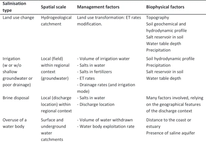
2.2.2. Human interventions causing soil and water salinisation ... 37
2.2.3. Water and soil salinisation damages to Ecosystems, Human health and Resources ... 40
2.2.4. Complexities related with salinisation in space and time... 40
2.3.CRITICAL ANALYSIS OF SALINISATION IMPACT ASSESSMENT METHODS IN LCA ... 42
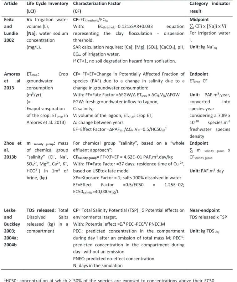
2.3.1. Salinisation associated with irrigation: Feitz and Lundie (2002) ... 42
2.3.2. Salinisation associated with overuse of a water body: Amores et al. (2013) ... 43
2.3.3. Salinisation associated with brine disposal: Zhou et al. (2013b) ... 44
2.3.4. Salinisation associated with salt release: Leske and Buckley (2003; 2004a; 2004b) ... 44
2.3.5. Lack of consistent frameworks ... 45
2.4.TOWARDS A CONSISTENT FRAMEWORK FOR SALINISATION IMPACTS ASSESSMENT IN LCA: METHODOLOGICAL ISSUES AND RECOMMENDATIONS ... 47
2.4.1. Context of LCIA for assessing salinisation impacts ... 47
2.4.2. Modelling options for the different salinisation types ... 47
2.4.3. Toward operationalisation ... 59
2.5.CONCLUSION ... 55
ACKNOWLEDGMENTS ... 56
REFERENCES CHAPTER 2... 57
CHAPTER 3 ... 66
INVENTORY OF FIELD WATER FLOWS FOR AGRI-FOOD LCA: CRITICAL REVIEW AND
RECOMMENDATIONS OF MODELLING OPTIONS
ABSTRACT ... 663.1.INTRODUCTION... 67
3.2.CRITICAL ANALYSIS OF WATER INVENTORY DATABASES ... 68
3.2.1. Water inventory and agri-food LCA databases ... 68
3.2.2. Limitations of water inventory and agri-food LCA databases ... 74
3.3.1. Model specifications description ... 77
3.3.2. Modelling approach selection ... 81
3.3.3. Further developments of models, tools and databases ... 85
3.4.CONCLUSION ... 86
ACRONYM LIST... 89
REFERENCES CHAPTER 3... 89
CHAPTER 4 ... 98
E.T.: AN OPERATIONAL FIELD WATER AND SALT FLOWS MODEL FOR AGRICULTURAL LCA
ILLUSTRATED ON CITRUS
ABSTRACT ... 984.1.INTRODUCTION... 99
4.2.MATERIAL AND METHOD: FIELD WATER AND SALT FLOWS MODEL PRESENTATION... 100
4.2.1. Model specifications and general principles ... 100
4.2.2. E.T. Model description ... 101
4.2.3. Validity domain of E.T. ... 108
4.2.4. Model testing ... 109
4.3.RESULTS AND DISCUSSION: MODEL TESTING ... 115
4.3.1. Comparison of E.T. outputs to other model formalisms ... 115
4.3.2. Sensitivity of E.T. model outputs to parameters’ variations ... 118
4.3.3. Testing of E.T. model for different scenarios of practice... 118
4.3.4. Model with degraded data ... 119
4.3.5. Model limitations and improvement perspectives ... 121
4.3.6. Model usage recommendations ... 123
4.3.7. Model outputs comparison with databases ... 123
4.3.8. Model usage within a LCA study ... 125
4.4.CONCLUSION ... 126
ACKNOWLEDGMENTS ... 127
REFERENCES CHAPTER 4... 127
CHAPTER 5 ...132
LIFE CYCLE ASSESSMENT OF A PERENNIAL CROP INCLUDING AN IN-DEPTH ASSESSMENT OF
WATER USE IMPACTS: THE CASE OF A MANDARIN IN MOROCCO
ABSTRACT ... 1325.1.INTRODUCTION... 133
5.2.MATERIALS AND METHODS ... 133
5.2.2. LCA goal and scope ... 134
5.2.3. Inventory of Moroccan mandarin production: from cradle-to-farm-gate ... 135
5.2.4. Life cycle impact and damage assessment ... 139
5.2.5.COMPARISON WITH PUBLISHED LCA STUDIES ON CITRUS... 142
5.3.RESULTS ... 142
5.3.1. Market gate - midpoint ... 142
5.3.2. Farm gate - midpoint ... 144
5.3.3. Farm gate - endpoint ... 147
5.4.DISCUSSION ... 148
5.4.1. Comparison with published references on citrus ... 148
5.4.2. Water - energy nexus ... 149
5.4.3. Water use impacts ... 150
5.4.4. Perspectives ... 154
5.5.CONCLUSION ... 157
ACKNOWLEDGEMENTS ... 158
REFERENCES CHAPTER 5... 158
DISCUSSION AND PERSPECTIVES (IN FRENCH)...164
COMMENT MIEUX EVALUER LES IMPACTS ASSOCIES AUX FLUX D’EAU ET DE SELS ? ... 164
COMMENT REALISER UN INVENTAIRE PERTINENT DES FLUX D’EAU ET DE SELS MOBILISES DANS LES SYSTEMES AGRICOLES ? ... 167
EST-IL POSSIBLE D’APPLIQUER LE MODELE D’INVENTAIRE DES FLUX D’EAU ET LES INDICATEURS ASSOCIES POUR EVALUER DES PRATIQUES AGRICOLES ? ... 169
GENERAL CONCLUSION (IN FRENCH) ...177
PUBLICATIONS LIST ...180
PEER-REVIEWED PUBLICATIONS ... 180
PRESENTATIONS IN CONFERENCES ... 180
PARTICIPATION IN BOOKS AND REPORTS ... 180
ANNEXES ...181
LCA OF LOCAL AND IMPORTED TOMATO: AN ENERGY AND WATER TRADE-OFF
Journal of Cleaner Production - DOI: 10.1016/j.jclepro.2014.10.007 ABSTRACT ... 1841.INTRODUCTION ... 185
2.MATERIALS AND METHODS ... 186
2.2. LCA goal and scope ... 187
2.3. Inventory of Moroccan tomato production: from cradle-to-farm-gate ... 187
2.4. Life cycle impact and damage assessment ... 189
2.5. LCA comparison of Moroccan and French off-season tomato production... 190
3.RESULTS AND DISCUSSION ... 190
3.1. Environmental impacts of the Moroccan off-season tomato production and delivery ... 190
3.2. LCA comparison of imported Moroccan and local French production systems ... 192
3.3. The need for a reliable inventory for accurately modelling the impacts of freshwater use ... 194
4.CONCLUSION ... 196
ACKNOWLEDGEMENTS ... 196
REFERENCES ... 197
TABLES AND FIGURES ... 201
LCA OF LOCAL AND IMPORTED TOMATO:AN ENERGY AND WATER TRADE-OFF -SUPPLEMENTARY INFORMATION ... 207
CHAPTER 1 - SUPPLEMENTARY INFORMATION - HOW TO ASSESS THE IMPACTS ASSOCIATED
WITH WATER USE IN AGRICULTURAL LCA? ...212
CHAPTER 2 - SUPPLEMENTARY INFORMATION - SALINISATION IMPACTS IN LIFE CYCLE
ASSESSMENT: A REVIEW OF CHALLENGES AND OPTIONS TOWARDS THEIR CONSISTENT
INTEGRATION ...224
CHAPTER 3 - SUPPLEMENTARY INFORMATION - INVENTORY OF FIELD WATER FLOWS FOR
AGRI-FOOD LCA: CRITICAL REVIEW AND RECOMMENDATIONS OF MODELLING OPTIONS ..232
CHAPTER 4 - SUPPLEMENTARY INFORMATION - E.T.: AN OPERATIONAL FIELD WATER AND
SALT FLOWS MODEL FOR AGRICULTURAL LCA ILLUSTRATED ON CITRUS ...238
CHAPTER 5 - SUPPLEMENTARY INFORMATION - LIFE CYCLE ASSESSMENT OF A PERENNIAL
CROP WITH IN-DEPTH ANALYSIS OF WATER USE IMPACTS: THE CASE OF A MANDARIN IN
MOROCCO ...243
GLOSSARY ...248
Table des figures
Figure 1. Schematic overview of risks associated with main agricultural production systems. (FAO Land & water (2011) - the state of the world's land and water resources for food and agriculture)... 3 Figure 2. LCA: A global method. On this figure, water footprint refers to the volumetric blue, green and grey
waters (Source: P. Roux - IRSTEA)... 4 Figure 3. Four steps of the LCA methodology with simplified substances inventory and impact categories: 1.
the goal and scope definition, 2. the inventory analysis, 3.the environmental impact assessment, and 4. the interpretation that should be performed at each of the three previous steps. Arrows between the different steps show that LCA is an iterative process... 5 Figure 4. Flow diagram of the cause and effect chain for aquatic eutrophication (ReCiPe method): from human
interventions to the midpoint impacts, and finally the endpoint damages on Ecosystem quality (based on ILCD Handbook (2011)) ... 6 Figure 5. Technosphere (agricultural system under study) and Ecosphere (environment receiving the
emissions) boundary depend on the soil status (dotted line). ... 7 Figure 6. From the inventory to midpoints and damages related to water in LCA. At the inventory level,
processes can use water and/or pollute water through the emission of substances. Impacts related to water use include the impact on the water resource and water pollution. Ultimately, these impacts damage the three areas of protection. ... 8 Figure 1.1. Water use impact modelling framework in LCA: 1. Product life cycle modelling including many
processes using and/or polluting water, 2. Inventory of water flows for each process in terms of volume and quality (inventory flows requirement depends on the method), 3. Environmental impact assessment: water footprint profile includes water deprivation impacts (based on scarcity or availability indicator), but also acidification, eutrophication, ecotoxicity and other impacts related to water degradation. Hatched boxes represent impacts not addressed in this review. ... 13 Figure 1.2. An overview of methods addressing water use in LCA with classification for the three areas of
protection. At midpoint, scarcity indicators (addressing only water quantity) are differentiated from availability indicators (addressing both water quantity and quality). *Hoekstra et al. (2012): not developed specifically for LCA but compatible... 14 Figure 1.3. Inventory schemes and characterization factors for Pfister et al. (2009, 2014) as water scarcity
indicator, and Boulay et al. (2011) as water availability indicator. ... 16 Figure 1.4. Cause-effect chains from the inventory to the areas of protection of human health, ecosystem
quality, and resources (adapted from Bayart et al. 2010 and Kounina et al. 2013). The pathways considering water quality degradation are emphasised in pink colour. One potential missing cause-effect chain from the framework described by Kounina and colleagues (2013) is the loss of water quality damaging the AoP Resource. ... 22 Figure 2.1. Human-driven salinisation environmental mechanisms and positioning of approaches proposed in
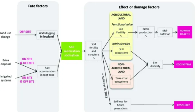
the literature. Long dash lines represent controversial pathways in the scientific community. ... 41 Figure 2.2. Soil salinisation impacts on Human Health, Ecosystems and Resource: fate and effect factors
positioning on the cause-effect chain and relations between agricultural and non-agricultural lands.51 Figure 2.3. Salinisation associated with irrigation and deposition of salts: technosphere and ecosphere
boundaries options and corresponding parameters to account for in the inventory or in the impact assessment. ... 52
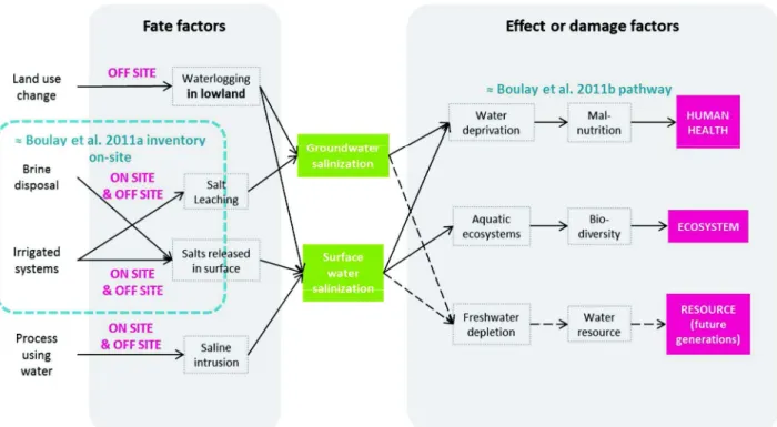
Figure 2.4. Water salinisation impacts on Human Health, Ecosystems and Resource: fate and effect factors positioning on the cause-effect chain and Boulay et al. inventory and damage to human health methods positioning. ... 54 Figure 3.1. The general scheme of recent water inventory and agri-food LCA databases (Water Database
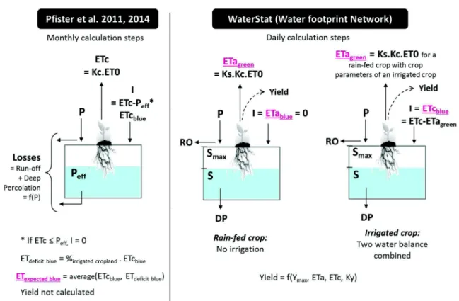
(Quantis), WFDB, Ecoinvent v3): calculations steps and main assumptions to determine the different water flows. Databases are based on a water balance: input water = output water. Each water flow is geolocalised at country or large watershed scale. ... 69 Figure 3.2. Scheme of the calculation methods used in water inventory databases (Pfister et al. (2011,
2014) and WaterStat). ... 71 Figure 3.3. Agri-food LCA databases and Quantis water database are using data from water inventory
databases for the water elementary flows of agricultural systems. Water inventory databases are using formalisms of water balance and crop evapotranspiration estimation from Allen et al. 1998 (also denoted as: FAO N°56). ... 71 Figure 3.4. Gradient of complexity and accuracy in the different possible approaches (databases and models)
for the inventory of field water flows, and associated type of LCA study. ... 82 Figure 4.1. The modular structure and main formalisms for the E.T. model. NRCS: Natural Resources
Conservation Services ... 101 Figure 4.2. Salt and water balances modules in the model, input data (orange), determining factors (green),
and interaction between the salt and water balances (double arrows). The evaporation-transpiration module is assessed through a dual approach: soil evaporation and plant evaporation-transpiration are assessed separately. ... 102 Figure 4.3. Potential evaporation and transpiration estimation methods: single and dual approaches are
presented according to their historical developments and corresponding references. The dual approach implemented in the model is framed by double red boxes. ... 106 Figure 4.4. Climate data for the case study Mandarin crop grown in Morocco: minimum relative humidity
(RHmin), average temperature, rainfall and reference evapotranspiration (ETo). In 2007, 2008, and 2011, assumptions were required to disaggregate monthly values or fill data gaps (details in Table 4.1). ... 109 Figure 4.5. Water flows estimated by the E.T model (E/T partitioning, water and salinity stresses) and other
model formalisms, expressed in m3 per ton of Mandarin over seven years (from planting in 2007 to 2015) ... 115 Figure 4.6. Actual evapotranspiration (ETa) estimated by the E.T model (E/T partitioning, water and salinity
stresses) and other model formalisms, expressed in mm.day-1, over seven years (from planting in 2007 to 2015) ... 115 Figure 4.7. Evolution over time of salts in soil water (red line) and salts in percolating water (blue line) (in
g.m-2) for the E.T. model (E/T partitioning, water and salinity stresses). ... 116 Figure 4.8. Actual transpiration (Ta) estimated with water stress or with water and salinity stresses, expressed
in mm.day-1, over seven years (from planting in 2007 to 2015) ... 117 Figure 4.9. Scenario analysis of the E.T. model. The input variables tested are: wz= wetted zone by the
irrigation, z= rooting depth, %G= percentage of ground covered by vegetation, CN= curve number (for the runoff calculation), Kcb= basal crop coefficient, ETo = reference evapotranspiration... 119 Figure 4.10. Values of crop coefficient Kc (continuous lines) and basal crop coefficient Kcb (dotted lines) for
citrus from the litterature and simulated by the E.T. model (dashed line). Year 2012/2013, 6 years-old orchard. no cc: no cover crop. ... 120
Figure 4.11. ETa blue [m3.ton-1] of small citrus provided by water inventory databases at country scale (WaterStat, Pfister et al. 2011 and 2014) and by the E.T. model for a Mandarin Nadorcott orchard located in South-West Morocco. ... 124 Figure 4.12. E.T. model integration within a LCA study: input and output water flows will be converted in
terms of impacts on the environment thanks to existing water impact assessment methods (e.g.: Pfister et al. (2009) and Boulay et al. (2011a, and b))... 126 Figure 5.1. Flow diagram for the Moroccan Mandarin production and delivery to the French market
(2007-2015, Bahira region, Morocco). ... 135 Figure 5.2. Representation of elementary water flows and associated characterisation factors of Pfister et al.’s
(2009) and Boulay et al.’s (2011a&b) methods: ... 140 Figure 5.3. Contribution analysis of 1kg of Moroccan Mandarin at French market gate. Midpoint impacts were
assessed with ReCiPe Midpoint (H) V1.12... 143 Figure 5.4. Contribution analysis of 1kg of Mandarin at farm gate in Morocco. Midpoint impacts were
assessed with ReCiPe Midpoint (H) V1.12... 145 Figure 5.5. Water deprivation impacts of 1kg of Mandarin at farm gate, calculated with the method from
Pfister et al. (2009) (water scarcity indicator), and two versions of the method from Boulay et al. (2011b) with and without considering the degradative use of the water (water availability and scarcity indicators). ... 147 Figure 5.6. Contribution analysis to endpoint damages of 1kg of Mandarin at farm gate in Morocco (ReCiPe
Endpoint (H) V1.12). Water consumption damages were assessed with Pfister et al. (2009). ... 147 Figure 5.7. Climate change, acidification, eutrophication impacts (calculated with CML (2001)), and
non-renewable energy (calculated with CED), from different LCA studies on citrus and for this study. Results are expressed per kg of fruit at farm-gate. Nota: no value available for non-renewable energy for Sanjuan et al. (2005). ... 149 Figure 5.8. Water inventory flows and water deprivation impacts of Mandarin cultivation (nursery not
included). Water inventory flows (in m3.ton-1) are estimated with E.T. model or from database, and water deprivation impacts (in m3eq.ton-1) associated with these water flows are calculated with different assessment methods. Results are expressed per tonne of export fruits (allocation included), even for databases. ... 152 Figure 5.9. Representation of elementary water flows and associated characterisation factors (CF) of Boulay et
al. (2011b) method when addressing the impacts from rainfall water consumptive and degradative use. Rainfall water, evapotranspiration from rainfall (∆ETa green), and rainfall water released in the environment through runoff (∆ROgreen) and deep percolation (∆DPgreen and ∆DPblue) should be quantified as the difference with the reference state. ... 154
Table des tableaux
Table 2.1. Key management and biophysical factors involved in secondary salinisation, per salinisation type. . 39
Table 2.2. Inventory requirement, characterization factors and category indicator results of salinisation impact assessment methods in LCA ... 46
Table 3.1. Sources of input data of the global crop water databases WaterStat and Pfister et al. (2011) ... 73
Table 3.2. Model specifications and data sources for the inventory of water flows for the LCA-based ecodesign of cropping systems. ... 79
Table 3.3. Required input variables for simulations with AquaCrop (Based on Vanuytrecht et al. (2014)) ... 85
Table 3.4. Database of modelling approaches for the assessment of water flows according to the objective of the Agri-food LCA study, the data available, the resources and time available ... 88
Table 4.1. Model input variables and parameters description, temporal resolution, determining factors, and average values for the case study (Mandarin in Morocco), and data sources and assumptions ... 110
Table 4.2. E.T. versus other model formalisms ... 113
Table 4.3. Basal crop coefficient values for citrus tested in the E.T. model ... 114
Table 4.4. Scenarios of practices tested in the E.T. model and corresponding values ... 114
Table 4.5. Percentage variations of water flows simulated with E.T. for the range values of initial conditions (S(i) and ECsoil water(i)) and for the average fraction of Total Available Water (TAW) that can be depleted from the root zone before water stress occurs (p). ... 118
Table 5.1. Agronomic data summary for the main orchard development phases: average yield, NPK fertilisation, irrigation volumes and energy, main active substances for plant protection ... 138
Table 5.2. Data sources for volume and quality of water elementary flows, and associated characterisation factors (CF) for Boulay et al. (2011,a&b) (water availability indicator) and Pfister et al. (2009) methods (water scarcity indicator). ... 141
Table 5.3. Cradle-to-farm-gate LCA results per kg of Mandarin for a selection of environmental indicators (Midpoint impacts assessment with ReCiPe Midpoint (H) V1.12) ... 146
Table 5.4. Cradle-to-farm-gate LCA results per kg of fruit for a selection of environmental indicators (ReCiPe Midpoint (H); Cumulative Energy Demand) for the Clementine and Mandarin grown in Morocco .. 155
Table 5.5. Nutrient application rates for the Mandarin grown in Morocco (this study) and published citrus LCA studies... 156
Structure of the thesis
A brief introduction will demonstrate the importance of analysing the environmental impacts of agricultural systems and the relevance of using the Life Cycle Assessment (LCA) methodology. Then, a bibliographical review will specifically address the assessment of water use impacts in chapter 1. Through the identification of general research needs, this review will introduce the scientific questions addressed in this dissertation and its specific objectives. Next, the core of the dissertation will be organised into four main chapters including 1/ a proposal of a framework for accounting for salinization impacts in LCA, 2/ a review of available models for field water and salt flows inventory in LCA, 3/ a description of a new model for estimating these fluxes and its implementation into a complete LCA case study for citrus in Morocco. In the last section, a general discussion (in French) will then be proposed before the conclusions:
2
Introduction
Why doing Life Cycle Assessment of agricultural systems?
1.1. Feeding the planet without destroying it
1.1.1. Agriculture is feeding the planet, but has many impacts on the environment
Agriculture fulfils a function of production: providing food for human, but agriculture activity can reduce the ability of ecosystems to provide goods and services (Tilman et al. 2002). The stake is to ensure the food provision without affecting -too much- the environment, in other words, it is to have a sustainable agriculture.
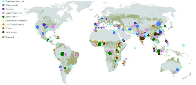
Agriculture - including crops, livestock, forest, fisheries and aquaculture- is the main human activity responsible for the use of land and water resources (FAO 2013), and has many impacts on the environment (Fig. 1). Agriculture has an impact on climate change, notably through the emissions of greenhouse gases: 50% of the methane emitted into the atmosphere by human activity is due to crop and livestock production alone (FAO 2013). Agriculture has an impact on water resources through its consumption and degradation: 70% of global water withdrawals are done by agriculture (World Water Assessment Program 2009) (and irrigated crops sustain 40% of the global food production (Abdullah 2006)), and the main source of nitrate and ammonia pollution in waters come from agriculture (FAO 2013). Indeed, since agriculture started, the cycle of different elements from the soil (N, C, P) has been altered which led to their partial decrease in soil and to their accumulation in the sediments from different ecosystems. The use of inputs such as pesticides and mineral fertilizers later on added more nutrients and more pollutants into motion on earth, thus exacerbating this dual phenomenon of soil fertility decrease and environmental compartments pollution. (Fert)irrigation water is a driver of pollutions because irrigation return-flows usually carry more nutrients, salts and pesticides than in source water, impacting downstream agricultural, natural systems (Tilman et al. 2002). Thus, agricultural activity contributes to water quality degradation and causes (eco)toxicity, eutrophication and acidification impacts.
1.1.2. An increasing pressure…
The pressure on agricultural systems is increasing because of the growing world population, the demand from other competing uses to food production (e.g. biofuels), and climate change (Mateo-sagasta and Burke 2010). Actually, climate change alone will have substantial impacts on the irrigation water demand, according to projections based on a set of seven global hydrological models (Wada et al. 2013). This increasing pressure is accentuated a vicious circle: impacts on the environment of agriculture have, in turn, negative impacts on agriculture production (FAO 2011).
3
Figure 1. Schematic overview of risks associated with main agricultural production systems. (FAO Land & water (2011) - the state of the world's land and water resources for food and agriculture)
1.1.3. Identify the environmental hot spots and mitigation options
There is a growing awareness of the importance of environmental impact of food products. European policies promote the quantification of the environmental performance of food supply chains (Peacock et al. 2011). Developing more sustainable and efficient production systems is crucial in a context where we have to produce more and pollute less. The stakes of the environmental assessment are thus considerable at a time when we are wondering how to feed the planet. This is a society issue affecting and involving politicians, farmers and consumers.
Life Cycle Assessment (LCA) is a suitable tool to evaluate the environmental impacts of the functions of agricultural systems, and a powerful decision-making tool for the different stakeholders.
1.2. LCA of agricultural systems: challenges
1.2.1. LCA methodology
LCA is a standardized and internationally recognized methodology to assess the environmental impacts of a function (product or service) over its entire life cycle (from cradle-to-grave) (ISO 2006a; ISO 2006b). Contrary to single indicator methodologies such as carbon footprint or water footprint, LCA is a multicriteria assessment method addressing a wide range of impact categories such as global warming potential, ecotoxicity, eutrophication, and acidification (Fig. 2).
4
Figure 2. LCA: A global method. On this figure, water footprint refers to the volumetric blue, green and grey waters (Source: P. Roux - IRSTEA)
Risk-Assessment (site-specific) and LCA (product-specific) are complementary approaches: a product can be analysed using LCA and, at the same time, a Risk Assessment can be performed for a number of core processes in the chain, in which the emphasis is on the local environmental impacts (Guinée et al. 2002). According to the ISO norm, LCA consists of 4 steps: the goal and scope definition, the inventory, the characterization of impacts and the interpretation. In practice, all the inputs and outputs (resources extraction and emissions to the environment) associated with the product system are inventoried in the inventory stage, then, each flow is converted in environmental impacts indicators thanks to characterization factors. These impacts (at midpoint level) can be further aggregated into damage indicators on Human health, Ecosystems quality and Resources (at endpoint level) (Fig. 3). Human health, Ecosystems quality and Resources are defined in LCA as the areas of protection: the entities that we want to protect. Nevertheless, their precise definition is not fully consensual since they depend on the vision of sustainability and the underlying values (Adams 2006; Dewulf et al. 2015). This is an interesting feature (and maybe a weakness point) of LCA: LCA aims to be science-based, but involves assumptions and value choices (Guinée et al. 2002). The importance is thus to make these choices transparent while reporting a LCA study.
The inventory and environmental impacts and damages are related to the studied function of the system through the functional unit (e.g: provide 1 kilogram of tomato on the French market).
LCA is a tool presenting many assets:
▪ its holistic approach addresses many environmental impacts, making visible possible transfers of
pollution between different technologies fulfilling the same function, and considers the whole life cycle of the product, allowing the identification of environmental hot spots,
▪ its functional approach allows for a more powerful eco-design regarding the service provided, ▪ its quantified characterisation of impacts is based on scientific modelling of environmental
mechanisms,
▪ it is based on an international consensus and a large community of experts and scientists, ▪ it is supported by operational tools and databases.
5
Figure 3. Four steps of the LCA methodology with simplified substances inventory and impact categories: 1. the goal and scope definition, 2. the inventory analysis, 3.the environmental impact assessment, and 4. the interpretation that should be performed at each of the three previous steps. Arrows between the different steps show that LCA is an iterative process.
1.2.2. The cause and effect chain or environmental “pathway”
Environmental mechanisms are complex and their modelling is a challenging task. One of the main challenges of LCA is to assess the global potential impacts of a given substance emission. The cause– effect chain is the cascade of environmental processes provoked by a substance emission (the cause), until the midpoint impacts (the effect), and finally the endpoint damages to the area of protection. Figure 4 gives an illustration of the cause-effect chain in LCA for the aquatic eutrophication potential. For a detailed and up-to-date presentation of the principles and practice of life cycle impact assessment, see Hauschild and Huijbregts (2015), part of the book series LCA Compendium: The Complete World of Life Cycle Assessment.
6
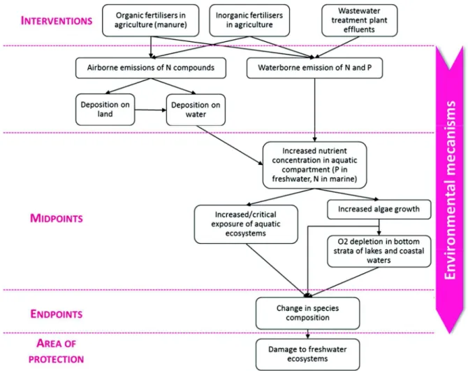
Figure 4. Flow diagram of the cause and effect chain for aquatic eutrophication (ReCiPe method): from human interventions to the midpoint impacts, and finally the endpoint damages on Ecosystem quality (based on ILCD Handbook (2011))
1.2.3. Why applying LCA to agricultural systems is relevant?
LCA is particularly relevant for the assessment of agricultural systems. Indeed, agriculture supply chains are globalised (Hubacek et al. 2014): imported food products rely on imported agricultural inputs such as fertilizers. LCA, through its global approach, account for all processes along the supply chains occurring all-over the world. Thus, agriculture is responsible for many impacts, at different localisations in the world, and there are impact categories for which the level of impact depends on the localisation of the emission. If global warming has a global effect on earth (the place of the greenhouse gas emission does not matter, and the impacts concern the whole planet), this is not the case for water eutrophication which is a local or regional impact (nitrate emissions will affect the local scale and the impacts will depend on the sensitivity of the environment)(Azevedo et al. 2013). Thus, we can distinguish three levels of spatial differentiation of impact assessment: site-generic, site-dependent, and site-specific assessments. Site-generic is globally valid (e.g. climate change), site-dependent operates on the regional scale, and site-specific is only locally applicable (Potting and Hauschild 2006).
Although LCA is relevant for evaluating agricultural systems, the methodology has to cope with complexities associated with agricultural systems:
7
1.2.4. The inventory: a crucial LCA stage for agricultural systems
In agricultural LCA, the objective is to relate the outputs to the inputs of the system accounting for the climate, the soil characteristics and the agricultural practices. Differentiating the practices for the inventory calculation is a major challenge because they are highly diverse and interact with soil and climate. Fluxes generated during agricultural processes are submitted to soil and climate influence and variability, but depend also on agricultural practices. It is therefore difficult to estimate field emissions such as nitrogen emissions due to fertilisation. Furthermore, it is crucial to define what is an emission, through the system delimitation. The definition of the temporal and physical (spatial) boundaries of the agricultural system (the technosphere) is complex because soil is both part of the agricultural system studied (the growing medium) and of the environment (Fig. 5)
Figure 5. Technosphere (agricultural system under study) and Ecosphere (environment receiving the emissions) boundary depend on the soil status (dotted line).
1.2.5. One limitation of LCA relates to the modelling of freshwater use impacts.
There are deficiencies in the impact assessment associates with water use.Water has a double status in LCA: it is an environmental compartment receiving pollutions, and a resource (Nota: the same is valid for the soil). Impacts on water as a compartment have received detailed attention over the last decades through the development of several environmental impacts (Eutrophication, Acidification, …) (see Finnveden et al. (2009) and Pennington et al. (2004) for a review), whereas the impact from water use has only recently been considered and has not already resulted in consensual methods. Both water use (consumptive and degradative use) and emissions of substances polluting water are impacting waters (Fig. 6).
8
Figure 6. From the inventory to midpoints and damages related to water in LCA. At the inventory level, processes can use water and/or pollute water through the emission of substances. Impacts related to water use include the impact on the water resource and water pollution. Ultimately, these impacts damage the three areas of protection.
1.3.2. The importance of scales
Although the demand for water has doubled since 1960 (Millennium Ecosystem Assessment 2005), human populations did not reach the critical “planetary boundary” for freshwater use according to Rockström et al. (2009). Planetary boundaries express the limits of human pressure the whole planet can endure without critical damage. But Rockström's study failed to address the pressure on the water resource by considering it as a global resource. In 2015, an update of the planetary boundaries proposed a new boundary: freshwater use at the river-basin scale (Steffen et al. 2015). But the definition of the riven-basin scale water boundary is limited by the hazardous estimation of environmental water flow requirement (water flow to preserve for the natural ecosystems).
This example is an illustration the importance of the scales when addressing water: if the global water volume remains constant at earth level over time, its potential scarcity is expressed at the local or regional scales, and at specific temporal scales depending on the contexts. Moreover, water is available at variable levels of quality which drive its possible functions and uses.
Both the expression of the water scarcity phenomenon at various non-global scales and the interaction between its qualitative and quantitative dimensions make extremely complex the modelling of water use impacts in LCA.
9
1.4. Conclusion
Identifying the environmental hot spots and mitigation options of agriculture are crucial tasks in a context where humanity has to produce more and pollute less. Life Cycle Assessment (LCA) is a powerful tool to evaluate the environmental impacts of agricultural systems, but this methodology is still fraught with shortcomings and research challenges. One limitation of LCA relates to the modelling of freshwater use impacts. This is particularly important when evaluating agricultural systems which are both consuming and degrading water.
Payen et al. (2015) (See annexes) showed that accounting for water use impacts (even with a perfectible method) can radically change the outcomes of a LCA study comparing the environmental impacts of locally-grown vs. imported tomato. But the study also showed that the assessment of freshwater use impacts and damages still has shortcomings, leading to an underestimation of the impact for the Moroccan tomato. Therefore, the framework for assessing the impacts of water use in LCA will be analysed in depth in a bibliographic review in the next chapter.
References Introduction
Abdullah K bin (2006) Use of water and land for food security and environmental sustainability. Irrig Drain 55:219–222. doi: 10.1002/ird.254
Adams WM (2006) The Future of Sustainability: Re-thinking Environment and Development in the Twenty-first Century. IUCN, The World Conservation Union,Zurich, Switzerland, 19pp.
Azevedo LB, Henderson AD, van Zelm R, et al. (2013) Assessing the importance of spatial variability versus model choices in Life Cycle Impact Assessment: the case of freshwater eutrophication in Europe. Environ Sci Technol 47:13565–70. doi: 10.1021/es403422a
Dewulf J, Benini L, Mancini L, et al. (2015) Rethinking the Area of Protection “Natural Resources” in Life Cycle Assessment. Environ Sci Technol 49:5310–5317. doi: 10.1021/acs.est.5b00734
FAO (2013) FAO Statistical Yearbook 2013 - World food and agriculture - Part 4: Sustainability dimensions. Food and Agriculture Organisation, Rome, Italy, 57pp
FAO (2011) The state of the world’s land and water resources for food and agriculture (SOLAW) - Managing systems at risk. Food and Agriculture Organization of the United Nations, Rome, Italy and Earthscan, London, UK, 308pp
Finnveden G, Hauschild MZ, Ekvall T, et al. (2009) Recent developments in Life Cycle Assessment. J Environ Manage 91:1–21. doi: 10.1016/j.jenvman.2009.06.018
Guinée J, Gorrée M, Heijungs R, et al. (2002) Life cycle assessment - An operational guide to the ISO standards. Leiden, The Netherlands
Hauschild MZ, Huijbregts MAJ (2015) Life Cycle Impact Assessment. Book series: LCA Compendium – The Complete World of Life Cycle Assessment, Springer.
10
Hubacek K, Feng K, Minx JC, et al. (2014) Teleconnecting Consumption to Environmental Impacts at Multiple Spatial Scales. J Ind Ecol 18:7–9. doi: 10.1111/jiec.12082
ISO (2006a) ISO 14044: Environmental Management - Life Cycle Assessment Requirements and Guidelines. ISO, Geneva, Switzerland
ISO (2006b) ISO 14040: Environmental Management - Life Cycle Assessment Principles and Framework. ISO, Geneva, Switzerland
Mateo-sagasta J, Burke J (2010) SOLAW Background Thematic Report - TR08 Agriculture and water quality interactions: a global overview. FAO, Rome, Italy, 46pp
Millennium Ecosystem Assessment (2005) Ecosystems and human well-being: synthesis. Island Pre, Washington, DC, 155pp
Payen S, Basset-mens C, Perret S (2015) LCA of local and imported tomato : an energy and water trade-off. J Clean Prod 87:139–148. doi: 10.1016/j.jclepro.2014.10.007
Peacock N, De Camillis C, Pennington D, et al. (2011) Towards a harmonised framework methodology for the environmental assessment of food and drink products. Int J Life Cycle Assess 16:189–197. doi: 10.1007/s11367-011-0250-5
Pennington DW, Potting J, Finnveden G, et al. (2004) Life cycle assessment Part 2: Current impact assessment practice. Environ Int 30:721–739. doi: 10.1016/j.envint.2003.12.009
Potting J, Hauschild M (2006) Spatial Differentiation in Life Cycle Impact Assessment: A decade of method development to increase the environmental realism of LCIA. Int J Life Cycle Assess 11:11– 13. doi: 10.1065/lca2006.04.005
Rockström J, Steffen W, Noone K, et al. (2009) A safe operating space for humanity. Nature 461:472– 475. doi: 10.1038/461472a
Steffen W, Richardson K, Rockstrom J, et al. (2015) Planetary boundaries: Guiding human development on a changing planet. Science (80- ) 347:1259855–1259855. doi: 10.1126/science.1259855
Tilman D, Cassman KG, Matson P a, et al. (2002) Agricultural sustainability and intensive production practices. Nature 418:671–7. doi: 10.1038/nature01014
Wada Y, Wisser D, Eisner S, et al. (2013) Multimodel projections and uncertainties of irrigation water demand under climate change. Geophys Res Lett 40:4626–4632. doi: 10.1002/grl.50686
World Water Assessment Program (2009) The United Nations World Water Development Report 3: Water in a Changing World. The United Nations Educational, Scientificand Cultural Organization (UNESCO), Paris, France, and Earthscan, London, United Kingdom.
11
Introduction showed that LCA is a powerful but perfectible tool for evaluating the environmental impact of agricultural systems. Chapter 1 further investigates the strengths and limitations of LCA regarding the assessment of water use impacts.
12
Chapter 1
How to assess the impacts associated with water use in agricultural LCA?
This chapter provides a synoptic literature review on the methods used in Life Cycle Assessment (LCA) for addressing water use impacts, emphasising the main differences, strengths and limitations of the methods through the successive steps of inventory, midpoint and endpoint impact assessment. The objective is to identify the research needs toward accurate LCA of agricultural products.
1.1. Water footprints terminologies
It is paramount to clarify the terms, in accordance with the terminology promoted and used in the ISO (International Organization for Standardization) standards and in recent publications from the UNEP (United Nations Environment Programme) – Setac (Society of Environmental Toxicology and Chemistry) working group Water Use in LCA (WULCA) (e.g.: Boulay et al. 2015a; Boulay et al. 2015b; Boulay et al. 2015c). First, volumetric footprint must be distinguished from impact-oriented water1 footprint. From an
LCA perspective, the volumetric accounting of water use (m3) is not sufficient because numerically
smaller footprint can cause larger impacts depending on the context (Berger and Finkbeiner 2010). The ISO standard on Water Footprint (ISO 14046 2014) provides a definition of water footprint: “the metric(s) that quantifies the potential environmental impacts related to water”. This impact-oriented water footprint is different from previous work on volumetric water footprint of a product or a nation from Allan (1998), Hoekstra and Hung (2002), defined as the sum of blue, green and grey water footprints. The water footprints terminologies can be confusing, especially because LCA researchers mobilised the existing concepts of blue, green and grey waters to name the water inventory flows in LCA. However, the recent ISO 14046 standard does not use these “colour” but refers to the hydrological nature of water flows. It defines actual water types as: groundwater, surface water, brackish water, seawater, fossil water and precipitation in relation to the water cycle and hydrological mechanisms. A comprehensive water footprint assessment “considers all environmentally relevant attributes or aspects of natural environment, human health and resources related to water, including water availability and water degradation (negative change in water quality)” (ISO 14046 2014, 3.3.3).A water footprint profile should therefore illustrate the double status of water: because it includes impacts related to water degradation such as aquatic eutrophication or aquatic ecotoxicity, considering water as a living compartment, and also includes impacts related to water use, such as water deprivation, considering water as a resource. In practice though, two types of impact categories related to water use exist: water scarcity, refering to a consumptive use, and water availability, referring to a consumptive and degradative use. Indeed, water quality can also influence availability (ISO 14046 2014, 3.3.16). Thus, scarcity refers to the pressure on water resource from a quantity perspective only, whereas availability refers to the pressure on water resource due to both water quality degradation and quantity depletion
13
(Fig. 1.1). To sum up, a complete water footprint profile should address both the effects of water quantity and quality change on the environment, for the resource-water and living compartment-water viewpoint (Fig. 1.1). The stake of a water footprint assessment is to convert volumes of water used and/or degraded by a product or service, into potential environmental impacts: from the inventory to the impacts and damages.
In this review, we will only present the methods used to assess the impacts on the water as a resource and not on the water as a compartment (e.g. eutrophication) (hatched boxes in Fig. 1.1).
Figure 1.1. Water use impact modelling framework in LCA: 1. Product life cycle modelling including many processes using and/or polluting water, 2. Inventory of water flows for each process in terms of volume and quality (inventory flows requirement depends on the method), 3. Environmental impact assessment: water footprint profile includes water deprivation impacts (based on scarcity or availability indicator), but also acidification, eutrophication, ecotoxicity and other impacts related to water degradation. Hatched boxes represent impacts not addressed in this review.
1.2. An overview of the different methods
If LCA was an adolescent, water use impact analysis in LCA would be a baby. But a fast growing baby: over the last 6 years, life cycle impact assessment of water use has evolved rapidly with many new methods emerging (Tendall et al. 2013). Several reviews of these methods exist: Berger and Finkbeiner (2010), Jeswani and Azapagic (2011), Berger and Finkbeiner (2012), Kounina et al. (2013), Boulay et al.
14
(2015c). This chapter is based on these reviews, the original publications they are referring to, but also more recent publications.
The general framework of water use impact modelling in LCA includes: description of the product life cycle in terms of processes using water, inventory of water flows of all processes throughout the product life cycle, environmental assessment either at midpoint level through the conversion into water deprivation impacts by multiplying with characterisation factors, or at endpoint level (also called damage assessment) on the three Areas of Protection (AoP) (Fig. 1.1). Nevertheless, water use impact assessment methods are addressing different cause-effect chains and rely on different water use inventory schemes and characterisation models (Kounina et al. 2013). There are midpoint and/or endpoint oriented (Fig. 1.2). To date, no single method allows for a comprehensive impact assessment of all possible impacts due to water use. Midpoint category indicators are either scarcity (e.g. Pfister et al. 2009) or availability indicators (e.g. Boulay et al. 2011), specific to one AoP (Mila i Canals et al. 2008) or covering all AoP (e.g. Pfister et al. 2009). Across all available methods, endpoint category indicators addressing the same AoP are neither identical, nor complementary. Thus, to obtain a comprehensive water footprint profile, the compilation of several methods would be required.
Figure 1.2. An overview of methods addressing water use in LCA with classification for the three areas of protection. At midpoint, scarcity indicators (addressing only water quantity) are differentiated from availability indicators (addressing both water quantity and quality). *Hoekstra et al. (2012): not developed specifically for LCA but compatible.
15
A complete list and description of methods addressing the impacts and damages of water use in life cycle impact assessment is provided in the supplementary information. The scientific bases and specificities of each method will be further presented and discussed in sections 1.3 (inventory), 1.4. (midpoint impact assessment) and 1.5. (endpoint impact assessment), the main discrimination criteria being whether the method accounts for water quality alteration or not.
1.3. Inventory schemes: water quantity, quality and source
1.3.1. The inventory scheme depends on the impact assessment method
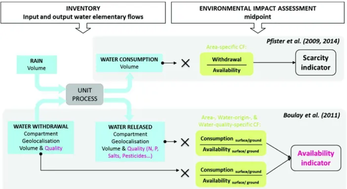
The ISO 14046 specifies that the inventory of water elementary flows shall include inputs and outputs from each unit process being part of the system to be studied, while respecting a balance. Information on each water elementary flow should include quantity, source, quality, form of water use, geographical location, and temporal aspects. But in practice, the water inventory requirements differ amongst methods. On the one hand, there are methods whose inventory is based solely upon the water consumed (Hospido et al. 2012; Milà i Canals et al. 2008; Pfister et al. 2009). Water consumption is water removed from, but not returned to, the same drainage basin (e.g.: evaporation, transpiration, integration into a product). Berger and Finkbeiner (2012) pointed that the continental evaporation recycling rate is important in some areas and advocated to account for evaporative water returned to the basin (via precipitation) in his method (Berger et al. 2014). On the other hand, there are methods relying on the water withdrawal (removal of water from any water body, permanently or temporarily) and the water released (returned to the same catchment area where it was withdrawn during the same period of time) like Boulay et al. (2011a, b) (Fig. 1.3). Indeed, a method accounting for water quality degradation cannot rely on the single water consumption flow since the quality of the withdrawn and released water flows have to be compared. The recommendations for LCA practitioners and researchers are to inventory both withdrawn and released waters (Bayart et al. 2010; Kounina et al. 2013).
Rainwater has a special and complex status because it relates both to land use and water use in the water cycle: this water flow is only accessible though the soil and for plants (except in the case of rainwater harvesting). The consumption of rainwater stored in the soil profile has received poor attention in LCA because it is considered less environmentally relevant from a pure water consumption perspective (Núñez et al. 2013). Most methods consider that the use of rainwater does not have direct effect on water scarcity/availability. Yet, soil water consumption has an influence on water availability in rivers and aquifers. Only Milà i Canals et al. (2008) and Núñez et al. (2013) proposed a method to account for rainwater use through the land-use effects on the water cycle. In Nuñez et al. (2013), the inventory flow is the net change in soil-water availability under the production system compared to the natural reference situation. But this approach has to cope with two issues: first, the definition of the potential natural vegetation and its water consumption, second, the fact that natural vegetation always consumes more water than an agricultural production system, thus leading to positive impact of the production system on the water availability. This shows the complexity to account for the water hydrological cycle and water flow redistribution within the LCA framework.
16
A detailed list of inventory requirements for each method is provided in the supplementary information.
1.3.2. The water sources must be distinguished as they might face different
scarcities/availabilities
In theory, “the inventory flows represent a set of water types each representing an elementary flow with its own characterisation factors” (Bayart et al. 2010). Indeed, each water type (source of water in the environment) has different renewability rates and functionalities. For example, differentiating groundwater from surface water in CF calculation is important because some regions suffer much more from groundwater scarcity and others more from surface water scarcity. Such a distinction is not made in Pfister’s method where surface and ground waters are weighted with a unique CF. Only a few methods differentiate water sources (except fossil water): Hospido et al. (2012) and Boulay et al. (2011a & b). Hospido and colleagues (2012) proposed to associate a specific CF for each water type of the irrigation profile: surface, ground, desalinated and non-conventional water (based on Milà i Canals et al. 2008 method). However, in practice, they allocate the same CF for surface and ground waters, and do not consider the water that may be released to the environment. Boulay et al. (2011a) not only proposed an inventory distinguishing the water sources, but also accounted for the quality of input and output waters through water categories.
Figure 1.3. Inventory schemes and characterization factors for Pfister et al. (2009, 2014) as water scarcity indicator, and Boulay et al. (2011) as water availability indicator.
17
1.3.3. Water quality has to be inventoried as quality degradation may contribute to water
deprivation
The WULCA group recommended the “use [of] water quality parameters to characterize freshwater flows”. Boulay and colleagues (2011a) developed an inventory method whereby water quality is related to a function assessing to which users the waters withdrawn and released are functional (useful) (Bayart et al. 2010). This functionality-based water inventory considers that water quality degradation can lead to water deprivation if not suitable anymore for specific users (Boulay et al. 2011a). Thus, it allows for an impact assessment associated with water quality consumption and degradation.
1.4. Midpoint impact assessment: water scarcity or availability?
At midpoint, most methods are characterizing a water deprivation impact, in cubic meter equivalent, i.e. a volumetric use is adjusted against the water scarcity/availability conditions that prevail at the place of consumption or withdrawal.
1.4.1. Water indices are used as characterisation factors
The Characterisation Factors (CF) used to convert the water inventory flows into impacts are based on water indices and represent the actual pressure on water resources. These water indices are originally non-LCA-based indicators and are recognized as proxies for water scarcity/availability (see supplementary information). They consist of a ratio of water use by different sectors to the water available, but vary depending on what is considered as “water use” (numerator) and water available (denominator). Indeed, they are either based on a withdrawal-to-availability ratio (Milà i Canals et al. 2008; Pfister et al. 2009; Ridoutt and Pfister 2010) or a consumption-to-availability ratio (Boulay et al. 2011b; Hoekstra et al. 2012). The CFs rely on existing water availability data from hydrological models at global scale such as WaterGAP or UNH/GRDC (Alcamo et al. 2003; Fekete et al. 2002). An alternative of global hydrological model was recently tested, using a large-scale hydrological modelling with the Soil Water Assessment Tool (SWAT)(Neitsch et al. 2009) (Scherer et al. 2015). This attempt showed that although the SWAT model outperformed the global models at large watershed scale, its use on a global scale is unlikely because of the high calibration efforts required (Scherer et al. 2015).
The related CF for each approach is then multiplied with the inventory elementary flows of water consumption (Milà i Canals et al. 2008; Pfister et al. 2009) or water withdrawal and release (Boulay et al. 2011b) (Fig. 1.3). See supplementary information for a detailed description of characterisation factors and the original water indices they rely on.
18
1.4.2. Water scarcity indicators vs. water availability indicators
To date, only the Water Impact Index (Bayart et al. 2014) and Boulay et al.’s (2011b) indicators are water availability indicators (i.e. considering that both water quantity and quality contribute to water deprivation). However, they do not model the same impact pathway since Bayart’s method assesses the effect of a change in quality based on environmental standards for ambient water, whereas Boulay’s method assesses the effect of a change in quality based on the functionality of water for human users (Boulay et al. 2015c). Bayart’s method is ecosystem-oriented and based on a distance-to-target approach (acceptable water pollution level), whereas Boulay’s method is human-oriented (functionality of water for human uses).
Since water quality degradation also contributes to water availability (ISO 14046 2014), the split between water quality & quantity for other methods such as Pfister et al. (2009) and Berger et al. (2014) is questionable. For example, Pfister et al. (2009) consider that a quality alteration do not affect water deprivation. This viewpoint divergence is important since Boulay et al. (2015c) demonstrated that calculating midpoint indicators based either on scarcity or on availability can greatly influence the results.
1.4.3. Open questions on characterisation factors
Regarding the CF’s
numerator,
should scarcity be a function of water withdrawal or water consumption? (i.e.: a consumption-to-availability (CTA) or a withdrawal-to-availability (WTA) ratio?). Boulay et al. (2011b) and Berger and Finkbeiner (2012) support the use of a CTA ratio because the use of WTA tends to overestimate the water scarcity as it includes the non-consumptive use of water (e.g. cooling water, return flow from irrigation use). Moreover, the CTA ratio ensures consistency between the inventory and the impact assessment, as water consumption is multiplied by a CF also based on consumption (Kounina et al. 2013). Conversely, Pfister and colleagues support the use of a WTA. Since the water quality is not accounted for in the inventory, they are indirectly compensating it through the impact assessment: the water index is indirectly considering the water degraded in the numerator because water withdrawal includes water that may be released in the environment in a degraded state. On the contrary, Boulay et al. (2011b) clearly assess both quantity and quality in the inventory: the volume of input and output flows are multiplied with a CTA ratio specific to the water source and category (reflecting the quality) (Fig. 1.3). Payen et al. (2015) (see annexes) illustrated another issue related to CFs: when the activity under study represents a significant part of water usage in the watershed/country, its contribution to the total water consumption/withdrawal is not marginal anymore. This means that the product is directly affecting the CF which should ideally account for this significant contribution.Regarding the CF’s denominator: What is the available amount of renewable water? Most indicators only consider renewable groundwater recharge and surface runoff (Alcamo et al. 2003; Döll and Fiedler 2008) and neglect ground and surface water stocks (Berger and Finkbeiner 2012). Berger and colleagues filled this gap in their new indicator accounting for these water stocks (Berger et al. 2014). As already
19
explained, the method from Boulay et al. (2011b) also filled this gap but in a more relevant way: not only the ground and surface water stocks are accounted for in the CF’s denominator, but surface and ground waters are also distinguished, each one having a specific characterisation factor, thus representing that different water sources have different availabilities.
1.4.4. Spatial and temporal scales: consistency with the goal and scope of the study
To convert the inventory into environmental impacts, it is necessary to consider the context of the studied system (the hydrological context, the water use competition…). The spatial resolution of the data (water scarcity indicators) and results (impacts) can be either at country, catchment or sub-catchment levels. Boulay et al. (2015c) showed that the scale at which the scarcity indicator is calculated significantly influences the indicators. Loubet et al. (2013) developed an indicator at the sub-catchment level to better account for the cascading effects that occur downstream of consumption in sub-basins, thus accounting for the location of water consumption within the basin. This spatial resolution allows considering that using water close to the outlet is less impacting (deprive less downstream users) than using water upstream at its source. Nevertheless, the question of the optimal scale remains (Boulay et al. 2015c).Regarding the temporal scale, most water scarcity indicators are calculated at the annual scale, which seems not relevant for regions with contrasted dry and humid seasons, and more particularly for agricultural water use (Tendall et al. 2013). However, Pfister and Bayer (2014) and Hoekstra et al. (2012) developed monthly scarcity indicators. The relevant temporal scale depends on the goal and scope of the study, the studied system, and its location.
1.4.5. Water indices versus fate and effect modelling
The use of scarcity/availability indices in LCA is still debatable because the link between water scarcity, water deprivation (midpoint) and damages on the AoP still has to be demonstrated (Kounina et al. 2013). Indeed, water scarcity indices are not referring to any actual environmental mechanism such as the water cycle and the actual effect on human health and ecosystems. A few methods do not use the water indices for impact assessment but adopt a two-step modelling approach: first analysing the fate of the water flow, and second its resulting effects on the environment. Such an approach is compliant with the thorough impacts assessment scheme for an emission: fate, exposure, and effect modelling. The methods based on this framework are all endpoint-oriented: they address the effects of water use on the Ecosystems, splitting the CF in a Fate Factor (FF) and an Effect Factor (EF) (e.g. Amores et al. 2013; Verones et al. 2013a; Verones et al. 2013b; van Zelm et al. 2011). The fate factor could be considered as a midpoint indicator, but they are not comparable with one another (e.g.: wetland area change (Verones et al. 2013a), salt concentration change in the wetland (Amores et al. 2013)). Indeed, these methods are designed to provide endpoint indicators, the midpoint being only an intermediate in the assessment. But they present the advantage of describing the environmental mechanisms of the water use, contrary to the water index approaches. For example, Verones et al. (2013a, 2013b) addressed the damages of