HAL Id: hal-01392292
https://hal.archives-ouvertes.fr/hal-01392292
Submitted on 26 Jun 2020
HAL is a multi-disciplinary open access
archive for the deposit and dissemination of
sci-entific research documents, whether they are
pub-lished or not. The documents may come from
teaching and research institutions in France or
abroad, or from public or private research centers.
L’archive ouverte pluridisciplinaire HAL, est
destinée au dépôt et à la diffusion de documents
scientifiques de niveau recherche, publiés ou non,
émanant des établissements d’enseignement et de
recherche français ou étrangers, des laboratoires
publics ou privés.
Corinna Roy, Giovanni Occhipinti, Lapo Boschi, Jean-Philippe Molinié, Mark
A. Wieczorek
To cite this version:
Corinna Roy, Giovanni Occhipinti, Lapo Boschi, Jean-Philippe Molinié, Mark A. Wieczorek. Effect
of ray and speed perturbations on ionospheric tomography by over-the-horizon radar: A new method.
Journal of Geophysical Research Space Physics, American Geophysical Union/Wiley, 2014, 119 (9),
pp.7841-7857. �10.1002/2014JA020137�. �hal-01392292�
RESEARCH ARTICLE
10.1002/2014JA020137
Key Points:
• A new 3-D ionospheric tomography method for monostatic OTH radar • The raypath deflection effect is
not negligible
• Three-dimensional reconstruction of the electron density over Europe is possible
Correspondence to:
C. Roy, roy@ipgp.fr
Citation:
Roy, C., G. Occhipinti, L. Boschi, J.-P. Molinié, and M. Wieczorek (2014), Effect of ray and speed pertur-bations on ionospheric tomog-raphy by over-the-horizon radar: A new method, J. Geophys. Res. Space Physics, 119, 7841–7857, doi:10.1002/2014JA020137.
Received 28 APR 2014 Accepted 18 AUG 2014
Accepted article online 22 AUG 2014 Published online 17 SEP 2014 Corrected 6 FEB 2015
This article was corrected on 6 FEB 2015. See the end of the full text for details.
Effect of ray and speed perturbations on ionospheric
tomography by over-the-horizon radar:
A new method
Corinna Roy1,2, Giovanni Occhipinti1, Lapo Boschi3, Jean-Philippe Molinié2, and Mark Wieczorek1
1Institut de Physique du Globe de Paris, Université Paris Diderot, Paris, France,2Office National d’études et de recherches
aérospatiales, Palaiseau, France,3Laboratoire iSTeP, Université Pierre et Marie Curie, Paris, France
Abstract
Most recent methods in ionospheric tomography are based on the inversion of the total electron content measured by ground-based GPS receivers. As a consequence of the high frequency of the GPS signal and the absence of horizontal raypaths, the electron density structure is mainly reconstructed in the F2 region (300 km), where the ionosphere reaches the maximum of ionization, and is not sensitive to the lower ionospheric structure. We propose here a new tomographic method of the lower ionosphere, based on the full inversion of over-the-horizon (OTH) radar data. Previous studies using OTH radar for ionospheric tomography inverted only the leading edge echo curve of backscatter ionograms. The major advantage of our methodology is taking into account, numerically and jointly, the effect that the electron density perturbations induce not only in the speed of electromagnetic waves but also on the raypath geometry. This last point is extremely critical for OTH radar inversions as the emitted signal propagates through the ionosphere between a fixed starting point (the radar) and an unknown end point on the Earth surface where the signal is backscattered. We detail our ionospheric tomography method with the aid of benchmark tests. Having proved the necessity to take into account both effects simultaneously, we apply our method to real data. This is the first time that the effect of the raypath deflection has been quantified and that the ionospheric plasma density has been estimated over the entirety of Europe with an OTH radar.1. Introduction
Most recent methods in ionospheric tomography are based on the inversion of the total electron content (TEC) derived from dual-frequency receivers of the Global Navigation Satellites System (GNSS), mainly the American Global Positioning System (GPS). The TEC is the integral of electron density along the raypath between the satellite and the receiver, computed from the phase difference between two signals emitted by the GPS satellite and measured at the receiver [Mannucci et al., 1993]. TEC is usually visualized as global or regional two-dimensional maps to show the state of the ionosphere [Mannucci et al., 1998]. The measure-ment of TEC on the raypath between satellites and receivers, jointly with some a priori information about the background ionospheric model, allows additionally to estimate the local electron density of the ionosphere using the inverse problem theory, [e.g., Tarantola, 2005].
GNSS ionospheric tomography was first tested in simulations by Austen et al. [1988], showing that numeri-cal tomography techniques can be used to produce two-dimensional vertinumeri-cal cross sections of the electron density in the ionosphere. Andreeva et al. [1990] published the first experimental result using TEC data collected at three receivers in Russia and reconstructed a two-dimensional vertical cross section of the ionosphere by satellite radio tomography for the first time.
The installation of global (e.g., the International GNSS Service) and regional (e.g., GNSS Earth Observation Network (GEONET) in Japan) ground-based GPS networks greatly increased the amount of available data and raypath coverage, making three-dimensional reconstruction of the ionosphere with time evolution (3-D + 1) possible. Since then, GPS-based computerized ionospheric tomography has been widely used to investigate the temporal and spatial variations of ionospheric structures [Hansen et al., 1997; Hajj et al., 1994;
Hernández-Pajares et al., 1998; Bust et al., 2004; Garcia et al., 2005; Ma et al., 2005; Yizengaw et al., 2005; Wen et al., 2007].
Although GPS is a powerful tool for studying the ionosphere, theoretical limitations of ionospheric tomog-raphy using GNSS satellite-to-Earth configuration have been discussed in detail in the literature [Yeh and
Raymund, 1991; Na and Sutton, 1994]. Apart from the spatial and temporal limitations associated with the
experimental arrangements, the data sets are often incomplete because of the finite sampling interval and the limited angle of view of each receiver. Additionally, most of the tomographic methods make the assumption of an invariant ionosphere during the time of measurement.
Notwithstanding those previous limitations, the major problems of ionospheric tomography using GPS are the following. First, the absence of horizontal raypaths, resulting in a low vertical resolution. Second, the high frequency of the GPS signal limits the sensitivity of the electromagnetic waves to the maximum of electron density in the ionosphere, nominally the F region at around 300 km altitude.
To overcome the major limitations of low vertical resolution, three approaches are possible. The first approach is to incorporate, in the reconstruction, extra information from other instruments, for instance ionosonde data, which allow for the determination of electron density in the lower ionospheric layers, such as the E (∼100 km) and F1 region (∼250 km). Heaton et al. [1995] tested the incorporation of scaled ionograms into the imaging and found improvement in the vertical profiles. Kersley et al. [1993] showed promising results with the incorporation of ionosonde data into the reconstruction algorithm and better agreement with the EISCAT (European Incoherent Scatter Scientific Association) measurements in the vicin-ity of the layer maximum. Markkanen et al. [1995] applied a Bayesian approach to simulated results and incorporated peak heights as a priori information in the reconstruction algorithm for calculating the F region electron density, which are compared with the EISCAT radar observations.
The second approach is to use general knowledge of the shape of ionospheric profiles to constrain the reconstruction results and to fill the information gap: The most widely used solution is the one proposed by Fremouw et al. [1992], who used a set of vertical orthonormal functions, created from ionospheric mod-els, to model the vertical profile. Unfortunately, existing ionospheric models are partially incorrect, because they fail to predict the strong day-to-day variations, consequently the reconstructions constrained with ver-tical profiles from ionospheric models are often inaccurate. Consequently, Fehmers et al. [1998] proposed a model-independent algorithm that compensates for the lack of horizontal raypaths with information that is not related to some specific model: basically, they impose that the electron density cannot be negative at high and low altitudes and is additionally smooth and vertically stratified. Their tests show moderate success with an error in the layer-height estimation on the order of 90 km.
Another recently developed method uses occultation data. The technique is based on using the radio sig-nals continuously broadcast by the GNSS satellites (GPS/Global Navigation Satellite System/Galileo) that are measured by a receiver on a low Earth orbit satellite. Along its way through the ionosphere the signal has been refracted due to free electrons that modify the refraction index. Since both satellites move over time, this technique allows a vertical scanning of successive layers of the atmosphere. Rius et al. [1997] showed that the combined measurement of GPS TEC by ground stations and occultations improved the vertical resolution. Additionally, the authors proved that the use of ground stations alone is insufficient for vertical reconstruction of the electron density.
To deal with the instabilities of the solution, introduced by noise and the ill conditioning of the problem, different reconstruction algorithm have been tested for ionospheric tomography. Several works [Kersley et al., 1993; Heaton et al., 1995; Mitchell et al., 1995; Pryse et al., 1995; Vasicek and Kronschnabl, 1995] applied the iterative multiplicative algebraic reconstruction technique [Gordon et al., 1970] that attempts to minimize the difference between measured and calculated TEC values by modifying the background iono-sphere until the differences are acceptably small. Kunitsyn et al. [1994a, 1994b] tried an iterative algebraic reconstruction technique algorithm that incorporates some prior information into each pixel in the iono-spheric grid that they wish to solve. The solution obtained with this algorithm, however, is severely limited because it is very sensitive to the initial ionospheric model. To cope with this problem, Wen et al. [2010] recently proposed the constrained algebraic reconstruction technique, where cells not hit by any ray extract information from neighbor cells.
The purpose of our work is to present a new tomographic method of the lower ionosphere (≤300 km) based on the full inversion of over-the-horizon (OTH) radar data. Our method can integrate easily GPS TEC obser-vations of ground-based or onboard receivers (occultation), as well as ionosonde measurements when such data are available.
Figure 1. Schematic representation of our parametrization ofjrays with elevation angle𝜑andicells with the raypath deflection induced by a local-ized perturbation (e.g., gray cell) producing a perturbed ray (red) compared to the unperturbed ray (black).
OTH radar takes advantage of the refraction properties of the iono-sphere, where the presence of free electrons causes the electromag-netic (EM) wave deflection in the ionosphere. Consequently, the emit-ted signal, after deflection in the ionosphere, can reach the ground beyond the horizon, typically up to thousands of kilometers away from the transmitter. There, the signal is backscattered and goes back to the receiver following the same ray-path (Figure 1). The received signal contains all information about the propagating medium. We empha-size that the point where the signal is backscattered is not fixed and changes with the ionization of the propagating medium.
Previous studies in ionospheric tomography by OTH radar are all based on the inversion of the leading edge echo curve, which contains, for each frequency, only the information of the ray with minimal group delay (measured from the emitter to a point of first contact with the Earth). To estimate the three major ionospheric parameters (the critical frequency fc, the peak height, and the semithickness for each layer), two approaches to solve the inverse problem are possible. Either fitting the observed leading edge with a quasi-parabolic ionospheric layer [Rao, 1974; Bertel and Cole, 1988; Ruelle and Landeau, 1994; Landeau et al., 1997]; or using ray tracing to numerically simulate the leading edge [Coleman, 1998; Fridman and Fridman, 1994; Fridman, 1998].
A major drawback of using only the leading edge is that valuable information present in the data is neglected. To overcome this limitation, we set up an inverse problem taking into account the complete radar data set. We use the ray-tracing tool TDR (Tracé de Rayon) [Occhipinti, 2006] to calculate the synthetic prop-agation time. This code traces rays in an a priori heterogenic 3-D ionospheric model NeQuick [Radicella and
Leitinger, 2001] and in the elliptical WGS84 coordinate system [National Imagery and Mapping Agency, 2000],
solving numerically the Eikonal equation, describing the propagation of rays in a medium, by a fourth-order Runge-Kutta method. It neglects the Earth’s magnetic field, in order to apply the method to all OTH radars that are not able to determine the wave polarization and consequently cannot discriminate between the ordinary and extraordinary mode, induced by the geomagnetic field. In section 4, the calculated propaga-tion time is compared with the propagapropaga-tion time measured by the OTH radar. In our inverse problem, the electron density in the ionosphere is directly estimated from the difference between the calculated and measured propagation time (section 4 and Figure 10).
As a consequence of the measurement characteristics and geometry of OTH radar, the major challenge of this methodology is imposed by the measurement geometry. EM waves emitted by OTH radars are reflected in the ionosphere then arrive at the ground where they are backscattered to the receiver following the same raypath. Though we treat only the monostatic case in this work, the method could be easily generalized to bistatic cases, where the receiver and emitter are not at the same location.
We present here a new ionospheric tomography method that takes into account, jointly, the velocity varia-tion of electromagnetic waves induced by the electron density variavaria-tion, as well as the induced perturbavaria-tion in the raypath (section 2). The developed methodology will be tested using a set of synthetic bench-mark tests (section 3) and will be applied to real data from the OTH radar Nostradamus (New Transhorizon Decametric System Applying Studio Methods) [Bazin et al., 2006] in section 4.
2. Theory
2.1. The Forward Problem
The propagation of high-frequency (HF) radio waves in the ionosphere can be described using ray theory. Assuming an isotropic ionospheric medium, neglecting the Earth magnetic field
6 8 10 12 14 16 10 15 20 25 30 35 40 45 50 55 60 Frequency (MHz) Elevation (degree) prop. time (ms) 0 1 2 3 4 5 6 7 8 6 8 10 12 14 16 10 15 20 25 30 35 40 45 50 55 60 Frequency (MHz) prop. time lin. (ms)
0 1 2 3 4 5 6 7 8 6 8 10 12 14 16 10 15 20 25 30 35 40 45 50 55 60 Frequency (MHz) dT (%) 0.5 1 1.5 2 2.5 3
Figure 2. (left) Propagation time calculated without approximation (first line of equation (3)) versus (middle) linearized
propagation time (calculated with the second line of equation (3)), and the (right) difference between them in percent. Computation for 1071 rays traced with elevation angle10◦–60◦and frequency 6–16 MHz.
and losses in the ionosphere, the propagation time along the raypath s(n(⃗r))is given by Fermat’s principle:
Tphase=
1
c∫s(n)
n(⃗r)ds, (1)
where c is the speed of light, n(⃗r)the refractive index of the medium, and⃗r position.
Assuming the ionosphere is a stationary, isotropic, and horizontal stratified medium, the unmagnetized refractive index depends only on the frequency feof the emitted EM wave and the electron density Ne(⃗r),
n(⃗r)= √ 1 − e 2N e ( ⃗r) 4π2𝜖 0mefe2 ≈ √ 1 −80.6Ne ( ⃗r) f2 e , (2)
where𝜖0is the vacuum permittivity and e and meare the charge and the mass of the electron, respectively. The layered structure of the ionosphere produces a change of the refractive index as a function of altitude and bends EM waves emitted at high frequency (HF) toward the ground to locations beyond the horizon, typically up to thousands of kilometers away from the transmitter. By replacing the refractive index (2) in equation (1) and linearizing by a first-order Taylor series expansion, the propagation time of an EM wave can be separated into two parts:
Tphase= 1 c∫s(n) √ 1 −80.6Ne ( ⃗r) f2 e ds ≈ 1 c∫s(n) ds −40.3 cf2 e ∫s(n) Ne(⃗r)ds, (3) where the first integral of the second line describes the propagation in the vacuum and the second one the delay introduced by the ionosphere. Figure 2 shows the limit of the linearization comparing the first and second line of equation (3). The difference between the exact and linearized propagation time is always smaller than 3.5% when elevation angle is less than 60◦.
Equation (3) allows to calculate, using the ray-tracing code TDR described by Occhipinti [2006], the propa-gation time Tphasesynthof any EM wave with a given frequency fein any given ionospheric model with electron
density N0 e(⃗r). Tphasesynth= 1 c∫s(n) ds −40.3 cf2 e ∫s(n) N0 e ( ⃗r) ds.
We introduce an electron density perturbation𝛿Ne(⃗r)of the a priori model Ne0(⃗r) to describe the real
ionosphere Ne0(⃗r) + 𝛿N
e(⃗r). Then the propagation time in the real ionosphere is given by
Treal phase= 1 c∫s(n) ds −40.3 cf2 e ∫s(n) ( N0 e ( ⃗r)+𝛿Ne(⃗r))ds = Tphasesynth−40.3 cf2 e ∫s(n) 𝛿Ne ( ⃗r)ds.
We then obtain a travel time perturbation𝛿Tphasethat is the difference between propagation times in the
real ionosphere and in the a priori model (e.g., Figure 10):
𝛿Tphase= Tphasereal − T synth phase= − 40.3 cf2 e ∫s(n) 𝛿Ne ( ⃗r)ds (4)
This solution allows us to compute the travel time perturbation𝛿Tphaseas a function of an electron density
perturbation𝛿Neof the a priori model Ne0. The difference between the propagation time measured by the
OTH radar and the one computed by TDR is directly linked to the electron density perturbation𝛿Ne.
We emphasize that this approach is based on the hypothesis that the raypath s(n) in the real ionosphere and in the a priori model is the same. That means that we are supposing that the electron density variation𝛿Ne
only introduces variations in the speed of the EM waves and not in the raypath. Consequently, we call this approach the v method.
2.2. The Inverse Problem
In order to solve numerically our problem, we choose a parametrization of N homogeneous, nonoverlap-ping blocks, indexed i, where the electron density perturbation𝛿Ne(⃗r) can be expressed as
𝛿Ne ( ⃗r)= N ∑ i = 1 𝛿mi⋅ Bi ( ⃗r), (5)
where the electron density perturbation in the block i is𝛿miand N known basis functions Bi(⃗r) are
Bi ( ⃗r)= { 1 if⃗r in block i, 0 otherwise
Consequently, equation (4) for the jth measurement of travel time perturbation takes the following form:
𝛿Tj= − 40.3 f2 ejc N ∑ i = 1 𝛿midsij. (6)
where dsijis the length of raypath segments within block i of ray j.
Introducing the matrix A of size M × N, where M is the number of travel time measurements and N is the number of basis functions (i.e., the number of blocks in the parametrization of our ionospheric model), equation (6) can be rewritten as
𝛿Tj= N
∑
i = 1
𝛿miAji. (7)
In tensor notation equation (7) takes the form
𝛿T = A ⋅ 𝛿m, (8)
where𝛿m is the vector of model parameters with N unknown electron density perturbations 𝛿mi,
matrix containing the M × N raypath segments dsijof the jth ray in block ith, as well as the ray coefficient, Aji= − 40.3 f2 ejc dsij.
2.3. Solution of the Inverse Problem Regularization
Following Menke [1989] we solve equation (8) seeking the model that minimizes the L2norm for both data
and model, namely, ∥𝛿T − A ⋅ 𝛿m ∥2= min and ∥𝛿m ∥2= min. The first condition imposes the best fit to the
data, and the second condition minimizes the discrepancy from the a priori model. These two conditions are equivalent to solving the following two equations:
𝛿m =(AT⋅ A)−1⋅ AT⋅ 𝛿T ⇔ ∥ 𝛿T − A ⋅ 𝛿m ∥2= min
𝛿m = AT⋅(A⋅ AT)−1⋅ 𝛿T ⇔ ∥𝛿m ∥2= min
It is known that inverse problems in geophysics generally present a number N of parameters (here the vector𝛿m) larger than the number M of observations (here the vector 𝛿T). Consequently, the problem is underdetermined, and the matrices AT ⋅ A and A ⋅ ATcannot be inverted. The matrices are close to
singu-lar, and even if the inverse matrices formally exist, they are often ill conditioned; that is, small changes in the data vector (𝛿T) lead to large changes in the model estimation (𝛿m).
To find a more stable solution (𝛿m) balancing the sensitivity to the data, as well as the coherence with the a priori model, Menke [1989] suggests the following damped least squares solution
𝛿m =(AT⋅ A + 𝜆 ⋅ I)−1⋅ AT⋅ 𝛿T, (9) which minimizes the cost function ∥𝛿T − A ⋅ 𝛿m ∥2+𝜆 ∥ 𝛿m ∥2, where𝜆 is a regularization parameter and I
the identity matrix.
It is not possible to minimize both terms simultaneously, but the parameter𝜆 controls the emphasis that we put on the conflicting requirements. In the section 3.2, we highlight the way how to select the best value of
𝜆 satisfying our problem.
2.4. Taking the Raypath Deflection Into Account
In monostatic OTH radars, the end points of the rays (where the signal is backscattered by the ground) are not known. Consequently, the location of the scattering point can change for a constant elevation angle and depends on the electron density variation𝛿Ne(⃗r) in the ionosphere (Figure 1). As a result, the raypath
deviation, introduced by the variation of the scattering point, can introduce an additional shift𝛿Tphaseray in the propagation time. We extend the theory described above, in order to take into account jointly not only the speed variation (v method) but also the raypath deflection induced by the variation of the scattering point, what we call the v & r method. Snieder and Spencer [1993] showed that both effects can be combined in the perturbation approach, and the two effects are simply additive to first order. Based on equation (31a) of
Snieder and Spencer [1993] we can write the total observed time delay as 𝛿Tphase= − 40.3 cf2 e ∫s(n) 𝛿Ne ( ⃗r)ds +𝛿Tphaseray . (10)
If s(n) is the raypath in the a priori model N0
e(⃗r) and s∗(n) is the raypath in the perturbed model N0e(⃗r)+𝛿Ne(⃗r),
𝛿Tray phaseis described by 𝛿Tray phase= 1 c∫s∗(n) ds∗−1 c∫s(n) ds +40.3 cf2 e [ ∫s(n) N0e(⃗r)ds − ∫s∗(n) N0e(⃗r)ds∗ + ∫s(n)𝛿Ne (⃗r)ds − ∫s∗(n)𝛿Ne (⃗r)ds∗ ] . (11)
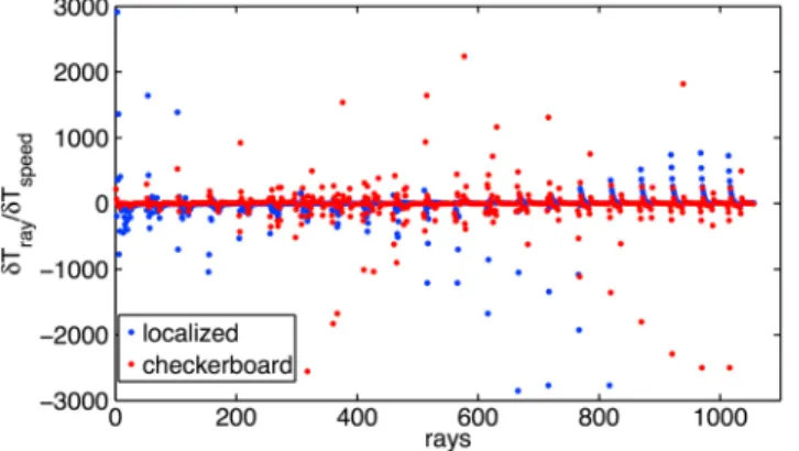
Figure 3 compares the values of𝛿Tphasevelocityand𝛿Tphaseray for a selected set of rays and shows that the raypath deflection is not negligible. This is discussed in more detail in section 3.1.
Figure 3. The ratio of𝛿Tray(equation (11)) to𝛿Tspeed(equation (4)) com-puted for the localized perturbation (Figure 4) and checkerboard (Figure 5) target models. The number of raypath are arranged in such a way that for one frequency (6–16 MHz), the elevation angle has been varied between 10◦and60◦. The peaks correspond to low elevation angles between 10◦ and 30◦for each frequency.
In this section, we extend the the-ory described above, in order to take into account jointly, not only the speed variation (v method) but also the raypath deflection induced by the variation of the scattering point (v & r method).
𝛿Tray
phasedepends on𝛿Ne, since raypath
deflections are caused by electron density perturbations. To set up an inverse problem, allowing us to deter-mine𝛿Nebased on observations of
𝛿Tphase, we therefore write𝛿Tphaseas
a linear function of𝛿Ne. The study of
Snieder and Spencer [1993] also
indi-cates that sensitivity kernels k(⃗r) can be defined such that
𝛿Tray
phase= ∫
s(n)
k(⃗r) ⋅ 𝛿Ne(⃗r) (12) where k(⃗r) is the data kernel [Menke, 1989], which in the v method described above is just a delta function along the unperturbed ray s(n). Here the kernel contains the Fréchet derivatives𝜕T∕𝜕m, where 𝜕T is a per-turbation in the propagation time caused by a perper-turbation in the model m. If the relation between the model m and the propagation time T is linear, the sensitivity function k(⃗r) can be computed numerically. In practice, using the parametrization described above, we impose a localized electron density perturbation of arbitrary amplitude𝛿Ne∗
i at only the ith cell; consequently, we can compute by ray tracing the partial time
perturbation𝛿T∗
j along the jth ray induced by𝛿Ne
∗
i in the ith cell:
𝛿T∗
j = kij⋅ 𝛿Ne∗i. (13)
This allows us to create our base function
kji= 𝛿T∗ j 𝛿Ne∗ i ,
that, following our linear hypothesis, is valid for a general case. We emphasize for additional clarity that the perturbed propagation time𝛿T∗
j is computed following equation (11), where the perturbed raypath
s∗(n) is traced in the a priori model plus the perturbation𝛿Ne∗
i only in the ith cell. We can finally express
equation (10) as 𝛿Tj= − 40.3 f2 ejc N ∑ i = 1 𝛿midsij+ N ∑ i = 1 kji𝛿mi, (14) or, in a tensor formalism as
𝛿T = (A + A′
)⋅ 𝛿m, (15)
where A′ij= kij. The general inverse method solution described in the section 2.3 is applied to the matrix A in the case of v method, and to the matrix A + A′in the case of v & r method.
3. Inversion Results for Synthetics
In order to validate and compare the two methods described in the previous sections, we generate synthetic data by the ray-tracing TDR in a known a priori ionospheric model, NeQuick [Radicella and Leitinger, 2001] that we call Nea priori, plus an additional perturbation that we call𝛿Netarget. The𝛿T is calculated as a difference
of propagation time in Nea priori+𝛿Netargetminus the propagation time in Nea priori. We emphasize that the
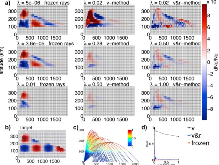
Figure 4. (a) Inversion results for the localized electron density perturbation benchmark with three different methods and for three different values of𝜆. Inver-sions for the best regularization parameter𝜆best(middle row) for each method: frozen rays (left column),vmethod (middle column), and v & r method (right column). (b) Target model. (c) Ratio between plasma frequency and emission frequency along the raypath quantifying the sensitivity of each ray to the propagat-ing medium. Rays are most sensitive to the medium where the ratio is approximately 1. (d)Lcurves for the frozen rays,vmethod, and v & r method. Diamonds correspond to the best values of regularization𝜆, i.e.,5.62 ⋅ 10−5, 0.2, and 0.63 respectively.
Additionally, we compute the vector of travel time perturbations𝛿Tfrozensatisfying exactly the hypothesis
that the electron density perturbation𝛿Netargetmodifies only the speed of EM waves (equation (4)); rays are
frozen in the a priori model configuration. This data set represents the idealized case of no raypath
perturba-tion, as if the ray end points were known; we shall invert it to separate the effects of poor data coverage and unknown raypath deflection or model resolution.
Independent of the method used (v or v & r), as well as for the synthetic data set (𝛿T or 𝛿Tfrozen), the solution
of our inverse problem𝛿m has to correspond to 𝛿Netarget. We emphasize that all synthetic data are
com-puted numerically by TDR in electron density continuous models (Na priorie and𝛿N
target
e ) and not in discretized
models following our parametrization. This is equivalent to introduce a noise in the synthetics in the order of 12%. The target model𝛿Ntargete is parametrized using the above described parametrization for comparison
with the solution𝛿m.
Quantitatively, we simulate rays with elevation angles between 10◦and 60◦and in the frequency range 6–16 MHz, as this is the operating capacity of the Nostradamus OTH radar [Bazin et al., 2006]. The back-ground ionosphere Nea prioriwas generated for October at 12:00 UT with a solar flux of 198.1 solar flux units.
Figure 5. Same as Figure 4 but for a checkerboard perturbation. Diamonds of theLcurves correspond to the best values of regularization𝜆, i.e.,3.6 ⋅ 10−5, 0.28,
and 0.5, respectively, for the frozen ray,vmethod, and v & r method.
covering an area of 2500 km in distance and reaching up to 400 km altitude. Each pixel of the grid has a dimension of 25 km in distance and 20 km in altitude. We traced here 1071 rays, using𝛿𝜙 = 1◦in the elevation angle and𝛿f = 0.5 MHz for the emission frequency, in accord with the capability of the radar Nostradamus.
We apply here the described methods to two different𝛿Netarget. The first is an ionospheric perturbation of a
localized electron density perturbation of 0.1% of the background model Nea priori(Figure 4), and the second
is a checkerboard perturbation with the same order of amplitude (Figure 5). In the next section we comment in detail on the results of our synthetic tests.
The synthetic data set inverted in this section includes ∼103rays. Ray tracing for the entire synthetic data
set in parallel on eight processors takes around 2 min on a grid with spatial resolution of 25 × 20 km and 2000 cells. The 2-D inversion result for the v method is obtained after 5 min for the first iteration. The per-formance of the v & r method is grid dependent, because of the number of cells to perturb. For a grid with spatial resolution of 25 × 20 km and ∼103rays, it takes around 40 min. For comparison with GPS ionospheric
tomography we note that Seemala et al. [2014] can construct the 3-D electron density over Japan within 55 min on a grid with spatial resolution of 1◦in latitude/longitude using data of 748 GEONET stations. Reducing the horizontal resolution of their grid to 2◦, they obtain a 3-D image within 15 min.
3.1. The v Method Versus v & r Method
The inversion results for𝛿m of our first test are summarized in Figure 4, where the solutions obtained with the v method and the v & r method are directly compared with the idealized frozen rays solution
Figure 6.Lcurves for different𝜆ranges indicated in the top left for the (a) localized and the (b) checkerboard benchmark test using the v & r method for inver-sion. (c and d) Corresponding error curves for the explored range of regularization parameters. The red point represents the minimum error, and the red line is the sum over the target models, i.e.,∑cellsi = 1(dNe
Ne
)2
i. The errors converge to the red line when the solution is totally damped.
(subsection 3). Figure 4a shows the results for three different regularization parameters𝜆 where the inver-sion results for the best regularization parameter (section 3.2) are shown in the middle of each column. The best𝜆 is obtained by performing the inversion changing the regularization parameter and plotting the data misfit against the model misfit (i.e., L curve). The best regularization parameter lies at the maxi-mum curvature of this curve, as this represents a compromise between small misfit and small solution norm (section 3.2).
As a consequence of the strong variation of the ionospheric background (electron density equal to zero at around 80 km, and of the order of 1011− 1012e∕m3at around 300 km) and the emission frequency
depen-dence of the refraction index, EM waves emitted by the radar are particularly sensitive to the zone where the rays are reflected, where the plasma frequency fpis approximately equal to the emission frequency fe
(Figure 5c). This defines the area of good coverage (independent of inversion method), as illustrated by Figure 5c with comparison with the frozen-ray inversion.
As is to be expected, solution models depend significantly on the regularization parameter. This effect is less severe in the idealized frozen-ray case that resembles GPS ionospheric tomography (both end points of the ray are known). As soon as raypath deflections (end point perturbations) are taken into account in our syn-thetic data, the resolution deteriorates and the choice of𝜆 (equation (9)) affects more profoundly our results. The correct location (500 km distance, 200 km altitude) of the maximum anomaly in the target model is only reconstructed by the v & r method provided that an adequate value is assigned to𝜆. Furthermore, the
vmethod identifies a high dNe/Ne anomaly in the general area of 200–500 km in horizontal distance and 100–200 km in altitude but slightly mislocates it and does not reproduce its shape. The better performance of the v & r method compared to v method is confirmed by Figure 4d, where the v & r L curve [Tikhonov, 1963] has a more pronounced corner than the L curve obtained with the v method.
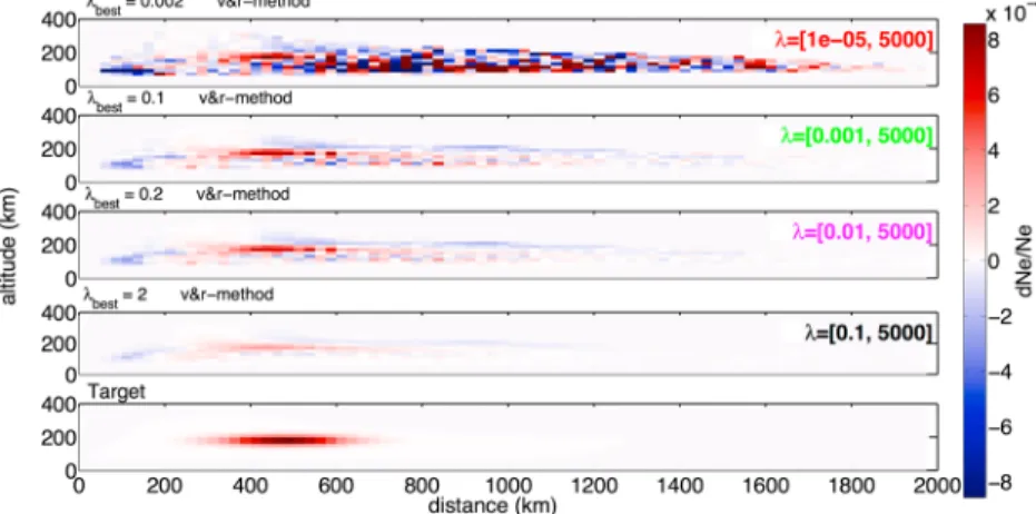
Figure 7. Inversion results using the v & r method with the best value of regularization chosen from theLcurves in Figure 6a for the localized perturbation in order to explore the sensitivity to the𝜆range. The bottom row shows the target model.
Compared to the result obtained with the ideal frozen rays, both the v and v & r methods occasionally intro-duce large-scale low dNe/Ne anomalies that do not correspond to any feature of the target model, where the sign of perturbation is always positive. We ascribe these artifacts to the nonlinear effects of raypath deflections, which (end points not being fixed) can in principle result in a faster propagation time even if the velocity perturbation is negative.
The inferences made from Figure 4 are confirmed by results illustrated in Figure 5, where the same set of inversions is conducted after replacing the target model (and associated synthetic data) with a checker-board. General comparison from Figures 4a and 5a, with Figures 4c and 5c, clearly show that the model is mainly reproduced in the zone of sensitivity where the emission frequency feis close to the plasma
frequency fp. This clearly emphasize the role of the coverage in our solution.
The selection of the value of𝜆 in order to choose the best solution is detailed in the next section. The following discussions are only applied to the v & r method.
3.2. Solution Dependence on Regularization
To quantify the robustness of our solutions obtained with both the v and v & r methods, we explore their dependence on our choice of regularization parameter𝜆. This analysis is limited to the synthetic data discussed in section 3.1 so that obtained solution can be compared to a target model.
We first observe that while the L curve method (Figures 4d and 5d) is useful to monitor qualitatively the trade-off between data misfit and model quality, it is not guaranteed to provide the “best” solution, i.e., the one closest to the real world. This is confirmed by Figures 6a and 6b, where we show how the choice of model-norm normalization results in a different curvature of the L-curve and thus a different choice of preferred model. Each plot of Figures 7 and 8 illustrates the result for𝜆bestobtained from the corresponding
Lcurve in Figures 6a and 6b. Figures 6c and 6d show the discrepancy between solution and target model for the same set of inversions and confirms that the model quality can be significantly affected by a inadequate choice of𝜆. Inspection of Figures 6c and 6d allows to identify the value of 𝜆 corresponding to the minimum error (discrepancy between solution and target model).
The corresponding𝜆bestare 0.63 and 0.5, respectively, and the inversion results corresponding to these
regularization parameters are shown in Figures 4 and 5 in the middle of the right columns. The differ-ence between target and model is less than 40% for the localized and less than 57% for the checkerboard perturbation, using the v & r method.
3.3. Iterative Approach
Since the results presented before are obtained after only one inversion, we attempt to improve the solu-tion by iterating the synthetic inverse problem. That means that the solusolu-tion models𝛿m found in section 3.1 can be used as starting models of new inversions. Raypaths are traced, the tomography matrix accordingly recomputed, and the differences between observed (or, in the present case, synthetic) and computed (in the new model) travel times replace the data to be inverted. In the interest of computational speed, we do
Figure 8. Inversion results using the v & r method with the best value of regularization chosen from theLcurves in Figure 6b for a checkerboard perturbation in order to explore the sensitivity to the𝜆range. The bottom row shows the target model.
not conduct a separate L curve analysis (which would involve several inversions) at each iteration, but we fix𝜆 to the trace of AT ⋅ A divided by 10 (v method) or the trace of (A + A′) divided by 100 (v & r method)
[Press et al., 1992, chapter 18]. These values were determined with a few preliminary test to properly tune convergence speed. The trace of the matrix is equal to the sum of eigenvalues and allows for a quick estima-tion of the eigenvalues that are well determined. Based on the them, the regularizaestima-tion can be adjusted. The inspection of eigenvalues of the matrices showed that the𝜆 selected by the L curve is to large in the case of the v method and too small for the v & r method compared to the largest eigenvalues. In the first case this is imposing large restriction to the solution, in the second case it is adding too much noise to the solution. The results of this exercise are summarized in Figure 9. The difference between target and solution is less than 30% for the v & r at iteration 13 and less than 40% for the v method at iteration 5. Nevertheless, after a critical number of iterations, the discrepancy between solution and target model starts growing for both the v and v & r inversions. We interpret this as an effect of the mentioned trade-off between velocity heterogeneity and raypath deflection (section 3.1). Entries of the tomography matrix can be either nega-tive or posinega-tive. Any given observation can be explained by a combination of both neganega-tive and posinega-tive
Figure 9. Data misfit∑raysj = 1(dT
T
)
jand model misfit as function of the number of iterations for the (top)vmethod and the (bottom) v & r method. The inversion results for the minimum (red point) of the model misfit (iteration 5 forvmethod and iteration 13 for v & r method) are shown on the right column.
Figure 10. Propagation time of the real data and synthetic data simulated by ray tracing as (a) function of frequency and
elevation angle, and the (b) difference (%).
heterogeneity whose amplitude might grow indefinitely as further iterations are performed. This problem is similar to that of selecting𝜆, and we suggest that the synthetic tests presented here can serve to deter-mine adequate values for such parameters, to be used in real inversions with the same data coverage. This approach rests on the assumption that the effect of limitations in data coverage is more important to model resolution than that of data noise.
4. OTH Radar Nostradamus and Real Data Inversion
In the following section we apply the developed v & r method to real data of the OTH radar Nostradamus exploring the regularization parameter range with a𝜆min = 10−3in accord with the results of the previous
Figure 11. Inversion of real data collected 14 March 2006, at 18:55 UT with azimuth 247◦, and for two different grids: (left) pixel size 50×20 km and (right) pixel size 25×20 km in distance and altitude. The middle row shows the result for the best regularization parameter𝜆best.
Figure 12. Vertical profiles of electron density at (a) 500 km distance and (b) 1000 km distance from the radar. The red
line shows the ionospheric a priori model NeQuick, and the black line is the solution obtained by the v & r method (the a priori model plus the perturbation).
synthetic tests. Nostradamus is a monostatic radar that consists of 288 biconical antenna elements dis-tributed over the arms of a three-branch star. The choice of this antenna arrangement allows beam forming with a coverage of 360◦in azimuth and elevation control with a resolution of approximately 2.35◦in azimuth and 5.43◦in elevation for a frequency of 11 MHz. The central part of the array (96 antennas) is dedicated to transmission and reception, and the entire array is used for reception allowing a greater capability in receiving beam forming. The Nostradamus configuration allows to investigate a very large area of more than thousands of kilometer in range all around Europe.
We use here data that were collected on 14 March 2006, at 18:55 UT, for a frequency range 6–16 MHz and scanning in elevation from 10◦to 60◦. We traced rays with frequency and elevation angle corresponding to
Figure 13. Electron density perturbation obtained by real data inversion measured by the OTH radar Nostradamus the
14 March 2006, at 18:55 UT in four azimuth directions, nominally67◦,157◦,247◦, and337◦.
the radar measurements in the a priori ionospheric model NeQuick given for this day and time. Figure 10 shows the comparison between data and the synthetics used to compute the vector𝛿T of travel time per-turbations for an azimuth of 247◦. The difference is around 30% for rays with low frequency of 7–9 MHz, and around 20% for the highest frequencies of 16 MHz.
Figure 11 shows an example of the inversion of the real data in one selected azimuth (247◦) for different values of regularization for the v & r method for two different grid sizes, i.e., (50 × 20 km and 25 × 20 km dis-tance and altitude). There is no significant difference in the inversion results for this range of parameters, and the resolved perturbation is mainly located at 200 km altitude with a maximum of 50%. It is not sur-prising that the perturbation is located around 200 km altitude, since at this time (18:55 UT) the E layer has nearly disappeared and only the F layer remains strongly visible. The v & r method shows stable results for all regularization parameters, validating the reliability of the solution.
To further explore the inversion results, we calculated vertical profiles of electron density from the inversion with the best regularization parameter for two different distances from the radar (500 km and 1000 km), and we compare them with the electron density from the a priori model NeQuick. The resulting vertical profiles (Figure 12) show a sensitivity to variations located between 120 km and 260 km of altitude in accord with the sensitivity of the EM waves emitted by the radar. Indeed, the plasma frequency below 120 km altitude is too small to affect the emitted signal, and the maximum altitude of reflection is located around 260 km. The recovered electron density perturbation is of the order of 10%.
In order to show the potential applications of the OTH radar Nostradamus in ionospheric tomography, we inverted here the data for the same day and time measured for different azimuths: 67◦, 157◦, and 337◦. The obtained tomographic images are plotted in Figure 13 over Europe, in the corresponding azimuthal directions. The electron density perturbation observed at 247◦azimuth at 200 km altitude is visible in all azimuthal directions.
We highlight that the developed methodology could easily include other kinds of ionospheric data, in particular TEC measurements by ground-located or onboard GPS receivers. Consequently, we note the possibility of creating regional and/or global ionospheric tomography based on joint inversions of various ionospheric monitoring data.
5. Conclusions
We developed a new linear ionospheric tomography method for over-the-horizon radar (OTH) that takes into account not only the effect of the electron density perturbation on the velocity of electromagnetic waves (v method) but also the effect on the raypath deflection (v & r method). The characteristic uncer-tainty of end points of the raypath followed by EM waves emitted by OTH radar makes this second effect comparable to the first. Based on synthetic tests, we showed the necessity of taking into account the ray-path deflection for tomographic inversions of the ionosphere. This is the first time that this problem is explored and emphasized in the OTH radar ionospheric tomography. Notwithstanding the methodological advance, the quality of the solution depends on the ray coverage, as well as, on the sensitivity of the rays to the medium that is the zone where the plasma frequency is close to the emission frequency of the propa-gating signal. This zone is strongly reduced at night, where only the high-frequency rays are reflected. The difference between target and solution for the localized perturbation is about 40% and 59% for the v & r and v methods, respectively, but can be reduced to 30% and 40% with iterations. For comparison we note that Seemala et al. [2014] archived a difference between target and solution of less than 10% with their GPS tomography over Japan during night.
Since the problem is underdetermined, meaning that the number of parameters to estimate is larger than the number of observations, our inversions have to be regularized. In order to find the best regularization parameter𝜆, we calculate a trade-off curve that quantifies the conflicting requirements between satisfying the data and the coherence with the a priori model. We highlight that the best regularization parameter
𝜆bestis strongly dependent of the explored𝜆 range. Consequently, we define a synthetic protocol to
deter-mine the𝜆 range to explore, in order to minimize the solution error. The selected 𝜆 range can be applied to real data inversion in order to maximize the quality of the solution.
Application of the developed methodology on real data gives stable solutions, showing the quality of the inversion method and the reliability of the solution. A 3-D ionospheric tomography over Europe, based on the inversion of the OTH radar Nostradamus data, has been presented here in order to show the potential application of the developed method. Although our method has been developed for OTH radar, the number of these radars worldwide is limited to France (Nostradamus), United States (relocatable over-the-horizon radar), Australia (Jindalee), and North Pole (Super Dual Auroral Radar Network); consequently, we empha-size that this method can be developed further by including other ionospheric sounding techniques, in particular TEC measured by GPS, both measured at the ground with dense GPS array or by occultation with onboard GPS receivers. The latter is an interesting idea, because the two methods complement each other, where our method is sensitive to the lower ionosphere (up to 300 km altitude) during daytime, and the GPS because of its high frequency is sensitive to the region of maximum ionization (∼300 km). Additionally, GPS data can compensate for the lack of reflected high-frequency (HF) rays during night.
References
Andreeva, E. S., A. V. Galinov, V. E. Kunitsyn, Y. A. Mel’Nichenko, E. E. Tereschenko, M. A. Filimonov, and S. M. Chernyakov (1990), Radiotomographic reconstruction of ionization dip in the plasma near the Earth, Soviet. J. Exp. Theo. Phys. Lett., 52, 145–148. Austen, J. R., S. J. Franke, and C. H. Liu (1988), Ionospheric imaging using computerized tomography, Radio Sci., 23(3), 299–307. Bazin, V., J. Molinie, J. Munoz, P. Dorey, S. Saillant, G. Auffray, V. Rannou, and M. Lesturgie (2006), A general presentation about
the OTH-radar Nostradamus, in Radar, 2006 IEEE Conference on, pp. 634–642, Electromagnetism and Radar Dept., ONERA, Palaiseau, France.
Bertel, D. G., and R. F. Cole (1988), The inversion of backscatter ionograms IPS radio and space services, Technical Report, IPS-TR-88-03 (1988).
Bust, G. S., T. W. Garner, and T. L. Gaussiran (2004), Ionospheric data assimilation three-dimensional (IDA3D): A global, multisensor, electron density specification algorithm, J. Geophys. Res., 109, A11312, doi:10.1029/2003JA010234.
Coleman, C. J. (1998), A ray tracing formulation and its application to some problems in over-the-horizon radar, Radio Sci., 33(4), 1187–1197.
Fehmers, G. C., L. P. J. Kamp, F. W. Sluijter, and T. A. T. Spoelstra (1998), A model-independent algorithm for ionospheric tomography: 1. Theory and tests, Radio Sci., 33(1), 149–163.
Fremouw, E. J., J. A. Secan, and B. M. Howe (1992), Application of stochastic inverse theory to ionospheric tomography, Radio Sci., 27(5), 721–732.
Fridman, S. V. (1998), Reconstruction of a three-dimensional ionosphere from backscatter and vertical ionograms measured by over-the-horizon radar, Radio Sci., 33(4), 1159–1171.
Fridman, O. V., and S. V. Fridman (1994), A method of determining horizontal structure of the ionosphere from backscatter ionograms, J. Atmos. Terr. Phys., 56(1), 115–131.
Garcia, R., F. Crespon, V. Ducic, and P. Lognonné (2005), 3D Ionospheric tomography of post-seismic perturbations produced by Denali earthquake from GPS data, Geophys. J. Int., 163, 1049–1064, doi:10.1111/j.1365-246X.2005.02775.x.
Acknowledgments
This project is supported by the Pro-gramme National de Télédétection Spatiale (PNTS), grant PNTS-2014-07 and by the CNES grant SI-EuroTOMO. The Nostradamus data used in this work were supplied by ONERA. We thank the Aeronomy and Radioprop-agation Laboratory of the Abdus Salam International Centre for The-oretical Physics (ICTP) for providing NeQuick model. The authors thank P. Lognonné for helpful theoretical discussions, as well as V. Rannou for discussions about real data inver-sions. We thank the reviewers for their constructive remarks.
Michael Balikhin thanks the review-ers for their assistance in evaluating the paper.
Gordon, R., R. Bender, and G. T. Herman (1970), Algebraic reconstruction techniques (ART) for three-dimensional electron microscopy and X-ray photography, J. Theor. Biol., 29(3), 471–481.
Hansen, A. J., T. Walter, and P. Enge (1997), Ionospheric correction using tomography, in Proc. Inst. Nav. ION GPS-97, Kansas City, pp. 249–260, Institute of Navigation, Manassas, Va. [Available at http://www.ion.org/publications/abstract.cfm?articleID=2796.] Hajj, G. A., R. Ibanez-Meier, E. Kursinski, and L. Romans (1994), Imaging the ionosphere with the Global Positioning System, Int. J. Imaging
Syst. Technol., 5(2), 174–187.
Heaton, J., S. Pryse, and L. Kersley (1995), Improved background representation, ionosonde input and independent verification in experimental ionospheric tomography, Ann. Geophys., 13(12), 1297–1302.
Hernández-Pajares, M., J. M. Juan, J. Sanz, and J. G. Solé (1998), Global observation of the ionospheric electronic response to solar events using ground and LEO GPS data, J. Geophys. Res., 103(A9), 20,789–20,796.
Kersley, L., J. A. T. Heaton, S. E. Pryse, and T. D. Raymund (1993), Experimental ionospheric tomography with ionosonde input and EISCAT verification, Ann. Geophys., 11, 1064–1074.
Kunitsyn, V. E., E. S. Andreeva, O. G. Razinkov, and E. D. Tereshchenko (1994a), Phase and phase-difference ionospheric radio tomography, Int. J. Imaging Syst. Technol., 5(2), 128–140.
Kunitsyn, V. E., E. S. Andreeva, E. D. Tereshchenko, B. Z. Khudukon, and T. Nygrén (1994b), Investigations of the ionosphere by satellite radiotomography, Int. J. Imaging Syst. Technol., 5(2), 112–127.
Landeau, T., F. Gauthier, and N. Ruelle (1997), Further improvements to the inversion of elevation-scan backscatter sounding data, J. Atmos. Sol. Terr. Phys., 59(1), 125–138.
Ma, X. F., T. Maruyama, G. Ma, and T. Takeda (2005), Three-dimensional ionospheric tomography using observation data of GPS ground receivers and ionosonde by neural network, J. Geophys. Res., 110, A05308, doi:10.1029/2004JA010797.
Mannucci, A. J., B. D. Wilson, and C. D. Edwards (1993), A new method for monitoring the Earth’s ionospheric total electron content using GPS global network, in Proceedings of the 6th International Technical Meeting of the Satellite Division of the Institute of Navigation (ION GPS 1993), pp. 1323–1332, Salt Lake City, Utah, September 1993. [Available at http://www.ion.org/publications/abstract.cfm? articleID=4319.]
Mannucci, A. J., B. D. Wilson, D. N. Yuan, C. H. Ho, U. J. Lindqwister, and T. F. Runge (1998), A global mapping technique for GPS-derived ionospheric total electron content measurements, Radio Sci., 33(3), 565–582.
Markkanen, M., M. Lehtinen, T. Nygren, J. Pirttilä, P. Henelius, E. Vilenius, E. Tereshchenko, and B. Khudukon (1995), Bayesian approach to satellite radiotomography with applications in the Scandinavian sector, Ann. Geophys., 13(12), 1277–1287.
Menke, W. (1989), Geophysical Data Analysis: Discrete Inverse Theory/William Menke, Academic Press, San Diego, Calif.
Mitchell, C., D. Jones, L. Kersley, S. E. Pryse, and I. Walker (1995), Imaging of field-aligned structures in the auroral ionosphere, Ann. Geophys., 13(12), 1311–1319.
Na, H., and E. Sutton (1994), Resolution analysis of ionospheric tomography systems, Int. J. Imaging Syst. Technol., 5(2), 169–173. National Imagery and Mapping Agency (2000), “Department of defense world geodetic system 1984: Its definition and relationships with
local geodetic systems”, Tech. Rep., TR8350.2, National Imagery and Mapping Agency, St. Louis, Mo.
Occhipinti, G. (2006), Observations multi-parametres et modélisation de la signature ionosphérique du grand séisme de Sumatra, PhD thesis, Institut de Physique du Globe de Paris, Paris, France.
Press, W. H., B. P. Flannery, S. A. Teukolsky, and W. T. Vetterling (1992), Numerical Recipes in Fortran: The Art of Scientific Computing 2nd ed., Cambridge Univ. Press, New York.
Pryse, S., C. Mitchell, J. Heaton, and L. Kersley (1995), Travelling ionospheric disturbances imaged by tomographic techniques, Ann. Geophys., 13(12), 1325–1330.
Radicella, S. M., and R. Leitinger (2001), The evolution of the DGR approach to model electron density profiles, Adv. Space Res., 27(1), 35–40.
Rao, N. N. (1974), Inversion of sweep-frequency sky-wave backscatter leading edge for quasiparabolic ionospheric layer parameters, Radio Sci., 9(10), 845–847.
Rius, A., G. Ruffini, and L. Cucurull (1997), Improving the vertical resolution of ionospheric tomography with GPS occultations, Geophys. Res. Lett., 24(18), 2291–2294.
Ruelle, N., and T. Landeau (1994), Interpretation of elevation-scan HF backscatter data from Losquet Island radar, J. Atmos. Terr. Phys., 56(1), 103–114.
Seemala, G. K., M. Yamamoto, A. Saito, and C.-H. Chen (2014), Three-dimensional GPS ionospheric tomography over Japan using constrained least squares, J. Geophys. Res. Space Physics, 119, 3044–3052, doi:10.1002/2013JA019582.
Snieder, R., and C. Spencer (1993), A unified approach to ray bending, ray perturbation and paraxial ray theories, Geophys. J. Int., 115(2), 456–470.
Tarantola, A. (2005), Inverse Problem Theory and Methods for Model Parameter Estimation, SIAM, Philadelphia, Pa. Tikhonov, A. (1963), Solution of incorrectly problems and the regularization method, Dokl. Akad. Nauk, 4, 1035–1038.
Vasicek, C., and G. Kronschnabl (1995), Ionospheric tomography: An algorithm enhancement, J. Atmos. Terr. Phys., 57(8), 875–888. Wen, D., Y. Yuan, and J. Ou (2007), Monitoring the three-dimensional ionospheric electron density distribution using GPS observations
over China, J. Earth Syst. Sci., 116(3), 235–244.
Wen, D., S. Liu, and P. Tang (2010), Tomographic reconstruction of ionospheric electron density based on constrained algebraic reconstruction technique, GPS Solut., 14, 375–380.
Yeh, K. C., and T. D. Raymund (1991), Limitations of ionospheric imaging by tomography, Radio Sci., 26(6), 1361–1380.
Yizengaw, E., P. Dyson, E. Essex, and M. Moldwin (2005), Ionosphere dynamics over the southern hemisphere during the 31 March 2001 severe magnetic storm using multi-instrument measurement data, Ann. Geophys., 23, 707–721.
Erratum
In the originally published version of this article, a term was incorrectly stated and an author’s name was misspelled in the list of authors. The term and the misspelling of the author name have since been corrected, and this version may be considered the authoritative version of record.