MCS Climatology of Detached, Localized Haze Layers

HAL Id: hal-00642952

https://hal.archives-ouvertes.fr/hal-00642952

HAL is a multi-disciplinary open access archive for the deposit and dissemination of sci-entific research documents, whether they are pub-lished or not. The documents may come from teaching and research institutions in France or abroad, or from public or private research centers.

L’archive ouverte pluridisciplinaire HAL, est destinée au dépôt et à la diffusion de documents scientifiques de niveau recherche, publiés ou non, émanant des établissements d’enseignement et de recherche français ou étrangers, des laboratoires publics ou privés.

MCS Climatology of Detached, Localized Haze Layers

D. M. Kass, W. A. Abdou, D. J. Mccleese, J. T. Schofield, Anni Määttänen

To cite this version:

D. M. Kass, W. A. Abdou, D. J. Mccleese, J. T. Schofield, Anni Määttänen. MCS Climatology of Detached, Localized Haze Layers. Fourth International Workshop on the Mars Atmosphere: Modelling and Observations, Feb 2011, Paris, France. pp.400-403. �hal-00642952�

MCS CLIMATOLOGY OF DETACHED, LOCALIZED HAZE LAYERS

.

D. M. Kass, W. A. Abdou, D. J. McCleese, J. T. Schofield, Jet Propulsion Laboratory/California Institute of

Technology, Pasadena, California, USA (David.M.Kass@jpl.nasa.gov). A. Määttänen, Laboratoire Atmos-phères, Milieux, Observations Spatiales, Guyancourt, France.

Introduction:

Multiple instruments have detected haze layers in the martian atmosphere using a variety of tech-niques, wavelengths and observing geometries (see, for example, Montmessin et al. 2006,2007; Clancy al. 2007, Inada et al. 2007, Scholten et al. 2010, Määttänen et al. 2010, McConnochie et al. 2010). Based on these detections, the hazes are detached from the bulk of the (dust) aerosols and cover a li-mited horizontal extent. In addition to a multitude of morphologies usually of limited latitudinal extent, the clouds sometimes exhibit complex internal struc-tures.

Some of the measurement techniques can directly or indirectly provide altitude information (Montmes-sin et al. 2006, 2007; Scholten et al. 2010, McCon-nochie et al. 2010). Some of these hazes have been observed to be at very high altitudes (90-100 km; Montmessin et al. 2006), however many are in the lower or middle atmosphere (20 km to 80 km; Montmessin et al. 2007, Clancy et al. 2007, Scholten et al. 2010, McConnochie et al. 2010). Many of the high hazes have been identified as CO2 ice (Mont-messin et al. 2007; Määttänen et al. 2010), however not all techniques allow for the species to be identi-fied.

Due to the observing technique (reflected visible or near-IR sunlight), most of the observations are only available during the daytime (Montmessin et al. 2007; Clancy et al. 2007; Inada et al. 2007; Scholten et al. 2010; Määttänen et al. 2010, McConnochie et al. 2010). There are a few observations from SPICAM stellar occultations of nighttime clouds (Montmessin et al. 2006). Furthermore, many of the instruments are unable to perform daily global moni-toring.

MCS Observations:

The Mars Climate Sounder (MCS) [McCleese et al, 2007] on the Mars Reconnaissance Orbiter (MRO) [Zurek and Smrekar, 2007] is a 9 channel filter radiometer (ranging from 0.3 to 43 μm) de-signed for continuous limb observations. The in-strument has a 21 detector array oriented perpendi-cular to the limb of Mars for each channel. The ar-rays generally cover the limb from the surface to ~90 km. The primary use of the observations is for the retrieval of temperature, dust and water ice profiles [Kleinböhl, et al., 2009], but radiances are measured and calibrated for all infrared detectors.

MRO is in a near polar, sun-synchronous orbit with a local mean solar time of 3 AM/3 PM at the equator [Zurek and Smrekar, 2007]. The standard for MCS is to observe the forward limb (in the

direc-tion of the velocity vector). 16 second limb stare periods are acquired every ~30 seconds throughout the orbit. There are routine short interruptions (~45 seconds) for blackbody calibration views and occa-sional longer interruptions due to MRO spacecraft activities.

While looking at the limb, MCS is quite sensi-tive to aerosols. The limb view increases the opacity (for a well mixed aerosol), by a factor of ~50. The mid-IR window channels have good SNR perfor-mance and they are viewing the aerosols against cold space. The mid-IR also allows MCS to observe the atmosphere during both the daytime and during the nighttime.

“Arches”:

When looking at the limb, detached localized haze layers have a very distinct signature in the MCS radiances. The layer creates a local radiance maxi-mum in the limb radiance profiles.

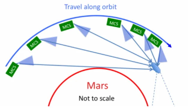
More importantly, from the perspective of MCS, the layer rises above the limb as the S/C approaches, reached a maximum altitude and then sets below the S/C. Figure 1 shows a schematic of the different views. This viewing geometry allows MCS to de-termine the altitude of the layer directly (to the 5 km vertical limb resolution). The actual altitude is the highest apparent height of the layer.

Figure 1. A diagram showing the location of the cloud within the MCS field of view over time. MCS (green) orbits from left to right as the location of the cloud starts low in the MCS field of view (blue), rises and then sets again.

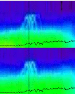
When the radiances are plotted in time (or lati-tude) order, the net result is that a detached, loca-lized haze layer appears to rise and then set (Figure 2). The MCS team calls the resulting structure an arch, although this is an illusion created by the view-ing geometry and the localized nature of the haze layer.

The arch in Figure 2 is a simple, well isolated, detached haze layer. MCS does not have the ability to determine the east-west extent of the haze unless

it is seen in an adjacent orbit ~27° away in longitude and 2 hours later (and even the it is necessary to as-sume it is the same haze and not a new one at a simi-lar latitude). The MCS resolution is ~3° in latitude due to the limb viewing geometry. For a haze layer at ~60 km, the arch structure will span ~20° in lati-tude. The actual width depends (weakly) on the height of the haze layer and the amount of low alti-tude opacity. In some cases (although not in Figure 2), it is possible to see the haze as a cold feature in absorption as it is setting (the right leg of the arch).

In many cases, there are complex structures with multiple narrow haze layers in a region. Figure 3 is an example of a case with at least 4 distinct overlap-ping arch structures. A separate haze layer generates each structure.

Figure 2. Brightness temperature based on the measured radiance in A1 (16.5 μm) on top and in A2 (15.9 μm) on the bottom. Green is ~180 K and dark purple/black is ~50 K with a rainbow between them. Each column is an individual 2 second MCS ra-diance measurement with all 21 detectors in the re-levant array. The views are shown with time in-creasing on the horizontal axis (covering ~30 mi-nutes). The vertical black line is the location of the equator. This is on the night side with MRO moving southward, so soundings to the right of the line are in the southern hemisphere. The jagged horizontal black lines are the location of the surface in the ar-ray at each sounding. This particular layer is at ~60 km and was observed at Ls = 117.2° (2006-10-07 12:54 UTC with an LMST of 03:00).

Layers with a height above 90 km would appear as a pair of arch “legs.” However so far none of the manual examinations of the radiances detected such features. There are even more complex structures seen in the data on some occasions. The current work does not attempt to address features that cannot be decomposed into individual arch structures.

Unfortunately the current MCS retrieval algo-rithm does not work in the region of the detached

haze layers. The current algorithm assumes a spher-ically symmetric atmosphere which is clearly not applicable in the presence of the localized haze layer. The current algorithm also does not retrieve CO2 ice, preventing it from correctly handling the spectroscopy of the haze in many cases.

Figure 3. Brightness temperature in A1 and A2. This is equivalent to Figure 2, for an orbit at Ls = 112.4°(2006-09-25 02:27 UTC). It also has an alti-tude of ~60 km and is centered on the equator.

Haze Climatology:

MCS has been observing fairly continuously for over 2 Mars Years so far. This spans from Ls = 111° in MY 28 (2006-09-24) through to the present (MY 30, Ls = 230°). Each day the instrument col-lects observations on 13 orbits, both daytime and nighttime, providing global coverage. Arch features are quite common in the dataset. In this work, we are using the observations to produce a climatology of the detached, localized haze layers.

In the appropriate seasons and regions, MCS de-tects haze layers as low as 10 km. There is usually sufficient opacity in the atmosphere (aerosol or ga-seous CO2 in the temperature sounding channels) to prevent the arch structure from being clearly re-solved below ~20 km.

At some seasons there are 50+ arch structures per day in the data. Figure 4 shows a manual analysis of 2 1/3 days (at the start of the MCS mission, Ls = 111°). 97 individual haze layers were identified during this time. The analysis catalogued the loca-tion, altitude, local time and the radiance profiles associated with each arch structure. An attempt was made to detect arches as faint as a few times the MCS noise level. This was possible by requiring the feature to have the time history of an arch in addition to the radiance maximum. The haze layers shown in Figure 3 are the vertical line of four arches at ~60 km (green) at -40 E on the equator.

number of apparent patterns. There are roughly equal numbers of arches in the daytime as at night. There appear to be four latitude bands/regions with layers in the night side. The northern mid-latitudes and polar regions, the equatorial region and southern

Adf Asdf As A A A A

Figure 4 (above). Location and approximate alti-tude of daytime arches over 2 1/3 days. The color represents the altitude. The dark purple is at ~10 km and each successive color is ~5 km higher.

aaa

Aaa Aaa

tropics. There is also a narrow band near 50 S and a few near the southern polar cap. Apart from the

band at 50 S, the same families appear in the day-time data. With one exception, the highest haze lay-ers are concentrated in equatorial regions and the layers on the day side are at higher altitudes than the larger population on the night side.

A preliminary and conservative automated search o

f

Figure 5 (below). Same as for Figure 4, but for the nighttime.

Haze Composition:

potential haze layers. Given the number, the team is currently working on automated arch detection and verification tools. This will not be as sensitive as the human search (due to the team’s lack of resources to develop a full expert system).

Haze Composition:

In addition to determining the location and alti-tude of a haze layer, the MCS radiances provide in-formation on the composition of the layer. The MCS channels are well designed to distinguish be-tween aerosols expected in the martian atmosphere (dust, water ice and CO2 ice). Many of the haze layers are only detected in some of the MCS chan-nels, and the rest of the layers have significantly different radiances at the various wavelengths. There are a number of issues that complicate the determination and a number of parameters that need to be considered. Since the particles can be emitting and scattering, an estimate of the layer temperature is necessary as well as the incident radiance. The actual properties (and thus the measured signal) also depend on the particle size. Finally, they depend on whether or not the layer is optically thick along the MCS limb path. (We assume they are all optically thin in the nadir path at the wavelengths of interest).

The MCS team has adopted a simplified ap-proach to automatically determining the composition of haze layers where possible. We have use a Mie calculation to determine the extinction efficiency (Qext), single scattering albedo (ω) and an integrated phase function (P) [Kleinböhl, et al., submitted] for a range of particle sizes. For ice (water or CO2), we use distributions with an reff from 0.125 μm to 8 μm; for dust we use a range from 0.133 μm to 6 μm.

We use the MCS observations to provide the ne-cessary input to the radiative transfer. We locate a nearby successful temperature retrieval (on the same orbit within 10° in latitude) to determine the emis-sive term. We locate a nearby on-planet view to estimate the upwelling radiance for scattering (with-in 2° and on the same orbit). In cases where either is not available, the automated determination of the composition is not possible.

When assuming the layer is optically thin, the ra-diance for each MCS channel showing the arch (plus the window channels) is fit using the following ex-pression:

Rl(η) = C Qext(η) *

[P(η) ω(η) Rs(η) + (1 - ω(η)) B(η,Tl)]

where η is the frequency or channel indicator, Rl is the limb radiance, Rs is the on-planet (top of atmos-phere) radiance, Tl is the temperature at the location of the layer and B Planck. C is a scaling constant related to the amount of haze in the layer. A given layer has a single scaling constant used for all chan-nels. For an optically thick layer, C = 1 and Qext is also set to 1.

The team then finds the best fit C parameter (the only free parameter), using a least squares criterion

on the difference of the log measured radiance – log calculated radiance. This is done for each particle size for each species and the RMS error of the best fit is calculated. For each particle size, the RMS error is also calculated for the optically thick case for each species. The species is that of the best fit (low-est RMS) case. While this also implicitly provides a particle size, the results are often flat (due to the limited MCS sensitivity to particle size). In doing this fitting, the team implicitly assumes the layer is either optically thin at all wavelengths or optically thick at all wavelengths.

The visible channel (A6) is not used in the com-position determination. It is very sensitive to scat-tered sunlight and often shows the strongest arch signature (on the daytime portion of the orbits). However, the scattered sunlight does not fit the sim-ple model used for estimating the arch radiance.

References:

Clancy et al. (2007), JGR 112, E04004, doi: 10.1029/2006JE002805.

Inada et al. (2007), Icarus 192, 378–395.

Kleinböhl et al. (2009), JGR 114, E10006, doi: 10.1029/2009JE003358.

Kleinböhl et al., J. Quant. Spectrosc. Radiat.

Transfer, submitted.

Määttänen et al. (2010), Icarus 209, 452–469, doi: 10.1016/j.icarus.2010.05.017.

McCleese et al. (2007), JGR, 112, E05S06 doi: 10.1029/2006JE002790.

McConnochie et al. (2009), Icarus 210, 545-565, doi: 10.1016/j.icarus.2010.07.021.

Montmessin et al. (2006) Icarus 183, 403–410. Montmessin et al. (2007), JGR 112, doi: 10.1029/2007JE002944.

Scholten et al. (2010), Planet. Space Sci. 58, 1207-1214, doi: 10.1016/j.pss.2010.04.015.

Zurek and Smrekar (2007), JGR, 112, E05S01, doi: 10.1029/2006JE002701.

Acknowledgement: This work was carried out at

the Jet Propulsion Laboratory, California Institute of Technology under a contract with the National Aeronautics and Space Administration.