Recipe for continuous monitoring of total ozone with a precision of around 1 DU applying mid-infrared solar absorption spectra

(1)

HAL Id: hal-00302908

https://hal.archives-ouvertes.fr/hal-00302908

Submitted on 26 Jun 2007

HAL is a multi-disciplinary open access

archive for the deposit and dissemination of sci-entific research documents, whether they are pub-lished or not. The documents may come from teaching and research institutions in France or abroad, or from public or private research centers.

L’archive ouverte pluridisciplinaire HAL, est destinée au dépôt et à la diffusion de documents scientifiques de niveau recherche, publiés ou non, émanant des établissements d’enseignement et de recherche français ou étrangers, des laboratoires publics ou privés.

Recipe for continuous monitoring of total ozone with a

precision of around 1 DU applying mid-infrared solar

absorption spectra

M. Schneider, F. Hase

To cite this version:

M. Schneider, F. Hase. Recipe for continuous monitoring of total ozone with a precision of around 1 DU applying mid-infrared solar absorption spectra. Atmospheric Chemistry and Physics Discussions, European Geosciences Union, 2007, 7 (3), pp.9093-9113. �hal-00302908�

(2)

ACPD

7, 9093–9113, 2007 Monitoring total ozone with a precision of around 1 DU

M. Schneider and F. Hase

Title Page Abstract Introduction Conclusions References Tables Figures ◭ ◮ ◭ ◮ Back Close

Full Screen / Esc

Printer-friendly Version Interactive Discussion

Atmos. Chem. Phys. Discuss., 7, 9093–9113, 2007 www.atmos-chem-phys-discuss.net/7/9093/2007/ © Author(s) 2007. This work is licensed

under a Creative Commons License.

Atmospheric Chemistry and Physics Discussions

Recipe for continuous monitoring of total

ozone with a precision of around 1 DU

applying mid-infrared solar absorption

spectra

M. Schneider and F. Hase

IMK-ASF, Forschungszentrum Karlsruhe, Karlsruhe, Germany

Received: 20 April 2007 – Accepted: 18 June 2007 – Published: 26 June 2007 Correspondence to: M. Schneider (matthias.schneider@imk.fzk.de)

(3)

ACPD

Full Screen / Esc

Printer-friendly Version Interactive Discussion Abstract

Mid-infrared solar absorption spectra recorded by a state-of-the-art ground-based FTIR system have the potential to provide precise total O3 amounts. The currently

best-performing retrieval approaches use a combination of small and broad spectral O₃ windows between 780 and 1015 cm−1

. We show that for these approaches

uncertain-5

ties in the temperature profile are by far the major error sources. We demonstrate that a joint optimal estimation of temperature and O₃ profiles widely eliminates this error. The improvements are documented by an extensive theoretical error estimation. Our results suggest that mid-infrared FTIR measurements can provide total O3 amounts

with a precision of around 1 DU, placing this method among the most precise

ground-10

based O3 monitoring techniques. We recapitulate the requirements on instrumental

hardware and retrieval necessary to achieve this high precision.

1 Introduction

The demand for very high precision measurements of atmospheric constituents is re-cently increasing. Many aspects of stratospheric ozone destruction (and recovery)

15

or the evolution of atmospheric greenhouse gases are well understood. However, a closer look reveals important uncertainties. Concerning ozone recovery, it is not clear how climate change will affect upper tropospheric and stratospheric ozone amounts. Consequently, it cannot be foreseen how, when, and to what extent ozone recovery will take place (Weatherhead and Andersen,2006). Very high precision measurements are

20

important for further scientific progress. They are indispensable to document potential differences between the real and a modeled atmosphere in due time.

Ground-based measurements yielding highly-resolved infrared solar absorption spectra allow ongoing detection of the composition of the atmosphere in a cost-effective manner. They are essential for validating satellite measurements and, thus, they are

25

a vital component of the global atmospheric monitoring system. Ongoing improve-9094

(4)

ACPD

Full Screen / Esc

ments in instrumental hardware, spectroscopic parameterisation, and retrieval strate-gies steadily increase the FTIR data quality. In this work we estimate the potential of high quality middle infrared spectra for a precise monitoring of total O3 amounts. The

estimations base on the spectra quality routinely achieved with a Bruker IFS 125HR at the Iza ˜na Observatory, Canary Island of Tenerife, Spain. In the following Sections we

5

describe the current state-of-the-art O3 profile retrieval (De Mazi `ere et al.,2004) and

estimate its errors. The error estimation motivates to set up a new retrieval strategy, which includes the optimal estimation of temperature profiles. We predict that the new approach should allow for the retrieval of FTIR O3column amounts with a precision of

around 1 DU. In Sect. 4 we summarize in detail the requirements on the

instrumen-10

tal hardware and the kind of retrieval strategy necessary in order to achieve this high precision.

2 Optimal estimation of O₃profiles

2.1 Retrieval strategy

We apply an optimal estimation (OE) method (Rodgers, 2000) to invert the profiles

15

from the measured FTIR spectra by minimising the cost function: σ−2_{(y − Kx)}T_{(y − Kx) + (x − x}

a)TSa−1(x − xa) (1)

The first term considers the information present in the spectra assuming a diagonal noise covariance (K, y, and σ represent Jacobian, the spectrum, and the measurement noise, respectively). The second term accounts for the a-priori knowledge: S_ais the

a-20

priori covariance matrix, and x and xa, represent the state vector and the a-priori state.

We apply the inversion code PROFFIT (Hase et al.,2004) which uses the Karlsruhe Optimised and Precise Radiative Transfer Algorithm (KOPRA, H ¨opfner et al., 1998; Kuntz et al.,1998;Stiller et al.,1998) as the forward model.

(5)

ACPD

Full Screen / Esc

We use spectral microwindows with 48O3 and asymmetric and symmetric 50

O3 and 49

O₃ absorption signatures in the mid-infrared (between 780–1015 cm−1_{; see Fig.} _1).

In the 782.75 and 789.0 cm−1

windows only the main isotopologue (48O3) has

absorp-tion signatures. There are also minor interferences from CO2, H2O, and solar lines.

These two microwindows are the same that were used inSchneider et al.(2005). The

5

strongest line in the 993.5 cm−1

window is a symmetric50O3signature (at 993.8 cm−1).

Other signatures are from 48O3, asymmetric 50

O3, symmetric and asymmetric 49

O3,

H₂O, CO₂, and solar lines. Broadband microwindows are very useful to improve the sensitivity of the observing system for the lower troposphere (Barret et al.,2002). We apply three broadband microwindows between 1000.0 and 1013.6 cm−1_{. There all}

10

48

O₃,50O₃, and49O₃isotopologues have absorption signatures. The main interfering species are H2O and CO2.

We make an OE of48O3, asymmetric, and symmetric 50

O3 and of the isotopologue

ratio profiles of 48O₃/50O₃. The latter is an option recently introduced in PROFFIT (Schneider et al., 2006), which provides for an improved constraint of the resulting

15

profiles. As a-priori of O3 (mean profile and covariances) we use a climatology of

Iza ña’s ECC-sondes from 1996 to 2006, i.e. in a strict sense the retrieval is optimised for the Iza ña site. However, in this and the following Section we show that the choice of the a-priori is a minor error source and consequently our conclusions are not limited to Iza ña. As a-priori for the typical ozone isotopologue ratio profiles and their covariances

20

we use data reported byJohnson et al.(2000). The spectral signatures of the minor isotopologues of49O3are only considered by scaling a climatological profile. The H2O

interferences are considered by scaling an actual H₂O profile as retrieved in a previous step from specific H₂O microwindows of the same measurement. This H₂O retrieval is described inSchneider et al. (2006). The minor signatures of CO2 and C2H4 are

25

considered by scaling corresponding climatological profiles.

The applied temperature data are a combination of the data from the local ptu-sondes (up to 30 km) and data supplied by the automailer system of the Goddard

(6)

ACPD

Full Screen / Esc

Space Flight Center. The spectroscopic line parameters of H₂O and of O₃ are taken from the HITRAN 2004 database (Rothman et al., 2005). For all other species we apply HITRAN 2000 parameters (Rothman et al.,2003). To minimize errors due to un-certainties of the instrumental line shape we measure and eventually correct line shape distortions regularly every two months. These measurements consist in independent

5

detections of cell absorption signatures as described inHase et al. (1999). The σ of Eq. (1) is taken from the residuals of the fit itself, performing an automatic adjustment of the constraints according to the noise level found in each measurement.

2.2 Error estimation

Our error analysis bases on the analytic method suggested byRodgers(2000), where

10

the difference between the retrieved and the real state ( ˆx − x) – the error – is linearised about a mean profile xa, the estimated model parameters ˆp, and the measured

spec-trum ˆy: ˆ x − x = ( ˆA − I)(x − xa) 15 + ˆG ˆK_p(p − ˆp) + ˆG(y − ˆy) (2)

Here I is the identity matrix, ˆA the averaging kernel matrix, ˆG the gain matrix, and ˆ

K_p a sensitivity matrix to model parameters. Equation (2) identifies the three principle error sources. These are: (a) errors due to the inherent finite vertical resolution of

20

the observing system (smoothing error), (b) errors due to uncertainties in the input parameters applied in the inversion procedure, and (c) errors due to measurement noise.

Generally one assumes linearity of the forward model within the range of the vari-ability of the atmospheric state. Then the errors are calculated according to Eq. (2)

25

applying single mean matrices for ˆA, ˆG, and ˆK_p. However, for the saturated (or nearly 9097

(7)

ACPD

Full Screen / Esc

saturated) spectral O₃ lines as shown in Fig. 1 the Jacobians depend on the actual atmospheric state. Therefore, we use an ensemble of 500 real states which obeys the a-priori statistics and calculate for each individual members of this ensemble the matrices ˆA, ˆG, and ˆK_p: we make for each of the 500 real states an individual error estimation according to Eq. (2).

5

Errors generally have a systematic and a random component. These components can easily be separated by correlating an input column amount to the actually retrieved column amount. The systematic error component is then given by the linear regres-sion line of the least square fit. By input amount we refer to the amount that would be retrieved in the absence of the considered error. There are two types of systematic

10

errors: (a) the “sensitivity error”, which is given by the differences of the slope of the regression line from unity. It reveals how the observing system systematically over-/underestimates the deviations from the a-priori value. (b) the “bias error”, which gen-erates an offset in the regression line at the a-priori value (climatological mean value). The “bias error” is due to systematic error sources or incorrect a-priori assumptions.

15

The scattering around the regression line gives the random error. For the estimation of the random error component we recall Eq. (5) ofSchneider et al.(2006):

σ_ǫ_reg _{= σ}_x_ˆ q

1 − ρ2 ₍₃₎

It links the correlation coefficient ρ to the scattering around the regression line, i.e. to the random error component σ_ǫ_reg. For more details about this method of error

calcu-20

lations please consultSchneider et al.(2006).

2.2.1 Smoothing error

For each member of our ensemble of real states x we calculate a retrieved state ˆ

x_{= ˆA(x−x}_a_)+x_a. Panel (a) of Fig. 2 shows the correlation between the total column amount calculated from the real state (input column amount) and the total column

25

amount calculated from ˆx (retrieved total column amount). The smoothing error has 9098

(8)

ACPD

Full Screen / Esc

no systematic “bias error” component (no offset between real and retrieved state at a-priori value). This is trivial, since we use as a-a-priori the same statistics that was applied for the simulation of the ensemble profiles. However, it is not trivial that there is nearly no systematic “sensitivity error” (slope of regression line of 0.998). This nearly perfect sensitivity demonstrates that the choice of the a-priori has a negligible impact on the

5

retrieved O3 amounts. A correlation coefficient ρ of 0.99989 and a typical variability

of the retrieved total column amount σxˆ of 24 DU leads, according to Equation 3 to

an random error σ_ǫ_reg of 0.36 DU. The estimated systematic and random smoothing errors are listed together with the other errors in Table2.

2.2.2 Input parameter errors

10

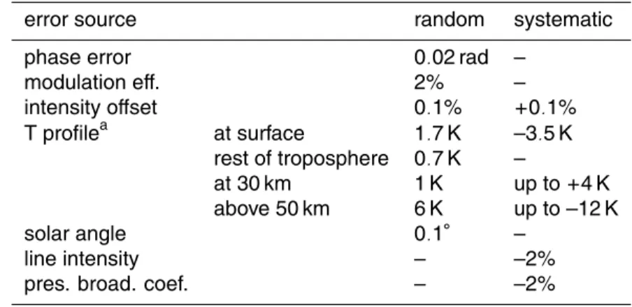
In this Subsection errors due to uncertainties in solar angle, instrumental line shape (ILS: modulation efficiency and phase error,Hase et al.,1999), baseline of the spec-trum (intensity offset), temperature profile, and spectroscopic parameters (line intensity and pressure broadening coefficient) are estimated. The assumed parameter uncer-tainties (p− ˆp) are listed in Table1.

15

We estimate the ILS stability from regularly performed low pressure N2O cell

mea-surements (Hase et al.,1999), to 0.02 rad for the phase error and 2% for the modulation efficiency. An intensity offset may be caused by detector non-linearities. Here we use a photo-voltaic MCT detector instead of the usually applied photo-conductive detectors. It has the advantage of reduced non-linearities and thus an improved zero baseline

de-20

termination (less spectral intensity offset). We estimate the spectral intensity offset in our spectra by analysing very intense O3signatures between 1024.25 and 1025 cm−1.

Those signatures are saturated even for O3slant columns as low as 250 DU. We found

a mean offset of 0.1% and a standard deviation of 0.1% in the core of the saturated lines. Two sources are considered as random uncertainty in the temperature profile:

25

first, the measurement uncertainty of the sonde, which is assumed to be 0.5 K through-out the whole troposphere and to have no interlevel correlations. Second, the temporal differences between the FTIR and the sonde’s temperature measurements, which are

(9)

ACPD

Full Screen / Esc

estimated to be 1.5 K at the surface and 0.5 K in the rest of the troposphere, with a correlation length 5 km. Furthermore, we assume systematic errors in the temperature profile (for more details please see Sect.3).

We estimate the impact of the parameter uncertainties as listed in Table1by correlat-ing the input column amounts to the retrieved column amounts. Here the input column

5

amount is the amount retrieved in the absence of parameter errors, i.e. the smoothed real amount ( ˆx_{= ˆA(x−x}_a_)+x_a). The retrieved amounts are the amounts retrieved in the presence a parameter error ( ˆx_{+ ˆ}G ˆK_p(p− ˆp)). The correlations are shown in panels (b) to (h) of Fig.2. The systematic and random errors are estimated as for the smoothing error: from the slope and bias of the regression line and the correlation coefficient (see

10

Eq.3). The assumed uncertainties of Table1lead to large random and systematic er-rors due to uncertainties in the temperature profile (random: 3.5 DU; “sensitivity error”: –3.3%; bias: −7.0 DU). We also made these simulation assuming no systematic error in the temperature profile, i.e. assuming no error for the temperature dependance of the pressure broadening coefficient. In this case the random error remains unchanged

15

at 3.5 DU, but the systematic components reduce significantly: to −1.6% for the “sen-sitivity error” and to −0.2 DU for the bias. Although reduced, there is still a systematic sensitivity error even in the absence of a systematic temperature error source. The reason might be the large impact of temperature on the simulated spectrum: a wrong temperature assumption produces significant discrepancies between measured and

20

simulated spectra, which reduce the sensitivity of the observing system.

Error sources of minor importance are the intensity offset, solar elevation angle, and modulation efficiency (0.4, 0.3 and 0.3 DU, respectively). All other random errors are negligible, i.e. are situated below 0.2 DU. Significant systematic errors are produced by errors in the line intensity parameter (error of 2% column amount error for 2%

pa-25

rameter error) and due to an intensity offset (error of −0.2% for assumed systematic offset of 0.1%). A systematic error in the pressure broadening coefficient causes only very small systematic errors in the column amounts. All errors are collected in Table2.

(10)

ACPD

Full Screen / Esc

2.2.3 Measurement noise error

This error is due to statistical fluctuation in the measured signal, caused by e.g. photon noise or thermal noise in the detector or noise produced by the signal amplification. It causes white noise in the residuals. With the Bruker IFS 125HR and the applied photo-voltaic MCT detector we reach a signal to noise ratio of better than 600 around

5

1000 cm−1_{. We found this value by analysing measured spectra in regions with no}

absorption issues. Its impact on total column amounts is negligible. Our simulations lead to errors around 0.1 DU (see Table2).

3 Simultaneous optimal estimation of O₃and temperature profiles

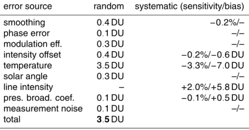
Table2 reveals that uncertainties in the assumed temperature profile are mainly

re-10

sponsible for the overall errors in the retrieved columns amounts. Both the shape and the intensity of an absorption line depend on the temperature. Thus, errors in the tem-perature profile lead to erroneous simulations of the line shapes and intensities and consequently to errors in the retrieved trace gas profiles.

The applied inversion code PROFFIT allows a joint optimal estimation of

tempera-15

ture profile together with VMR profiles. From the viewpoint of the forward model, the retrieval of temperature brings in several complications: the absorption cross sections cannot be precomputed before the iterative retrieval process is performed, instead re-calculation in each iteration step is required. Derivatives of temperature have to be provided at each model level. The construction of the temperature derivatives within

20

the forward model KOPRA used here, is described inStiller et al. (2000). Finally, as hydrostatic equilibrium is assumed, it has to be taken into account that a change of the temperature profile implicates a modified pressure stratification. Therefore, in each it-eration step an atmosphere in hydrostatic balance is reconstructed and the pressure at each altitude fixed model level is changed according to the current temperature profile.

25

From the viewpoint of the retrieval, the joint fit of temperature requires extensions to the 9101

(11)

ACPD

Full Screen / Esc

state vectors, the Jacobian and the a-priori covariances. An a-priori temperature profile and associated a-priori covariance have to be provided by the user as additional input. The a-priori temperature profiles used here are a combination of the daily ptu-sonde and the Goddard NCEP temperatures as described in Sect.2. The a-priori tempera-ture covariance is constructed in accordance with the assumed random error budget of

5

the temperature profile (see Table1). The reasons for the random temperature errors are described in Sect.2. We also found systematic differences between our optimally estimated temperature profiles and the ptu-sonde/NCEP temperature profiles, which we interpreted as systematic temperature errors. There are several reasons for these differences: (a) the ptu-sonde measures in the free troposphere while the FTIR is a

10

ground-based instrument. At the sonde’s location the temperature is generally below the temperature at the FTIR site. (b) At higher altitudes the sonde may give to large temperatures due to radiative heating (c) The Goddard NCEP temperatures may have systematic errors. (d) The parameterisation of the temperature dependence of the lines may be erroneous. Such a systematic error in the spectroscopic data produces

15

systematic differences between actual and retrieved temperature profile.

We analyse how a joint optimal estimation of the temperature profiles reduces the impact of temperature uncertainties on the retrieved O3column amounts. We calculate

for all 500 members of the ensemble the matrices ˆA, ˆG, and ˆK_p for the new retrieval setup and perform the same error simulation as in Sect.2. We found that an OE

es-20

timation of the temperature applying the O₃ windows of Fig. 1 already reduces the temperature error. However, an additional application of CO2windows should yield to

further improvements. Spectral signatures of CO2 are often used in remote sensing

to determine temperature profiles. Atmospheric CO2 is very stable. It has little

tem-poral variability and its mixing ratios are nearly constant over large altitude regions.

25

Changes in the CO2 absorption pattern can thus be mainly attributed to changes in

the temperature profile. Furthermore, CO2is an infrared active gas and its

concentra-tions are relatively high which assures distinct absorption signatures. We apply four spectral windows between 960 and 970 cm−1 _{containing isolated CO}

2lines of different

(12)

ACPD

Full Screen / Esc

intensities (see Fig.3) together with the windows as described in Sect. 2and shown in Fig. 1. The only significantly interfering absorptions in the CO2 windows are due

to O3 and can be seen as the tiny dips in the 969 cm−1 window. To adjust the

mea-sured and simulated CO2 signatures we only allow a scaling of a climatological CO2

profile: inconsistencies between the four CO₂ line intensities and in their line shapes

5

are considered by adapting the temperature profile.

For this retrieval setup the errors due to temperature uncertainties are widely elimi-nated. The random error is reduced from 3.5 DU to 0.1 DU. The systematic sensitiv-ity error is reduced from −3.3% to −0.2% and the systematic bias from −7.0 DU to −0.4 DU. The smoothing error, the intensity offset, and errors due to uncertainties in

10

the ILS and the solar elevation angle remain as leading error sources. For the assump-tions listed in Table 1 we estimate a total random error of around 1.2 DU. This is a significant improvement over the current state-of-the-art retrieval method for which we estimate a total random error of 3.5 DU. All errors are listed in Table3.

4 Summary and conclusions

15

Applying a state-of-the-art instrumentation and retrieval strategy provides for an esti-mated precision of total O₃ of around 1DU, which converts the FTIR technique to one of the most precise techniques for a continuous monitoring of total O3. From Table 3

we conclude that important remaining error sources are intensity offsets, small uncer-tainties of the ILS or of the solar elevation angle, and the smoothing error. It is,

further-20

more, important to state that we estimate a near ideal column sensitivity. Therefore, the applied a-priori has negligible influence on the retrieved O3 amounts. All

informa-tion about the actual O₃ content is taken from the measurement and consequent our error estimation is of general validity and not limited to the Iza ˜na site. The recipe is summarized as follows and contains retrieval and instrumental aspects:

25

1. To eliminate the temperature error and to keep the smoothing error small it is 9103

(13)

ACPD

Full Screen / Esc

required to apply a retrieval strategy as described in the previous Sections, i.e. it is mandatory to apply broad spectral windows and to perform a joint OE of48O3, 48

O3/ 50

O3, and temperature profiles. Therefore one should apply additionally the

spectral CO₂windows as shown in Fig.3. The joint OE of the temperature profile provides for the decisive improvement of the precision. Currently PROFFIT (Hase

5

et al., 2004) is the only retrieval code for the analysis of ground-based spectra that allows to perform an OE of temperature and isotopologue profiles.

2. One should apply a photo-voltaic instead of a photo-conductive detector. Photo-voltaic detectors have a quite linear characteristics whereas photo-conductive de-tectors show a certain level of non-linearity, which may introduce baseline

arte-10

facts into the spectra.

3. The intensity fluctuations during scanning should be documented. For example, clouds passing through the line of sight during scanning may cause intensity off-sets in the spectra. A correction of these baseline artefacts is only possible if in addition to the AC interferogram signal the DC interferogram signal is recorded.

15

At Iza ˜na such a correction was not necessary due to the nearly continuous per-fect clear sky conditions, however at sites with less favorable sky conditions it is indispensable.

4. One should use an instrument with a stable ILS like the Bruker IFS 120/125HR. Currently the Bruker IFS 120/125 HR spectrometers are among the

best-20

performing FTIR spectrometers commercially available. It is difficult to achieve the required stability with portable instruments like a Bruker IFS 120M.

5. The pointing of the solar tracker and the effective measurement time should be known with high accuracy. For a solar elevation angle of 40◦

an uncertainty of 0.1◦

in the pointing or of 30 seconds in the effective measurement time causes

25

an error of 0.3 DU. For an elevation angle of 20◦ _{or 10}◦ _{this error increases to}

0.7 DU and 1.2 DU, respectively. At Iza ˜na we apply an high quality home-built 9104

(14)

ACPD

Full Screen / Esc

solar tracker. Its mirror positions are determined from astronomical calculations and additionally controlled by the signals of a quadrant detector (Huster,1998). Finally, it should be commented that a further reduction of the noise level would yield no further improvement: as shown in Table 3 the measurement noise is a negligible error source.

5

Acknowledgements. We would like to thank the European Commission for funding via the

project GEOMON (contract GEOMON-036677). Furthermore, we are grateful to the Goddard Space Flight Center for providing the temperature and pressure profiles of the National Centers for Environmental Prediction via the automailer system.

References

10

Barret, B., De Mazi `ere, M., and Demoulin, P.: Retrieval and characterization of ozone profiles from solar infrared spectra at the Jungfraujoch, J. Geophys. Res, 107, 4788–4803, 2002.

9096

De Mazi `ere, M., Barret, B., Vigouroux., C., Blumenstock, T., Hase, F., Kramer, I., Camy-Peyret, C., Chelin, P., Gardiner, T., Coleman, M., Woods, P., Ellingsen, K., Gauss, M., Isaksen, I.,

15

Mahieu, E., Demoulin, P., Duchatelet, P., Mellqvist, J., Strandberg, A., Velazco, V., Schulz, A., Notholt, J., Sussmann, R., Stremme, W., and Rockmann, A.: Ground-based FTIR mea-surements of O₃and climate related gases in the free troposphere and lower stratosphere, presented at the Quadrenial Ozone Symposium in Kos, Greece, from June 1st to 8th 2004.

9095

20

Hase, F., Blumenstock, T., and Paton-Walsh, C.: Analysis of the instrumental line shape of high-resolution Fourier transform IR spectrometers with gas cell measurements and new retrieval software, Appl. Opt., 38, 3417–3422, 1999. 9097,9099

Hase, F., Hannigan, J. W., Coffey, M. T., Goldman, A., H ¨opfner, M., Jones, N. B., Rinsland, C. P., and Wood, S. W.: Intercomparison of retrieval codes used for the analysis of high-resolution,

25

ground-based FTIR measurements, J. Quant. Spectrosc. Radiat. Transfer, 87, 25–52, 2004.

9095,9104

H ¨opfner, M., Stiller, G. P., Kuntz, M., Clarmann, T. v., Echle, G., Funke, B., Glatthor, N., Hase, F., Kemnitzer, H., and Zorn, S.: The Karlsruhe optimized and precise radiative transfer

(15)

ACPD

Full Screen / Esc

gorithm, Part II: Interface to retrieval applications, SPIE Proceedings 1998, 3501, 186–195, 1998. 9095

Huster, S. M.: Bau eines automatischen Sonnenverfolgers f ür bodengebundene IR-Absorptionmessungen, Diplomarbeit im Fach Physik, Institut f ür Meteorologie und Kli-maforschung, Universit ät Karlsruhe und Forschungszentrum Karlsruhe, 1998. 9105

5

Johnson, D. G., Jucks, K. W., Traub, W. A., and Chance K. V.: Isotopic composition of strato-spheric ozone, J. Geophys. Res., 105, 9025–9031, 2000. 9096

Kuntz, M., H ¨opfner, M., Stiller, G. P., Clarmann, T. v., Echle, G., Funke, B., Glatthor, N., Hase, F., Kemnitzer, H., and Zorn, S.: The Karlsruhe optimized and precise radiative transfer al-gorithm, Part III: ADDLIN and TRANSF algorithms for modeling spectral transmittance and

10

radiance, SPIE Proceedings 1998, 3501, 247–256, 1998.9095

Rodgers, C. D.: Inverse Methods for Atmospheric Sounding: Theory and Praxis, World Scien-tific Publishing Co., Singapore, 2000. 9095,9097

Rothman, L. S., Barbe, A., Benner, D. C., Brown, L. R., Camy-Peyret, C., Carleer, M. R., Chance, K. V., Clerbaux, C., Dana, V., Devi, V. M., Fayt, A., Fischer, J., Flaud, J.-M.,

15

Gamache, R. R., Goldman, A., Jacquemart, D., Jucks, K. W., Lafferty, W. J., Mandin, J.-Y., Massie, S. T., Newnham, D. A., Perrin, A., Rinsland, C. P., Schroeder, J., Smith, K. M., Smith, M. A. H., Tang, K., Toth, R. A., Vander Auwera, J., Varanasi, P., and Yoshino, K.: The HITRAN Molecular Spectroscopic Database: Edition of 2000 Including Updates through 2001, J. Quant. Spectrosc. Radiat. Transfer, 82, 5–44, 2003.9097

20

Rothman, L. S., Jacquemart, D., Barbe, A., Benner, D. C., Birk, M., Brown, L. R., Carleer, M. R., Chackerian Jr., C., Chance, K. V., Coudert, L. H., Dana, V., Devi, J., Flaud, J.-M., Gamache, R. R., Goldman, A., Hartmann, J.-M., Jucks, K. W., Maki, A. G., Mandin, J.-Y., Massie, S. T., Orphal, J., Perrin, A., Rinsland, C. P., Smith, M. A. H., Tennyson, J., Tolchenov, R. N., Toth, R. A., Vander Auwera, J., Varanasi, P., and Wagner, G.: The HITRAN 2004 molecular

25

spectroscopic database, J. Quant. Spectrosc. Radiat. Transfer, 96, 139–204, 2005. 9097

Schneider M., Blumenstock, T., Hase, F., H ¨opfner, M., Cuevas, E., Redondas, A., and San-cho, J. M.: Ozone profiles and total column amounts derived at Iza ˜na, Tenerife Island, from FTIR solar absorption spectra, and its validation by an intercomparison to ECC-sonde and Brewer spectrometer measurements, J. Quant. Spectrosc. Radiat. Transfer, 91, 245–274,

30

2005. 9096

Schneider, M., Hase, F., Blumenstock, T.: Ground-based remote sensing of HDO/H2O ratio profiles: introduction and validation of an innovative retrieval approach, Atmos. Chem. Phys.,

(16)

ACPD

Full Screen / Esc

6, 4705–4722, 2006,

http://www.atmos-chem-phys.net/6/4705/2006/. 9096,9098

Stiller, G. P., H ¨opfner, M., Kuntz, M., Clarmann, T. v., Echle, G., Fischer, H., Funke, B., Glatthor, N., Hase, F., Kemnitzer, H., and Zorn, S.: The Karlsruhe optimized and precise radiative transfer algorithm, Part I: Requirements, justification and model error estimation, SPIE

Pro-5

ceedings 1998, 3501, 257–268, 1998. 9095

Stiller, G. P. (Editor) with contributions from T. v. Clarmann, A. Dudhia, G. Echle, B. Funke, N. Glatthor, F. Hase, M. Hpfner, S. Kellmann, H. Kemnitzer, M. Kuntz, A. Linden, M. Linder, G. P. Stiller, S. Zorn: The Karlsruhe Optimized and Precise Radiative transfer Algorithm (KO-PRA), Forschungszentrum Karlsruhe, Wissenschaftliche Berichte, Bericht Nr. 6487, 2000.

10

9101

Weatherhead, E. C and Andersen, S. B.: The search for signs of recovery of the ozone layer, Nature, 441, 39–45, 2006. 9094

(17)

ACPD

Full Screen / Esc

Printer-friendly Version Interactive Discussion Table 1. Assumed uncertainties.

error source random systematic phase error 0.02 rad –

modulation eff. 2% – intensity offset 0.1% +0.1% T profilea at surface 1.7 K –3.5 K rest of troposphere 0.7 K – at 30 km 1 K up to +4 K above 50 km 6 K up to –12 K solar angle 0.1◦ _– line intensity – –2% pres. broad. coef. – –2%

a

detailed description see text

(18)

ACPD

Full Screen / Esc

Printer-friendly Version Interactive Discussion Table 2. Estimated random (in DU) and systematic errors (sensitivity in % and bias in DU) of

the total column amounts.

error source random systematic (sensitivity/bias) smoothing 0.4 DU _−0.2%/– phase error 0.1 DU –/– modulation eff. 0.3 DU –/– intensity offset 0.4 DU _{−0.2%/−0.6 DU} temperature 3.5 DU −3.3%/−7.0 DU solar angle 0.3 DU –/– line intensity – +2.0%/+5.8 DU pres. broad. coef. 0.1 DU −0.1%/+0.5 DU measurement noise 0.1 DU –/– total 3.5 DU

(19)

ACPD

Full Screen / Esc

Printer-friendly Version Interactive Discussion Table 3. Estimated random (in DU) and systematic errors (in %) of O₃total column amounts

for simultaneous optimal estimation of O₃and temperature profiles.

error source random systematic (sensitivity/bias) smoothing 0.5 DU –/– phase error 0.3 DU –/– modulation eff. 0.7 DU +0.1%/– intensity offset 0.6 DU +0.3%/−0.9 DU temperature 0.1 DU −0.2%/−0.4 DU solar angle 0.3 DU –/– line intensity – +2.0%/+5.7 DU pres. broad. coef. 0.1 DU −0.1%/+0.3 DU measurement noise 0.1 DU –/– total 1.2 DU

(20)

ACPD

Full Screen / Esc

Printer-friendly Version Interactive Discussion Fig. 1. Spectral windows applied. Plotted is the situation for a real measurement taken on

22 January 2005 (solar elevation angle 32.2◦_{; black line: measured spectrum; dotted red line:}

simulated spectrum; blue line: difference between simulation and measurement.

(21)

ACPD

Full Screen / Esc

Printer-friendly Version Interactive Discussion Fig. 2. Correlation plots for the estimation of the random and systematic errors. Circles

repre-sent the 500 individual members of the applied ensemble; red lines the linear regression line. Black dashed line indicates the diagonal, i.e. the situation for no systematic error component.

(22)

ACPD

Full Screen / Esc

Printer-friendly Version Interactive Discussion Fig. 3. Applied CO₂ windows. The spectra correspond to the same measurement as the

spectra shown in Fig.1. Scale and meaning of lines and colours is the same as in Fig.1