Habits and rational behavior in residential electricity
demand
M. Filippini 1 B. Hirl 2 G. Masiero 3
Published in:
Resource and Energy Economics (2018), 52: 137-152. < https://doi.org/doi:10.1016/j.reseneeco.2018.01.002 >
Abstract
Households make an investment analysis when buying new electrical appli-ances. Therefore, expectations about future electricity consumption may have an impact on current consumption and investment decisions. Dynamic partial adjustment models of residential electricity demand neglect rational consumer behavior. In this paper we propose a model for residential electricity demand that allows for forward-looking behavior. We estimate lead consumption models using two stages least squares fixed effects on a panel of 48 US states between 1995 and 2011. We find that expectations about future consumption have an impact on current consumption decisions. This novel approach may improve our understanding of the dynamics of residential electricity demand and the evalua-tion of the effects of energy policies.
JEL classification: D12, D84, D99, Q41, Q47, Q50
Keywords: Residential electricity, Partial adjustment models, Dynamic panel data models, Rational habits
1Institute of Economics (IdEP), Università della Svizzera italiana (USI); Department of
Manage-ment, Technology and Economics, ETH Zurich, Switzerland.
2Institute of Economics (IdEP), Università della Svizzera italiana (USI). Corresponding author.
E-mail address: [email protected]. We thank the editor and two anonymous reviewers for their many insightful comments and suggestions that allowed us to improve the paper.
3
Department of Management, Information and Production Engineering (DIGIP), University of Bergamo, Italy; Institute of Economics (IdEP), Università della Svizzera italiana (USI), Switzerland.
1
Introduction
In the US, residential electricity consumption accounts for about a third of total elec-tricity consumption. Understanding the dynamics of household energy consumption is of great importance in formulating policies to improve the efficient use of energy services. Households use energy services (e.g. lighting, TV entertainment, cooling of food, hot water) by combining electrical appliances and electricity. Therefore, house-holds face simultaneous consumption and investment decisions: how much energy to consume and what stock of electrical appliances to hold. Their reaction to a chang-ing environment, such as an increase in the price of electricity, may then lead to an adjustment in the stock of electrical appliances or a change in their use. For instance, they may decide to switch to a more energy efficient lighting system, or they may adjust their consumption habits by switching off the light more often when leaving a room. In this paper, we propose a model for residential electricity demand that allows for forward-looking behavior, and estimate this model using two stage least squares fixed effects on a panel of US states.
When making current consumption and investment decisions, households look at the constant maximization of utility over time (Becker and Murphy, 1988) and take expectations about future electricity consumption into account. A household’s energy consumption reflects the efficiency of its capital stock. Investments in more efficient appliances will allow to produce (today and in the future) the same energy services with a lower amount of energy. Therefore, a household that optimizes utility over time will adjust today’s consumption to lower levels.
In addition, because of habits or the constraint related to changing the stock of electrical appliances, current consumption decisions are affected by past consumption. Households may not be able to change their electricity consumption or to adjust their stock of electrical appliances fast enough to instantaneously react to changes in the price of electricity. This slow adjustment process may also reflect bounded rationality or status quo bias, i.e. consumers make use of available information but their decision-making is bounded by habits, inertia, or a general aversion to change (Samuelson and Zeckhauser, 1988; Kahneman et al., 1991).
The recent literature on residential electricity demand neglects forward-looking household behavior (e.g., Alberini and Filippini, 2011; Blázquez et al., 2013; Cebula, 2012). Generally, residential electricity demand is estimated using static models, where no interdependence of consumption decisions over time is assumed, or using dynamic partial adjustment models that account only for the impact of past
tion. Two recent studies that consider forward-looking behavior in energy consump-tion are Scott (2012, 2015), but the analyses focus on gasoline rather than electricity and the econometric approaches rely on lead price models, where current consumption is affected by future prices, rather than lead consumption models, where current and future consumption are interdependent.
This analysis builds on the literature on rational habits (e.g., Becker et al., 1994) to extend and generalize the existing dynamic partial adjustment approach to electric-ity demand by considering expectations about future consumption. To this aim, we estimate and compare three main models: a static model, a myopic model and a lead consumption model. Our novel approach based on the lead consumption model seems to provide more precise estimates of the dynamics of residential electricity consump-tion. Not only do we capture the effects of behavioural habits and constraints of the current stock of appliances but also of the behavioural adjustment to the future. We show that expectations about changes in future consumption significantly influence current consumption, which suggests evidence of forward-looking household behavior. Clearly, forward-looking behavior does not imply that households have perfect fore-sight or are completely rational. Expectations about the future may be flawed and agents may be bounded in taking into account information about the future. Rather than rely on a perfect optimization process, it seems reasonable to assume that agents use simple decision rules that include some expectations about the future.
Our findings suggest that households adjust today’s consumption in response to changes in the future, such as the implementation of new energy and environmental policies. This has potentially important impacts for policy analysis and evaluation. For instance, if the policy maker announces the introduction of a future environmental tax, households may modify their electricity consumption before the tax is introduced. Note that policy evaluation methods such as difference-in-difference may underesti-mate the full impact of a policy since the anticipation effect on electricity consumption is generally neglected. The policy maker should then consider this effect when design-ing and implementdesign-ing energy policy measures. Even when the implementation period of a policy is relatively long due to political and administrative constraints, the policy may have immediate effects.
The remainder of the essay is organized as follows. Section 2 gives an overview of the existing literature on residential electricity consumption. In section 3 we derive a forward-looking model of residential electricity consumption. Section 4 presents the empirical approach and describes the data, and section 5 discusses the econometric estimation. The results are summarized and discussed in section 6, while section 7
concludes the essay.
2
Residential electricity demand in the literature
Residential electricity demand has been studied extensively in the economic literature. Since the early works of Houthakker (1951), Fisher and Kaysen (1962) and Mount et al. (1973), the focus of most studies has been the relationship between price and consumption, using rather similar sets of control variables (electricity prices, prices of substitutes, income, weather and climate conditions). First empirical studies on energy demand were based on aggregate data sets (state or city level), whereas studies published in the eighties and afterwards made use of aggregate as well as disaggregate data sets. In this review of the literature, we are mainly interested in studies based on aggregate data sets.1
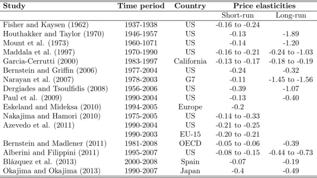
More recent studies largely vary in the estimated short- and long-run price elastic-ities. These differences are likely due to different time periods, data sets (time series vs. panel data) and econometric approaches. Okajima and Okajima (2013) and Espey and Espey (2004) give an overview of estimated short- and long-run price and income elasticities. Short- and long-run price elasticities of selected studies of residential elec-tricity demand from different geographic regions are summarized in Table 1. Price elasticities vary between -0.05 and -0.4 in the short-run, and between -0.19 and -1.89 in the long-run.
Regarding the econometric approach, most studies employ either static models or dynamic partial adjustment models. Static residential electricity demand models are usually estimated using ordinary least squares (OLS) and fixed effects (FE) or random effects (RE) models. Eskeland and Mideksa (2009) estimate a static model for residential electricity demand in 31 European countries. The main interest of the authors lies on the impact of temperature changes on electricity consumption. Also, Azevedo et al. (2011) estimate residential electricity demand using static models applied to two panels: 1990-2003 for 15 EU countries, and 1990-2004 for US states. The authors find shortrun price elasticities of 0.2 for the EU15, and 0.21 to -0.25 for the US. More recently, Cebula (2012) estimates residential electricity demand using US state-level data between 2002 and 2005. The emphasis of this study is on the key influencing factors of residential electricity consumption and the impact of state energy efficiency policies. Through a two-stage least squares approach, the author estimates that residential electricity consumption decreases with the adoption
1
A comprehensive survey of early studies on electricity demand with a focus on the residential sector is provided by Taylor (1975) and Bohi and Zimmerman (1984).
of energy efficiency programmes. Furthermore, electricity consumption decreases with price, and increases with annual cooling degree days and per capita real disposable income.
Dynamic partial adjustment models are generally more realistic than static mod-els and allow for the calculation of short- and long-run prices and income elastic-ities. Early studies by Houthakker et al. (1974) and Houthakker (1980) estimate price elasticities at the national and regional level allowing for a partial adjustment in consumption. More recently, Bernstein and Griffin (2006) and Paul et al. (2009) employ dynamic models for energy demand, although they do not address the po-tential dynamic panel bias that arises by including the lag of consumption. Both studies estimate residential electricity demand in the US. The former study uses data between 1977 and 2004, and finds short- and long-run price elasticities of -0.24 and -0.32 respectively. The latter study covers the years 1990 to 2004, and estimates short-and long-run price elasticities of -0.13 short-and -0.40 respectively. The authors claim that attempts to instrument the lag of consumption using past prices and demand did not succeed, and resulted in unstable estimates. Therefore, only least squares dummy variable (LSDV) estimates are reported. Garcia-Cerrutti (2000) estimates residential energy demand in California for the years 1983 to 1997 using dynamic random vari-ables models. The author finds a price elasticity for electricity between -0.132 and -0.172 in the short-run, and between -0.18 and -0.19 in the long-run.
Some recent studies account for dynamic panel bias and use more advanced dy-namic panel data models (e.g., panel cointegration, autoregressive distributed-lag (ARDL), generalized method of moments (GMM) estimators) or corrected FE models (e.g., Kiviet (1995) estimator). Dergiades and Tsoulfidis (2008) investigate residen-tial electricity demand in the US between 1965 and 2006 using the ARDL approach to panel cointegration. They estimate a short-run price elasticity of -0.39, and a long-run elasticity of -1.07. Bernstein and Madlener (2011) analyze residential elec-tricity demand for 18 OECD countries over the time period 1981-2008 using panel cointegration and Granger causality testing. They find a short-run price elasticity of -0.1, and a long-run elasticity of -0.39. Lower values (-0.07 and -0.19) are obtained by Blázquez et al. (2013), who apply a FE estimator and the Blundell-Bond system GMM estimator to a Spanish panel. Alberini and Filippini (2011) estimate dynamic models of residential electricity in the US and obtain slightly larger elasticities: be-tween -0.08 and -0.15 for the short-run, and bebe-tween -0.44 and -0.73 for the long-run. The Kiviet corrected FE estimator and the system Blundell-Bond GMM estimator are used to account for possible correlation between the lag of consumption and the
error term. To tackle possible endogeneity of electricity price due to measurement error, the authors also consider an instrumental variable approach.2 Finally, Kamer-schen and Porter (2004) use both a partial adjustment approach and a simultaneous equation approach. Simultaneous equation models provide negative price elasticities, whereas partial adjustment models provide positive price elasticities in some cases. The authors conclude that partial adjustment models are more appropriate in the case of energy demand estimation.
To our knowledge, none of the studies in the above literature on residential elec-tricity demand considers expectations about future prices or consumption. There are some recent studies related to gasoline price and demand: Scott (2012, 2015) include expectations about future gasoline prices do estimate gasoline demand. Anderson et al. (2013) analyze expectations about future gasoline prices and find that con-sumers typically have reasonable estimates about future gasoline prices by expecting that prices do not change from year to year. Scott (2012) estimates rational habit models for gasoline demand in the US and other countries including expectations about gas prices. One recent study in the context of residential electricity demand, Houde (2014), includes expectations about future prices in a model of residential elec-tricity demand in order to assess the success of the Energy Star programme in the US. The author assumes that consumers form time-unvarying expectations about electric-ity prices using the current local average price. The model differs from our model in that we include the lead of consumption suggested by the theoretical model used in this paper. In our empirical analysis of residential electricity demand in the US, we estimate rational habit models that include both past and lead consumption as explanatory variables in accordance with the theoretical approach proposed by Becker et al. (1994).
3
Theoretical model of residential electricity demand
In this section, we build on Becker et al. (1994) to develop a rational habit model of residential electricity consumption that extends the dynamic partial adjustment model. Households are assumed to maximize utility from energy services based on electricity (e.g. lighting, hot water, cooling, and entertainment) and other consump-tion goods. Energy services can be produced by combining two inputs: electricity and electrical appliances.
2
Another possibility to account for potential endogeneity of price is to employ simultaneous equa-tion models. However, Baltagi et al. (2002) and Baltagi (2007) find that generalized least squares (GLS), FE, and OLS estimation techniques outperform the simultaneous equation approach in most cases.
Household utility at time t is then given by:
Ut= u(St, ct), (1)
where St are energy services and ct represents all other consumption goods. Energy services are generated by the following household production function:
St= s(et, At; xt, vt), (2)
where et is electricity, At is the capital stock of electrical appliances, xt is a vector
of other (environmental) variables affecting the production of energy services, such as weather and energy substitutes, and vt is a random component that captures
uncer-tainty in the production of energy services.
Using Eqs. (1) and (2) we can write the lifetime utility function of the household as: ∞ X t=1 δt−1Ut= ∞ X t=1 δt−1u(s(et, At; xt, vt), ct), (3)
where δ = (1 + r)−1 is the constant rate of time preference and r is the interest rate. We hypothesize that the stock of electrical appliances can be adjusted over time and depends on the stock of electrical appliances in the previous period as well as the new investment in electrical appliances, It(et−1), which depends on past electricity
use. Therefore, the current stock of electrical appliances develops according to the following relationship:
At= (1 − ρ)At−1+ It(et−1), (4)
where ρ is the depreciation rate of the stock, i.e. the rate at which electrical appli-ances lose their ability to provide satisfactory energy services in the absence of energy investments. Because this stock adjustment condition relates the stock of appliances to the consumption of electricity, we can see the stock of electrical appliances as a stock of behavioural habit. Agents are habituated to a certain use of energy and appliances, which generates a stock of behavioural habit to electricity consumption. This preference can be interpreted as a status quo bias (Samuelson and Zeckhauser, 1988; Kahneman et al., 1991) that affects the depreciation rate in Eq. (4).
Using Eqs. (3) and (4) we can write the household lifetime utility maximization problem. To simplify the analysis we assume that the stock of habit fully depreciates after one period, i.e. ρ = 1, and It(et−1) = et−1 . Consequently, we get:
∞
X
t=1
s.t. e0 = E0 and ∞
X
t=1
δt−1(ct+ Ptet) = W0, (6)
where E0is the initial condition defining the level of electricity consumption in period 0, W0 is the present value of wealth, and Pt is electricity price at period t.
The first-order conditions to solve the problem above imply that the marginal utility of current electricity consumption plus the discounted marginal effect on the next period’s utility of current consumption is equal to the marginal utility of wealth multiplied by the current electricity price. Furthermore, the marginal utility of wealth equals the marginal utility of the composite good in each period. Using a quadratic utility function, the solution of the order conditions leads to the following first-difference equation:
et= θet−1+ δθet+1+ θ1Pt+ θ2xt+ δθ3xt+1+ vt. (7)
In this equation current electricity consumption is a function of past and expected future consumption, price, and all other variables, some of which are unobserved. The coefficient θ depends on the parameters of the quadratic utility function.3 Expecta-tions about environmental condiExpecta-tions, such weather or price of energy substitutes, should be captured by the coefficient of xt+1. Note that our model does not assume
that households have perfect foresight. Since expectations may be flawed, agents could be boundedly rational in their consumption decisions.
In the following empirical analysis we will investigate habits in residential elec-tricity consumption using US state-level data. Therefore, household size in the above equation (7) can actually be interpreted as state’s average household size.
4
Empirical model and data
To empirically investigate the dynamics of residential electricity consumption, we modify the first-difference equation (7) to obtain:4
eit = β0+ β1eit−1+ β2eit+1+ β3Pit+ β4P Git+ β5Yit+ β6HDDit+
+β7CDDit+ β8HSit+ β9liberal + β10T Dt+ vit, (8)
where eitis residential electricity consumption per capita in the ith state (i = 1, ..., 50)
at time t, eit−1 is the lag of electricity consumption per capita, eit+1 is the lead of 3
For further details see Baltagi and Griffin (2001). A comprehensive discussion on the interpre-tation and derivation of Eq. (7) can be found in Becker et al. (1994).
4
electricity consumption per capita5, Pit is the price of electricity, P Git is the price
of electricity substitutes (gas), Yit is income per capita, HDDit and CDDit denote,
respectively, heating degree days and cooling degree days, HSit is the housing stock,
and liberal is a dummy variable indicating if the state’s electricity market has been liberalized or not. Finally, T Dtare time-dummy variables. Note that Eq. (8) does not include expectations about environmental conditions xt+1. In a preliminary analysis we found that these covariates are collinear with the same covariates at time t and with the lag and lead of consumption. Therefore, we decided to drop them from Eq. (8) and not to use them as possible instruments. However, in our econometric approach time-invariant xt+1 as well as other unobserved time-invariant variables
are captured by fixed-effects estimators (see section 5). The residual time-variant unobserved heterogeneity is included in the disturbance term vit.
The coefficient β1 captures the impact of past consumption on current
consump-tion. Consequently, a positive and significant coefficient is consistent with the hy-pothesis that electricity consumption is a habit. Moreover, the rational habit model defined by Eq. (8) allows us to capture the behaviour of forward-looking agents.
How agents adjust their current consumption in response to expectations on fu-ture consumption sheds light on rational behaviour. The coefficient β2 measures the
impact of future consumption on current consumption. A positive coefficient would be consistent with the hypothesis of forward-looking behaviour and would support rejecting the hypothesis of myopic behaviour, which is implicit in partial adjustment models of electricity demand. From Eq. (8) we can also obtain the rate of time prefer-ence (δ) as the ratio between the estimated coefficient of eit+1 (β2) and the estimated
coefficient of eit−1 (β1).
Short- and long-run price elasticities can be obtained from Eq. (8). We can expect that electricity demand in the short run is less responsive to price changes than in the long run, as the stock of electrical appliances or behavioural habits concerning electric-ity consumption cannot be changed immediately. Some habits, such as switching off the lights when leaving a room, can be changed quickly in response to rising electricity prices. Other habits can be more persistent, for instance TV viewing time per day. Moreover, the replacement of most electrical appliances for more efficient ones repre-sents a considerable financial investment for the majority of households. Therefore, we cannot expect immediate replacement in response to changing prices, and short-run electricity consumption may depart from long-run optimal consumption. The demand
5
Although the realized values of future electricity consumption is an approximation of households’ expectations, we believe that this proxy is an acceptable indicator, assuming that deviations from the expected values are random.
does not adjust immediately to the long-run equilibrium, but gradually converges to the optimum level even when consumers are rational or boundedly rational and have expectations about future electricity demand.
Static and myopic models of electricity consumption can be derived from our rational habit model, shown in Eq. (8). In the first case, the lag and the lead variable are omitted whereas in the second case only the lead variable is excluded. In the static case, there is no delay in the adjustment process since there is no link between consumption in different periods. Static models assume that there are no costs of adjustment nor expectations that affect current decisions. The traditional dynamic partial adjustment model is more realistic as it allows for the sluggish adjustment process between optimal (long-run) consumption levels and short-run consumption. This model can be obtained from Eq. (8) assuming that agents do not take information about the future into account. Therefore, households appear to be myopic. Myopic households maximize current period utility instead of the lifetime utility function (3) under the assumption that current electricity consumption is affected by past consumption as hypothesized by Eq. (4). Finally, our full empirical model may disclose evidence of rational habits in residential electricity consumption if households take into account expectations about the future when making current consumption decisions.
An alternative to the lead consumption model (8) is to define a lead price model, which assumes that future prices represent the relevant information for rational con-sumers. This empirical approach builds on the theoretical model developed by Brown-ing (1991), who defines a demand system for many goods startBrown-ing from intertemporal nonseparability in preferences. Inspired by this work, Scott (2012, 2015) estimates lead-price rational habit models for gasoline demand based on a single equation and using a log-log functional form. Since the theoretical framework fails to derive closed-form analytical solutions, the author uses simulation to discuss the model implications. Consequently, the parameters of the suggested empirical model cannot be interpreted straightforwardly using the theoretical model. In the following empirical analysis we will focus on lead consumption models, which derive directly from our theoretical framework.6
6
Results from the estimation of a lead price model are reported in the Appendix (Table 11) and also shortly discussed in the Results section.
4.1 Data
To test the hypothesis of rational behaviour in the consumption of residential elec-tricity, we use a data set covering 51 US states (including the District of Columbia) from 1995 to 2011. For the analysis, three states (Alaska, Hawaii, and Rhode Island) are excluded because of incomplete observations. Descriptive statistics for electricity consumption and prices, and other important covariates for the remaining 48 states are presented in Table 2.
Data on residential electricity consumption (e), electricity price (P ) and gas price (P G), as well as the state of electricity market liberalization are provided by the US Energy Information Administration (EIA). The average electricity and gas prices are obtained by dividing utilities revenues by sales in the residential sector (EIA calculation). Information on income (Y ), number of inhabitants in the state (P OP ) and the number of housing units necessary to calculate average household size (HS = P OP /housing units), are from the Bureau of Economic Analysis of the US Census Bureau. Heating degree days (HDD) and cooling degree days (CDD) are obtained from the National Climatic Data Center at the National Oceanic and Atmospheric Administration (NOAA).7
The box-and-whiskers graph (Figure 1) shows the variation in residential electric-ity consumption across states over time. Residential electricelectric-ity consumption slighly increases over time. We observe that the variation within states (between variation) largely overcome the variation over time (within variation).8 The increasing trend in residential electricity consumption is associated to a decrease in price in the first half of the period. Conversely, during the second half of the period residential electricity price increased.
As we will discuss in more detail later, instrumental variables for the lead and the lag of consumption as well as for the prices are needed to estimate our model (8). For a preliminary investigation of potential instruments, Table 3 shows cross-correlations between residential electricity consumption (et), price of residential electricity and
gas (Pt and P Gt), lead electricity price (Pt+1) and spatial lag of electricity price (P−i,t), and price of gas and coal for the energy production sector (P Gpt and P Ctp).
7
Degree day is an index that reflects demand for energy to heat or cool houses. The index is obtained from daily temperature observations at major weather stations in the US. Heating (cooling) degree days are summations of negative (positive) differences between the mean daily temperature and the 65◦F base during a year.
8In the box and whiskers plot the horizontal line inside the shaded box represents the mean
consumption of residential electricity across states in each year. The width of the shaded box includes consumption in the second quartile, i.e. 50% of the states in a given year. Finally, the length of the two whiskers illustrates the third quartile of observations, i.e. 75% of the states.
Also, Figure 2 provides a graphical illustration of some price figures. The spatial lag of electricity price is calculated as the average price of bordering states for each state included in the data set. Some of these figures are clearly of interest as external instruments for the lead of consumption and electricity prices in our lead consumption models.
5
Econometric approach
For the estimation of the electricity demand equation (8), we have a balanced panel data set for 48 US states observed over the period 1995 to 2011. Therefore, the data set is characterized by a relatively long time dimension (T= 17) and a relatively small number of units (N=48). In the choice of the estimator for the dynamic model we should consider three potential econometric problems. First, due to the relatively low number of explanatory variables, a possible unobserved heterogeneity bias could be present. Second, in the consumer’s choice problem in section 3 the lifetime stream of consumption is chosen simultaneously. Therefore, we have two choice variables as explanatory variables, which implies that the lagged and lead electricity consumption could be endogenous and create the so called “dynamic panel bias” (Nickell, 1981; Roodman, 2009). This bias arises because the lagged and lead dependent variable are positively correlated with the unobserved fixed effects. Since the individual fixed effects are part of the error terms in all periods, et−1 and et+1 will be correlated
with the current error term. Third, as discussed in Alberini and Filippini (2011), the electricity price variable could suffer from a measurement error problem. This measurement error could be due to the fact that electricity price has been calculated by the US Energy Information Administration by dividing the total revenue from sales in the residential sector by total kWh sold to residential customers.
Generally, to account for unobserved time invariant heterogeneity bias using panel data, we can specify models with either fixed effects (FE) or random effects (RE). Further, to solve the endogeneity problem of some of the explanatory variables we can use a two-stage least squares (2SLS) estimator or estimators based on a the general method of moments (GMM).9 Arellano and Bond (1991), as well as Blundell and Bond (1998), propose two different estimators based on GMM. For instance, Blundell and Bond (1998) propose a system GMM estimator (GMM-BB), which uses lagged
9
Auld and Grootendorst (2004) showed that 2SLS estimators for the rational habit model using time series data may be biased when prices are endogenous and first and second lags of prices are used as instruments for the lag and lead of the dependent variable. They showed that first-differencing time series data decreases the bias. We are using FE in a panel data set which accounts for the time invariant endogeneity. To address the remaining time varying endogeneity, we use a larger battery of instruments including the spatial first and second lag and lead of the price.
first differences as instruments for equations in level as well as the lag variable in first-difference equations. However, as discussed by Baltagi et al. (2002), one possible problem of these two GMM estimators is that their properties hold for N large and small T, so the estimation results can be biased in panel data with a small number of cross-sectional units, as in our case.10 Therefore, our preferred approach to estimate the rational habits model is based on the fixed effects two-stage least squares estimator (FE2SLS). For comparison purposes, we also report the results of the FE and the GMM (in Appendix).11 Note that Baltagi and Griffin (2002) and Filippini and Masiero (2011) have successfully applied the FE2SLS estimator in dynamic demand models that include both lead and lagged values of consumption as explanatory variables. In this approach, lagged and lead values of prices, income and other covariates are used as instruments for past and future consumption. One of the advantage of the FE2SLS estimator is that it can be also used with a relatively small N.
The battery of instruments used in our estimations is quite generous. The in-struments used in the FE2SLS model are the one- and two-period lags and future values of the spatial lag of electricity price, as well as the input prices of coal and gas for the electricity sector at state level. To be a valid instrument, the variable has to be correlated with the regressors and uncorrelated with the error term. We are instrumenting three regressors: the lag of electricity consumption, the lead of electricity consumption, and the price of electricity. The price of electricity is largely determined by the generation costs of electricity. In the US, the main inputs for elec-tricity generation are coal and natural gas. In 2014, coal and natural gas accounted for 39% and 27% of total US electricity generation, respectively. The input prices for coal and gas are the main determining factors for generation costs and are determined on five regional coal and gas markets. The price differences across states should be largely due to transport and transmission costs. Therefore, the gas and coal prices at the state level should not be influenced by the level of residential electricity demand. The other major generation source, nuclear energy, accounts for around 19% of total electricity generation. However, production costs for nuclear electricity do not change considerably over time and, therefore, are not suitable as instruments.
Furthermore, we take the first and the second lag and lead of the spatial lag of electricity price as instruments. The spatial lag of electricity price represents an obvious instrument since the average of prices generated in neighbouring states is
10
For a general presentation and discussion of the estimators for dynamic panel models, see Baltagi et al. (2002).
11
In a preliminary analysis we also explored the possibility to use the corrected version of the fixed effects estimator proposed by Kiviet (1995). However, this estimator is not suitable in the presence of several endogenous variables.
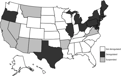
likely to be exogenous to electricity consumption within the state. The majority of US states regulated electricity markets during our study period; seven states suspended any deregulation activity (see Figure 3). For these states, prices are exogenous from neighbouring prices and should not be affected by economic shocks in neighbouring states. Only 15 states deregulated their electricity markets by 2010. Since some of these states are bordering with one or more regulated states, the spatial lag of prices is plausibly exogenous. There is a small group of deregulated states that border with deregulated states. In theory, a demand shock in one of these states affects prices in neighbouring states. However, the impact is probably negligible since electricity prices largely reflect transmission and distribution costs (35%) which are not affected by economic shocks. Therefore, to instrument both lag and lead of consumption, we use the first lag and lead of the spatial lag of electricity price (direct effect) as well as the second lag and lead of the spatial lag of electricity price (indirect effect through past and future consumption). Finally, for our GMM estimation we use the lagged values of electricity consumption and price and their first differences, the input prices of coal and gas for the electricity sector, the spatial lag of electricity price and heating degree days as well as their one- and two-period lags.
6
Estimation Results
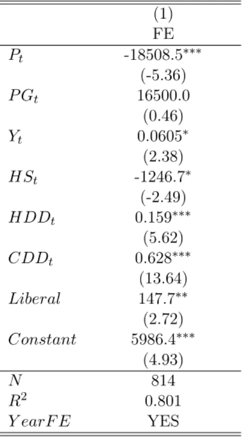
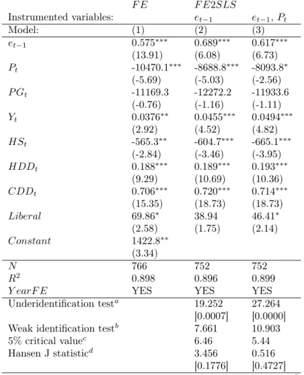
We estimate three main models: a static model, a myopic model, and the preferred lead consumption model. Results from the static and the myopic model are provided to establish a ground for comparison with the lead consumption model. Results from the static model are provided in Table 4. This model does not include lag or lead of consumption but only variables from period t. The static model shows that the price of electricity is negative and significant as expected. Results from the myopic model are reported in Table 5. Here, we only include the lag of consumption but not the lead, as the model is only backward-looking. We estimate the myopic model using fixed effects, FE2SLS instrumenting for the lag of consumption (Model 2) and instrumenting for both the lag of consumption and the current price (Model 3), and GMM. Results from the myopic model show that the price of electricity is negative and significant whereas the lag of consumption is positive and significant.
We estimate Eq. (8) using the fixed effects estimator, two FE2SLS specifications and the system GMM estimator. As previously mentioned, GMM estimators may not be suitable since we have a relatively small number of cross-sectional observations (N small), which may lead to biased results. This potential bias arises because of pos-sible serial correlation of the idiosyncratic error term in system GMM specifications.
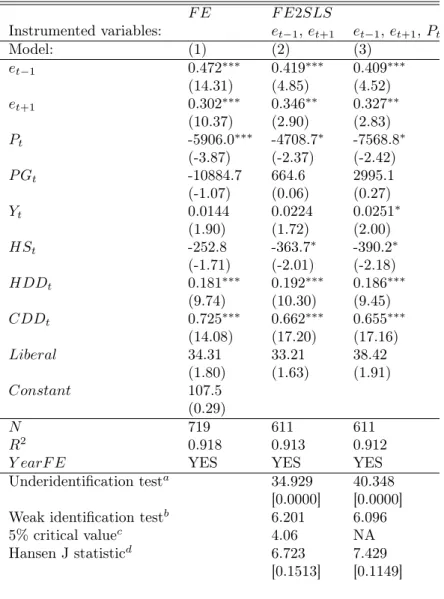
Therefore, due to the potential problems of the GMM estimator and although our results are quite robust across different specifications, the FE2SLS estimator is our preferred estimation method. To control for potential endogeneity of electricity price, we also estimate the FE2SLS model by instrumenting the price as well as the lag and lead of consumption. The estimation results of the full dynamic models of residential electricity demand are summarized in Table 6.12 For comparison purposes, we also provide the results of the GMM in the Appendix (Tables 5 and 10).
The estimated coefficients of the lag and lead of consumption have the expected positive sign and are highly significant in all estimation approaches. The values of the coefficients are fairly robust across all estimation methods, and vary between 0.409 and 0.472 for the lag and between 0.306 and 0.346 for the lead. When comparing these results with the ones from the myopic model, we can see that the lag of consumption in the myopic model is considerably larger (0.575 to 0.689) than in the lead consumption model. In the lead consumption model, the impact of the lag is smaller as part of it is captured by the lead.
The results of the lead consumption model indicate that households are taking into account both past consumption and expectations about future consumption in their current consumption decisions. This suggests that households are not myopic and seems to disagree with the specification of the traditional dynamic partial ad-justment model. Although current electricity consumption is partially driven by past consumption, there is evidence that expectations about future consumption play a role in household‘s consumption decision.
The coefficient of electricity price is negative and significant in all estimations. Income has a positive effect on current electricity consumption. The coefficient of the price of gas exhibits a negative sign in the FE and the FE2SLS estimations, although it is never significant. This might indicate that gas is not a good substitute for electricity. The main energy service produced with gas or electricity - room heating - is a long-run decision and, therefore, may not be affected by variations in current prices. The coefficients of heating and cooling degree days are highly significant and have a positive effect in all the estimations. This indicates that the use of electricity increases if there is more need to heat or cool the house. The coefficient of the electricity market liberalization dummy variable is positive and significant in the myopic model but not significant in the lead consumption model. Finally, the coefficient of the size of the household is negative and significant.
To test the validity of the FE2SLS estimation, we report several test statistics.
12
The underidentification test shows that the model is identified (we reject the null hypothesis of underidentification with a p-value of 0.0000). To exclude the possibility of weak identification, we report the Kleibergen-Papp rK Wald F statistic for weak identification, and the 5% critical value. We furthermore provide the Hansen J statistic as overidentification test for the instruments used. A rejection of the null hypothesis of joint validity would cast doubt on the validity of the instruments. The Hansen J statistic is consistent in the presence of heteroskedasticity. For both FE2SLS models we cannot reject the null hypothesis of joint validity with a p-value above 0.1. Clearly, there is still between 11% and 13% chance that we see similar results if the instruments are all exogenous or if they are all similarly endogenous.
From Eq. (8) we can obtain short- and long-run price elasticities (εt and ε∞)
of electricity demand. These are evaluated at the means of the data (e and P ) and can be calculated using the formulas derived by Becker et al. (1994). The effect on current consumption of a permanent reduction in electricity price, i.e. the short-run elasticity, is given by εt= (det/dPt)(P/e) with det/dPt= 2β3/[1−2β2+(1−4β1β2)0.5].
The long-run effect of a permanent reduction in electricity price on consumption is measured by ε∞ = (de∞/dP )(P/e) with de∞/dP = β3/(1 − β1− β2). Similarly, we
can calculate short- and long-run income elasticities using the above formulas and substituting β3 for β5 and P/e for Y /e. When consumers are not forward-looking, as
in the traditional partial adjustment model, we can use these formulas assuming that β2 is zero.
Table 7 reports the short- and long-run price elasticities calculated for all the estimation strategies including a 95% confidence interval13. Price elasticities for the myopic model range between 0.086 and 0.112 in the short run and between 0.226 and 0.298 in the long run. Short-run price elasticities in rational habit models range from 0.118 to 0.179, whereas long-run price elasticities range from 0.214 to 0.306. The calculated elasticities are fairly robust across all models and are in line with elasticities found in the literature. Overall, we can argue that residential electricity demand is relatively inelastic in the short-run. This is probably due to the cost of adjusting immediately the stock of electrical appliances in response to a change in the price or to behavioural habits in the use of electricity. Conversely, residential electricity demand is more elastic to price changes in the long run. Agents have more opportunities to adapt their behavioural habits and replace their electrical equipment. Comparing the myopic with the lead consumption model, suggests that there is no substantial difference in elasticities between the two models. This is apparently
13
surprising since the coefficients, specifically of the lag of consumption, differ between the two models. A possible reason is that we are using aggregated data. A more disaggregated, household-level dataset with higher variation in the variables may lead to different results. Note, however, that from an energy policy perspective the lack of significant differences in the estimated price elasticities does not undermine the relevant implications of our results. Indeed, the evidence of forward-looking behaviour may have policy implications. For instance, the time span between a policy approval and its implementation may take several years. This could influence the beliefs on the effectiveness of the policy measure in the near future. However, the fact that households react to the announcement before the policy is implemented may reduce this delay.
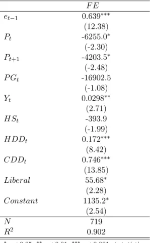
As a robustness check, we also estimate a lead price model, i.e. a model where we include the price in t + 1 to approximate expectations about future prices. We find that the coefficient of the lead of price is negative and significant, which is in line with the results from the lead consumption models (a negative impact of the lead of price equals a positive impact of the lead of consumption). Results are reported in Table 11 in the appendix.
7
Conclusions
The understanding of factors affecting residential electricity demand is of relevance to design effective energy saving policies. So far, residential electricity demand has been investigated by means of dynamic partial adjustment models. These models reflect difficulties to adjust electricity consumption over time, which may be due to bounded rationality, status quo bias or technical constraint. Our empirical analysis suggests that the traditional dynamic partial adjustment model might not be sufficient to ex-plain households’ behaviour in energy consumption. The myopic model assumes that agents do not take into account expectations about future consumption or prices when making current consumption decisions. Our empirical analysis suggests that agents need time to adjust their consumption level in response to a shock and are forward-looking when choosing electricity services to maximize intertemporal utility. However, forward-looking behavior does not assume perfect foresight. Households’ response to information about the future may be slow, biased or bounded because of mistakes in the optimization problem or the use of simple decisions rules (see Gigerenzer and Selten (2002) for a detailed classification of bounded rational behaviors).
Our analysis suggests that households adjust their consumption levels today in reaction to expected policy changes in the future. This has implications for
pol-icy implementation and evaluation. If the polpol-icy maker announces the introduction of a future policy, households may react to the announcement before the policy is implemented, i.e. households already modify today’s electricity consumption. Conse-quently, the policy design and the timing of a policy implementation should consider this anticipation effect. For instance, the policy may have immediate effects even when the implementation period is relatively long due to political and administrative constraints. Furthermore, from a research point of view, empirical methods such as difference-in-difference to evaluate the effect of energy policies, tend to neglect the anticipation effect and, therefore, underestimate their effects. In fact, the impact of a policy is generally evaluated starting at the time of policy implementation, and not at the time of its announcement. For instance, the introduction of a CO2 tax will have
a decreasing effect on energy consumption in the future but the tax already deploys part of this effect at the time of the announcement. Even though the overall effects of the tax on energy consumption do not differ significantly between the myopic and the rational habit model, the timing of these effects may differ, which could influence the policy adoption decision.
Finally, some energy policies may not affect households’ behaviour through the electricity price but rather directly through future consumption. For instance, the pol-icy maker could announce the introduction of smart metering devices or benchmarking programs where household’s energy consumption is measured against neighbours’ en-ergy consumption. The announcement of such measures could make households more aware of their levels of energy consumption and induce them to adjust their consump-tion behaviour immediately.
References
Alberini, A. and Filippini, M.: 2011, Response of residential electricity demand to price: The effect of measurement error, Energy Economics 33(5), 889–895.
Anderson, S. T., Kellogg, R. and Sallee, J. M.: 2013, What do consumers believe about future gasoline prices?, Journal of Environmental Economics and Manage-ment 66(3), 383–403.
Arellano, M. and Bond, S.: 1991, Some tests of specification for panel data: Monte carlo evidence and an application to employment equations, The Review of Eco-nomic Studies 58(2), 277–297.
Auld, M. C. and Grootendorst, P.: 2004, An empirical analysis of milk addiction, Journal of Health Economics 23(6), 1117–1133.
Azevedo, I. M. L., Morgan, M. G. and Lave, L.: 2011, Residential and regional elec-tricity consumption in the U.S. and EU: how much will higher prices reduce CO2 emissions?, The Electricity Journal 24(1), 21–29.
Baltagi, B. H.: 2007, On the use of panel data methods to estimate rational addiction models, Scottish Journal of Political Economy 54(1), 1–18.
Baltagi, B. H., Bresson, G. and Pirotte, A.: 2002, Comparison of forecast performance for homogeneous, heterogeneous and shrinkage estimators: Some empirical evidence from US electricity and natural-gas consumption, Economics Letters 76(3), 375– 382.
Baltagi, B. H. and Griffin, J.: 2001, The econometrics of rational addiction: the case of cigarettes, J Bus Econ Stat 4(19), 449–454.
Baltagi, B. H. and Griffin, J.: 2002, Rational addiction to alcohol: panel data analysis of liquor consumption, Health Economics (11), 485–491.
Becker, G. S., Grossman, M. and Murphy, K. M.: 1994, An empirical analysis of cigarette addiction, Technical report, National Bureau of Economic Research.
Becker, G. S. and Murphy, K. M.: 1988, A theory of rational addiction, The Journal of Political Economy pp. 675–700.
Bernstein, M. A. and Griffin, J. M.: 2006, Regional differences in the price-elasticity of demand for energy, National Renewable Energy Laboratory.
Bernstein, R. and Madlener, R.: 2011, Responsiveness of residential electricity demand in OECD countries: a panel cointegration and causality analysis, Technical report, E. ON Energy Research Center, Future Energy Consumer Needs and Behavior (FCN).
Blázquez, L., Boogen, N. and Filippini, M.: 2013, Residential electricity demand in Spain: New empirical evidence using aggregate data, Energy Economics 36, 648– 657.
Blundell, R. and Bond, S.: 1998, Initial conditions and moment restrictions in dynamic panel data models, Journal of Econometrics 87(1), 115–143.
Bohi, D. R. and Zimmerman, M. B.: 1984, An update on econometric studies of energy demand behavior, Annual Review of Energy 9(1), 105–154.
Browning, M.: 1991, A simple nonadditive preference structure for models of house-hold behavior over time, Journal of Political Economy pp. 607–637.
Cebula, R. J.: 2012, US residential electricity consumption: the effect of states’ pursuit of energy efficiency policies, Applied Economics Letters 19(15), 1499–1503.
Dergiades, T. and Tsoulfidis, L.: 2008, Estimating residential demand for electricity in the United States, 1965–2006, Energy Economics 30(5), 2722–2730.
Energy Information Administration, U. S.: 2010, State of electricity market restruc-turing in the U.S.
URL: http://www.eia.gov/electricity/policies/restructuring/restructure_elect.html
Eskeland, G. S. and Mideksa, T. K.: 2009, Climate change and residential electricity demand in europe, Available at SSRN: https://ssrn.com/abstract=1338835 .
Espey, J. A. and Espey, M.: 2004, Turning on the lights: A meta-analysis of residen-tial electricity demand elasticities, Journal of Agricultural and Applied Economics 36(1), 65–82.
Filippini, M. and Masiero, G.: 2011, An empirical analysis of habit and addiction to antibiotics, Empirical Economics 42(2), 471–486.
Fisher, F. M. and Kaysen, C.: 1962, The demand for electricity in the United States, Amsterdam: NorthHolland.
Garcia-Cerrutti, L. M.: 2000, Estimating elasticities of residential energy demand from panel county data using dynamic random variables models with heteroskedastic and correlated error terms, Resource and Energy Economics 22(4), 355–366.
Gigerenzer, G. and Selten, R.: 2002, Bounded rationality: The adaptive toolbox, MIT press.
Houde, S.: 2014, How consumers respond to environmental certification and the value of energy information, National Bureau of Economic Research .
Houthakker, H. S.: 1951, Some calculations on electricity consumption in Great Britain, Journal of the Royal Statistical Society. Series A (General) 114(3), 359– 371.
Houthakker, H. S.: 1980, Residential electricity revisited, The Energy Journal 1(1), 29–41.
Houthakker, H. S., Verleger, P. K. and Sheehan, D. P.: 1974, Dynamic demand anal-yses for gasoline and residential electricity, American Journal of Agricultural Eco-nomics 56(2), 412–418.
Kahneman, D., Knetsch, J. L. and Thaler, R. H.: 1991, Anomalies: The endowment effect, loss aversion, and status quo bias, The Journal of Economic Perspectives 5(1), 193–206.
Kamerschen, D. R. and Porter, D. V.: 2004, The demand for residential, industrial and total electricity, 1973–1998, Energy Economics 26(1), 87–100.
Kiviet, J. F.: 1995, On bias, inconsistency, and efficiency of various estimators in dynamic panel data models, Journal of Econometrics 68(1), 53–78.
Maddala, G. S., Trost, R. P., Li, H. and Joutz, F.: 1997, Estimation of short-run and long-run elasticities of energy demand from panel data using shrinkage estimators, Journal of Business & Economic Statistics 15(1), 90–100.
Mount, T., Chapman, L. and Tyrrell, T.: 1973, Electricity demand in the United States: an econometric analysis, Conference on energy, demand, conservation, and institutional problems, Cambridge, Massachusetts, USA.
Nakajima, T. and Hamori, S.: 2010, Change in consumer sensitivity to electricity prices in response to retail deregulation: A panel empirical analysis of the residential demand for electricity in the United States, Energy Policy 38(5), 2470–2476.
Narayan, P. K., Smyth, R. and Prasad, A.: 2007, Electricity consumption in G7 countries: A panel cointegration analysis of residential demand elasticities, Energy Policy 35(9), 4485–4494.
Nickell, S.: 1981, Biases in dynamic models with fixed effects, Econometrica 49(6), 1417.
Okajima, S. and Okajima, H.: 2013, Estimation of Japanese price elasticities of resi-dential electricity demand, 1990–2007, Energy Economics 40, 433–440.
Paul, A., Myers, E. and Palmer, K.: 2009, A partial adjustment model of US electricity demand by region, season, and sector, Resources for the Future (DP 08-50).
Roodman, D.: 2009, How to do xtabond2: An introduction to difference and system GMM in stata, Stata Journal 9(1), 86.
Samuelson, W. and Zeckhauser, R.: 1988, Status quo bias in decision making, Journal of Risk and Uncertainty 1(1), 7–59.
Scott, K. R.: 2012, Rational habits in gasoline demand, Energy Economics 34(5), 1713–1723.
Scott, K. R.: 2015, Demand and price uncertainty: rational habits in international gasoline demand, Energy 79(1), 40–49.
Taylor, L. D.: 1975, The demand for electricity: A survey, The Bell Journal of Eco-nomics 6(1), 74.
Tables and Figures
Table 1: Short- and long-run price elasticies of residential electricity demand from panel data models.
Study Time period Country Price elasticities
Short-run Long-run
Fisher and Kaysen (1962) 1937-1938 US -0.16 to -0.24
Houthakker and Taylor (1970) 1946-1957 US -0.13 -1.89
Mount et al. (1973) 1960-1071 US -0.14 -1.20
Maddala et al. (1997) 1970-1990 US -0.16 to -0.21 -0.24 to -1.03
Garcia-Cerrutti (2000) 1983-1997 California -0.13 to -0.17 -0.18 to -0.19
Bernstein and Griffin (2006) 1977-2004 US -0.24 -0.32
Narayan et al. (2007) 1978-2003 G7 -0.11 -1.45 to -1.56
Dergiades and Tsoulfidis (2008) 1956-2006 US -0.39 -1.07
Paul et al. (2009) 1990-2004 US -0.13 -0.40
Eskeland and Mideksa (2010) 1994-2005 Europe -0.2
Nakajima and Hamori (2010) 1975-2005 US -0.14 to -0.33
Azevedo et al. (2011) 1990-2004 US -0.21 to -0.25
1990-2003 EU-15 -0.20 to -0.21
Bernstein and Madlener (2011) 1981-2008 OECD -0.05 to -0.06 -0.39 Alberini and Filippini (2011) 1995-2007 US -0.08 to -0.15 -0.44 to -0.73
Blázquez et al. (2013) 2000-2008 Spain -0.07 -0.19
Okajima and Okajima (2013) 1990-2007 Japan -0.4 -0.49
Table 2: Summary statistics of main variables for the whole panel (1995-2011).
Label Variable description Mean Std. Dev. Min. Max.
e Electricity consumption per capita (in kWh) 4612.931 1229.059 2147.104 7425.204
P Electicity price (per kWh) 0.049 0.013 0.03 0.095
PG Gas price (per thousand BTU) 0.005 0.001 0.003 0.01
Y Income per capita (in US $) 15227.339 2641.341 10239.206 29294.364
HDD Heating degree days 5137.783 2012.525 555 10745
CDD Cooling degree days 1142.414 803.909 128 3870
HS Household size (POP/housing units) 2.323 0.167 1.836 2.994
POP Population/1000 5976.993 6407.277 485.16 37683.934
Table 3: Cross-correlation between price and consumption and between different price figures. Variables et Pt Pt+1 P Gt P−it P Gpt P C p t et 1.000 Pt -0.635 1.000 Pt+1 -0.619 0.981 1.000 P Gt 0.156 0.302 0.350 1.000 P−it -0.514 0.716 0.695 0.005 1.000 P Gpt 0.153 -0.042 0.038 0.569 -0.304 1.000 P Ctp 0.001 0.517 0.533 0.493 0.240 0.084 1.000
Table 4: Static model of residential electricity demand (1) FE Pt -18508.5∗∗∗ (-5.36) P Gt 16500.0 (0.46) Yt 0.0605∗ (2.38) HSt -1246.7∗ (-2.49) HDDt 0.159∗∗∗ (5.62) CDDt 0.628∗∗∗ (13.64) Liberal 147.7∗∗ (2.72) Constant 5986.4∗∗∗ (4.93) N 814 R2 0.801 Y earF E YES t statistics in parentheses ∗ p < 0.05,∗∗ p < 0.01,∗∗∗ p < 0.001
Table 5: Myopic (partial adjustment) models of residential electricity demand. F E F E2SLS Instrumented variables: et−1 et−1, Pt Model: (1) (2) (3) et−1 0.575∗∗∗ 0.689∗∗∗ 0.617∗∗∗ (13.91) (6.08) (6.73) Pt -10470.1∗∗∗ -8688.8∗∗∗ -8093.8∗ (-5.69) (-5.03) (-2.56) P Gt -11169.3 -12272.2 -11933.6 (-0.76) (-1.16) (-1.11) Yt 0.0376∗∗ 0.0455∗∗∗ 0.0494∗∗∗ (2.92) (4.52) (4.82) HSt -565.3∗∗ -604.7∗∗∗ -665.1∗∗∗ (-2.84) (-3.46) (-3.95) HDDt 0.188∗∗∗ 0.189∗∗∗ 0.193∗∗∗ (9.29) (10.69) (10.36) CDDt 0.706∗∗∗ 0.720∗∗∗ 0.714∗∗∗ (15.35) (18.73) (18.73) Liberal 69.86∗ 38.94 46.41∗ (2.58) (1.75) (2.14) Constant 1422.8∗∗ (3.34) N 766 752 752 R2 0.898 0.896 0.899
Y earF E YES YES YES
Underidentification testa 19.252 27.264
[0.0007] [0.0000]
Weak identification testb 7.661 10.903
5% critical valuec 6.46 5.44
Hansen J statisticd 3.456 0.516
[0.1776] [0.4727]
Notes: The instruments used in the F E2SLS regressions are P Gpt
(P Ctp in M odel 2), its one-period lag, and the spatial lag of electric-ity price lagged one period. First-stage regressions on the excluded instruments yield significant F-tests.
∗
p < 0.05,∗∗p < 0.01,∗∗∗p < 0.001; t statistics in round brackets p-values in square brackets;
a
Kleibergen-Papp rK LM statistic;
b
Kleibergen-Papp rk Wald F statistic;
c
Stock-Yogo weak ID test critical value (10% maximum LIML size);
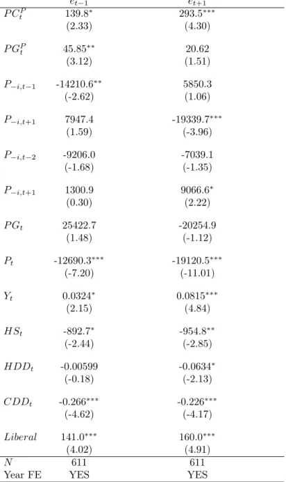
Table 6: Lead consumption model of residential electricity demand. F E F E2SLS Instrumented variables: et−1, et+1 et−1, et+1, Pt Model: (1) (2) (3) et−1 0.472∗∗∗ 0.419∗∗∗ 0.409∗∗∗ (14.31) (4.85) (4.52) et+1 0.302∗∗∗ 0.346∗∗ 0.327∗∗ (10.37) (2.90) (2.83) Pt -5906.0∗∗∗ -4708.7∗ -7568.8∗ (-3.87) (-2.37) (-2.42) P Gt -10884.7 664.6 2995.1 (-1.07) (0.06) (0.27) Yt 0.0144 0.0224 0.0251∗ (1.90) (1.72) (2.00) HSt -252.8 -363.7∗ -390.2∗ (-1.71) (-2.01) (-2.18) HDDt 0.181∗∗∗ 0.192∗∗∗ 0.186∗∗∗ (9.74) (10.30) (9.45) CDDt 0.725∗∗∗ 0.662∗∗∗ 0.655∗∗∗ (14.08) (17.20) (17.16) Liberal 34.31 33.21 38.42 (1.80) (1.63) (1.91) Constant 107.5 (0.29) N 719 611 611 R2 0.918 0.913 0.912
Y earF E YES YES YES
Underidentification testa 34.929 40.348
[0.0000] [0.0000]
Weak identification testb 6.201 6.096
5% critical valuec 4.06 NA
Hansen J statisticd 6.723 7.429
[0.1513] [0.1149]
Notes: The instruments used in the F E2SLS regression in Model (2) are the one and two-period lags and leads of the spatial lag of electricity price (P−i,t−1, P−i,t−2, P−i,t+1, P−i,t+2) and current input prices of
coal and gas for the power generation sector (P Ctp, P G p
t). In Model
(3) we also use the lagged input price of gas for the power generation sector (P Gpt−1). First stage regressions yield significant F-test. ∗
p < 0.05,∗∗p < 0.01,∗∗∗p < 0.001; t statistics in round brackets; p-values in square brackets;
a Kleibergen-Papp rK LM statistic; bKleibergen-Papp rk Wald F statistic;
c Stock-Yogo weak ID test critical value (10% maximum LIML size); d
Table 7: Short- and long-run price elasticities
Myopic model Lead consumption model
Short run
Elasticity Std. err. 95% CI Elasticity Std. err. 95% CI
FE (1) -.1118 .0196 -.1503 -.0733 -.1389 .0355 -.2084 -.0694
IV (2) -.0928 .0184 -.1289 -.0567 -.1180 .0277 -.1722 -.0637
IV price (3) -.0864 .0337 -.1526 -.0203 -.1794 .0722 -.3210 -.0379 Long run
Elasticity Std. err. 95% CI Elasticity Std. err. 95% CI
FE (1) -.2629 .0492 -.3593 -.1664 -.2795 .0771 -.4306 -.1285
IV (2) -.2982 .0705 -.4364 -.1600 -.2143 .0534 -.3190 -.1096
IV price (3) -.2256 .0860 -.3941 -.0571 -.3058 .1362 -.5728 -.0388
Figure 1: Variation in residential electricity consumption per capita across states and over time.
Figure 2: Lead and spatial-lag prices for residential electricity over time, and price of gas and coal for the production sector over time.
Figure 3: State of electricity market deregulation in the US in 2010 (Source: EIA, 2010)
Not deregulated Deregulated Suspended
Appendix
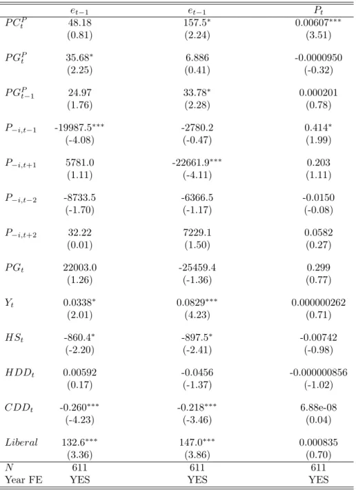
Table 8: First stage regression results of FE2SLS lead consumption model (2).
et−1 et+1 P CP t 139.8∗ 293.5∗∗∗ (2.33) (4.30) P GP t 45.85∗∗ 20.62 (3.12) (1.51) P−i,t−1 -14210.6∗∗ 5850.3 (-2.62) (1.06) P−i,t+1 7947.4 -19339.7∗∗∗ (1.59) (-3.96) P−i,t−2 -9206.0 -7039.1 (-1.68) (-1.35) P−i,t+1 1300.9 9066.6∗ (0.30) (2.22) P Gt 25422.7 -20254.9 (1.48) (-1.12) Pt -12690.3∗∗∗ -19120.5∗∗∗ (-7.20) (-11.01) Yt 0.0324∗ 0.0815∗∗∗ (2.15) (4.84) HSt -892.7∗ -954.8∗∗ (-2.44) (-2.85) HDDt -0.00599 -0.0634∗ (-0.18) (-2.13) CDDt -0.266∗∗∗ -0.226∗∗∗ (-4.62) (-4.17) Liberal 141.0∗∗∗ 160.0∗∗∗ (4.02) (4.91) N 611 611
Year FE YES YES
∗
Table 9: First stage regression results of FE2SLS lead consumption model (3). et−1 et−1 Pt P CP t 48.18 157.5∗ 0.00607∗∗∗ (0.81) (2.24) (3.51) P GP t 35.68∗ 6.886 -0.0000950 (2.25) (0.41) (-0.32) P GPt−1 24.97 33.78∗ 0.000201 (1.76) (2.28) (0.78) P−i,t−1 -19987.5∗∗∗ -2780.2 0.414∗ (-4.08) (-0.47) (1.99) P−i,t+1 5781.0 -22661.9∗∗∗ 0.203 (1.11) (-4.11) (1.11) P−i,t−2 -8733.5 -6366.5 -0.0150 (-1.70) (-1.17) (-0.08) P−i,t+2 32.22 7229.1 0.0582 (0.01) (1.50) (0.27) P Gt 22003.0 -25459.4 0.299 (1.26) (-1.36) (0.77) Yt 0.0338∗ 0.0829∗∗∗ 0.000000262 (2.01) (4.23) (0.71) HSt -860.4∗ -897.5∗ -0.00742 (-2.20) (-2.41) (-0.98) HDDt 0.00592 -0.0456 -0.000000856 (0.17) (-1.37) (-1.02) CDDt -0.260∗∗∗ -0.218∗∗∗ 6.88e-08 (-4.23) (-3.46) (0.04) Liberal 132.6∗∗∗ 147.0∗∗∗ 0.000835 (3.36) (3.86) (0.70) N 611 611 611
Year FE YES YES YES
∗
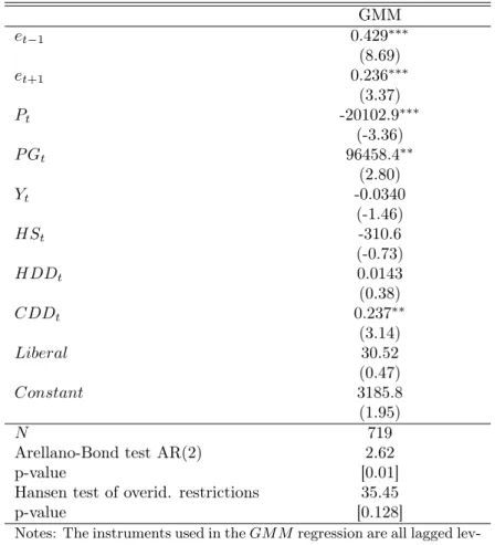
Table 10: Lead consumption model: GMM results. GMM et−1 0.429∗∗∗ (8.69) et+1 0.236∗∗∗ (3.37) Pt -20102.9∗∗∗ (-3.36) P Gt 96458.4∗∗ (2.80) Yt -0.0340 (-1.46) HSt -310.6 (-0.73) HDDt 0.0143 (0.38) CDDt 0.237∗∗ (3.14) Liberal 30.52 (0.47) Constant 3185.8 (1.95) N 719
Arellano-Bond test AR(2) 2.62
p-value [0.01]
Hansen test of overid. restrictions 35.45
p-value [0.128]
Notes: The instruments used in the GM M regression are all lagged lev-els of electricity consumption and price, P Gt, Yt, HSt, HDDt, CDDt,
Liberal, and their first differences.
∗
Table 11: Lead price model. F E et−1 0.639∗∗∗ (12.38) Pt -6255.0∗ (-2.30) Pt+1 -4203.5∗ (-2.48) P Gt -16902.5 (-1.08) Yt 0.0298∗∗ (2.71) HSt -393.9 (-1.99) HDDt 0.172∗∗∗ (8.42) CDDt 0.746∗∗∗ (13.85) Liberal 55.68∗ (2.28) Constant 1135.2∗ (2.54) N 719 R2 0.902 ∗ p < 0.05,∗∗p < 0.01,∗∗∗p < 0.001; t statistics in round brackets.